Article

Prediction of Ecosystem Service Function of Grain for Green Project Based on Ensemble Learning

1
School of Information Science & Technology, Beijing Forestry University, Beijing 100083, China
2
Research Institute of Forest Ecology, Environment and Protection, Chinese Academy of Forestry, Beijing 100091, China
3
Key Laboratory of Forest Ecology and Environment, State Forestry and Grassland Administration, Beijing 100091, China
4
Dagangshan National Key Field Observation and Research Station for Forest Ecosystem, Xinyu 338033, China
*
Author to whom correspondence should be addressed.
Forests 2021, 12(5), 537; https://doi.org/10.3390/f12050537
Submission received: 2 April 2021 / Revised: 17 April 2021 / Accepted: 23 April 2021 / Published: 26 April 2021

Abstract

:
The Grain for Green Project (GGP) was implemented over 20 years ago as one of six major forestry projects in China, and its scope of implementation is still expanding. However, it is still unclear how many ecosystem services (ESs) the project will produce in the future. The GGP’s large-scale ecological monitoring officially started in 2015 and there is a lack of early monitoring data, making it challenging to predict the future ecological benefits. Therefore, this paper proposes a method to predict future ESs by using ecological monitoring data. First, a new ensemble learning system, auto-XGBoost-ET-DT, is developed based on ensemble learning theory. Using the GGP’s known ESs in 2015, 2017, and 2019, the missing ESs of the past decade have been evaluated via reverse regression. Data from 2020 to 2022 within a convolution neural network and the coupling coordination degree model have been used to analyze the coupling between the prediction results and economic development. The results show that the growth distributions of ESs in three years were as follows: soil consolidation, 3.70–6.34%; forest nutrient retention, 2.72–3.71%; water conservation, 2.52–6.09%; carbon fixation and oxygen release, 3.00–4.64%; and dust retention, 3.82–5.75%. The coupling coordination degree of the ESs and economic development has been improved in 97% of counties in 2020 compared with 2019. The results verify a feasible ES prediction method and provide a basis for the progressive implementation of the GGP.

1. Introduction

It has been widely recognized that forests can provide ecosystem services (ESs). Much research has been produced on the quantitative evaluation of ESs, which is mainly divided into two methods: value quantity evaluation and quality evaluation. The most representative method of value quantity is the market value method proposed by Costanza [1,2]. On this basis, some researchers have put forward the equivalent factor method [3]. The method of matter quality is closer to the process of material circulation and energy exchange within an ecosystem, and the evaluation results are more favorable for ecosystem-related research. This method primarily focuses on the energy method [4] and the model method [5,6]. For the ESs of the Grain for Green Project (GGP), the model method is generally used to calculate the quality evaluation. The model method can be divided into two types: the first is a model established based on the land-use change, used to obtain the ES evaluation of GGP [7,8,9]. The GGP is mainly applied to areas with serious soil erosion and the cultivated land with a slope above 25 degrees. Therefore, its spatial distribution is very scattered. It is challenging to accurately evaluate the GGP stand with this method. The second model utilizes the assessment of ESs based on the ecological data of the GGP monitored by forest ES observation stations [10,11]. This method takes the standard age of a dominant forest species as the smallest unit to evaluate. Further, it focuses on the direct monitoring of the stand’s impact on the environment before and after the implementation of the GGP. The ecological monitoring of the GGP started as early as 2012, but the real realization of the nationwide network monitoring of forest ecosystem services through observation stations began in 2015. The monitoring network includes 32 special monitoring stations for ecological benefits, 59 forest ecological stations under CFERN, over 200 auxiliary observation points, and over 7000 sample plots. The unified ecological monitoring standard of the GGP has contributed to the accurate assessment of ESs. However, with the continuous implementation of the GGP, it is necessary to assess its future ESs in order to help the government formulate an implementation plan.
At present, some scholars have studied the simulation and prediction of ESs. However, most mathematicians carry out predictions based on land use [12,13,14]. This prediction method is not suitable for evaluating the GGP. Although the GGP causes changes in forests and farmland, not all changes are due to the GGP. The regional distribution of the GGP is very scattered, and changes within the GGP are not great compared to the changes in overall land use, making it difficult to predict the GGP’s ecological benefits. Only by using long-term positioning observation data collected in the field can accurate predictions regarding ESs be made.
The GGP has been formally implemented since 1999, and of all projects in China is the largest in scale, longest in duration, affecting the largest population, and attracting the largest amount of investment. However, since large-scale ecological monitoring for the GGP started in 2015, it has been difficult to accurately predict future ES data due to the lack of past ecological monitoring. It is important for researchers to find the most appropriate way to realize the prediction of ESs for the GGP [15].
Ensemble learning is a kind of machine learning classification. “Ensemble” refers to systems created by combining various models or classifiers [16]. Ensemble learning is generally used where there is a lack of sufficient data to correctly represent the data distribution, when various models apply to a given situation, and when the selected model cannot correctly represent the sought decision boundary [17]. In the existing research, ensemble learning is widely used in the computing [18,19,20] and medical fields [21,22]. There are few applications in the ecological field, mainly focusing on forest fire monitoring [23]. Therefore, it is feasible to use the method of ensemble learning to predict the ESs of the GGP as an innovative attempt to predict the ES of a small sample of data.
This paper uses the GGP’s quantitative ES results published in 2015, 2017, and 2019, based on long-term field positioning observation network data, and uses an integrated learning algorithm to form predictions. On this basis, a neural network is used to predict the GGP’s future ESs. The results of this study can not only fill the gaps in available ES data, but also provide a scientific basis for the further implementation of the GGP in the study area.

2. Related Work

2.1. The Prediction of Ecosystem Services

The prediction of ESs is mainly based on land-use change/cover (LUCC). Xi et al. evaluated the ESs of the Zhoushan Islands based on LUCC and simulated future changes of ESs under different scenarios [12]. Yirsaw et al. modelled and predicted ESs by evaluating future LUCC changes [13]. Gashaw et al. evaluated the impact of land-use changes on ESs in Ethiopia’s upper Blue Nile basin from 1985 to 2015 and predicted ESs in 2045 [14]. In general, the above prediction method can effectively predict ESs and simulate ESs obtained under different scenarios according to the LUCC change. However, the prediction of ESs based on LUCC is unsuitable for the GGP.

2.2. Predictions Based on Ensemble Learning

The most commonly-used ensemble learning algorithms are bagging and boosting [24]. Bagging stands for guided aggregation and is one of the earliest ensemble learning algorithms. The diversity of classifiers in bagging are obtained by resampling the training set, and the representative algorithm is a random forest algorithm. Similarly, boosting creates a set of classifiers by resampling data, and then merging them through majority voting. However, during enhancement, the resampling of boosting aims to provide the most useful training data for each successive classifier. The basic idea of boosting aims at error-prone training samples, which generate classifiers with fewer errors over the course of multiple iterations as the algorithm strengthens its learning. Representative algorithms include AdaBoost and the Gradient Boosting Decision Tree (GBDT).
In the computer field, ensemble learning is used for malicious code detection [18], abnormal detection in networks [19], and software defect prediction [20]. In the medical field, the ensemble learning method is also frequently used for disease diagnoses and predictions [21,22]. In the ecological field, the ensemble learning algorithm is sometimes used for forest fire monitoring, thus improving detection performances and reducing rates of false alarms [23]. Some researchers have also used the ensemble learning method to predict cyanobacteria blooms in the lower Han River (South Korea), improving the robustness of the model. Some scholars have improved the monitoring of soil moisture by using the ensemble learning method [25]. Ensemble learning can integrate the advantages of many different learning algorithm models at once to obtain more accurate results. It is more suitable for this study.

3. Materials and Methods

3.1. Study Area

This paper focuses on the prediction of ESs of the GGP in 14 contiguous, poverty-stricken areas in China. They are mostly distributed across the Loess Plateau, the Qinghai Tibet Plateau, some areas of the Inner Mongolia Plateau, several large desert marginal areas, and some rocky desertification areas in the South [26] (Figure 1).
The GGP’s main goal is to protect the environment, stop the cultivation of farmland with serious soil erosion, desertification and salinization, and plant trees and grasses as per local conditions to restore vegetation. The State Council arranges the State Forestry Administration, together with the National Development and Reform Commission, the Ministry of Finance, the Western Development Office of the State Council, and the State Grain Administration, to plan the project. GGP tasks are distributed to each province by the State Forestry Administration every year. A new round of the GGP has been implemented since 2014, and all farmers participating in the GGP have been given a land subsidy of 1600 yuan per mu. By 2020, the central government had invested 535.3 billion yuan in the GGP. The Chinese Government stipulates that contiguous poverty-stricken areas are key for GGP implementation, both in the present and well into the future. On the one hand, the implementation of the GGP will contribute to poverty alleviation in these regions. On the other hand, the ecological environment of these areas is poor, and the implementation of the GGP can produce more ESs, such as soil consolidation (soil consolidation reduces nitrogen loss, phosphorus loss, potassium loss, and organic matter loss), forest nutrient retention (of nitrogen, phosphorus, and potassium), water conservation, carbon fixation and oxygen release, the purification of the atmosphere (providing air negative ions, the absorption of air pollutants, dust retention, TSP retention, PM10 retention, and PM2.5 retention), forest protection (farmland protection, windbreak and sand fixation), species conservation, and so on. It is also helpful in solving the problem of soil erosion in the study area.
Forest protection is only provided by shelterbelts, and shelterbelts are not planted in all areas. Additionally, there is no accounting for the quality of species conservation. Therefore, forest protection and species conservation are not discussed in this study.

3.2. Experimental Data

In this paper, the data is provided by the GGP management centre for state forest and grassland administration, including the quantitative results of ESs and resource areas of the GGP in 2015, 2017, and 2019. Since the GGP is a forestry project, the state will assign an implementation task every year; that is, the area in which the project will be implemented. Therefore, in order to eliminate the influence of area on the accuracy of the prediction results, the mass per unit area is used for the follow-up work. The ecosystem service data of GGP can be accessed from Annex I.

3.3. Experimental Environment

The experimental environment of this study is Ubuntu 20.04 64 bit, CPU: Intel i7-10875h, GPU: titanx, RAM: 16 GB, ROM: 500 GB.
The programming language used is Python. The languages used in the framework are NumPy, Matplotlib, pandas, sklearn, and Python.

3.4. Methods

3.4.1. Ensemble Learning

The most important concept of ensemble learning is that it does not aim to generate any specific algorithm. The key point of its application is to select and fuse weak classifiers to construct strong classifiers, thereby realizing real scene prediction with a more optimized ensemble system.
In this paper, fusion training was carried out under the sklearn machine learning library developed in the Python language. SVR, linear regression, extremely randomized trees (ET), eXtreme gradient boosting (XGBoost), and the decision treeregressor (DT) were selected to analyze the data. After initial training, the R2 scores of all models were 0.74, 0.61, 0.815, 0.803, and 0.792, respectively. XGBoost, ET, and DT have the highest and most similar scores. Therefore, using these three models in tandem will result in higher prediction accuracy. Therefore, this study selected the XGBoost, ET, and DT models for integrated learning and to establish an integrated system.

3.4.2. Extremely Randomized Trees

ET is an ensemble learning method [27,28]. It is composed of multiple individual learners, and the individual learner of the ET is a decision tree [29]. A decision tree is a tree-like machine learning method which divides data samples through a series of problems or decisions until the best decision is found [30].
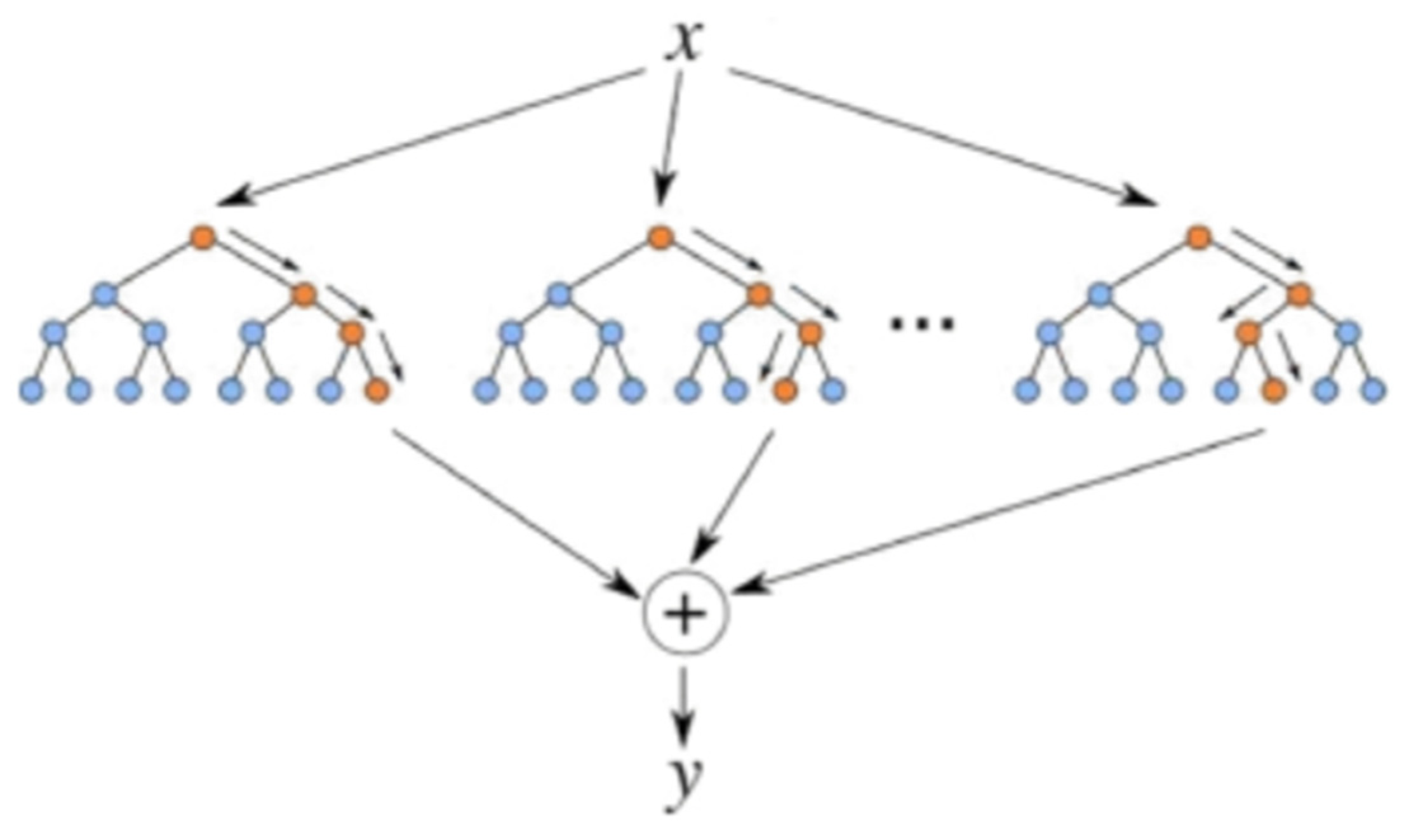
Figure 2 shows the schematic diagram of an ET algorithm. The ET algorithm uses the original training set x to sample each decision tree and uses multiple decision trees for training. As the split algorithms generated by ET are random, all the samples used are only randomly selected, and the output result is a certain average of the output of each decision tree. After the partition feature is selected, the algorithm will be more aggressive, and randomly select an eigenvalue to divide the decision tree. Therefore, the randomness of ET is reflected by the fact that the feature space of its bifurcation is randomly determined [30,31]. For this reason, an ET algorithm has better generalization than a random forest in some scenarios.

3.4.3. eXtreme Gradient Boosting

XGBoost (extreme gradient boosting) is a machine learning algorithm which originated from the GBDT model. It uses a variety of methods to accelerate its training process and improve accuracy. As a new scalable, end-to-end boosting tree algorithm, it makes accurate predictions based on tree classifiers (Figure 3), and improves operation efficiency [32,33]. It uses a prediction model based on a decision tree to work through a gradient enhancement framework [34]. It is an efficient model of reinforcement ensemble learning [35,36]. Specifically, XGBoost improves its algorithm based on a gradient lifting decision tree. The lifting tree includes a regression tree and a classification tree. The goal of the algorithm is to optimize the objective function value, which can efficiently build the lifting tree and run in parallel [37].
In addition, XGBoost has the advantage of scalability in all scenarios, and its computing speed is fast [38]. The running speed of the system on a single machine is more than ten times faster than other popular solutions, and it can be expanded to billions of examples in a distributed or memory-limited environment. It can be combined with other machine learning algorithms to obtain an algorithm with a more accurate prediction function. The scalability of XGBoost is due to several important system and algorithm optimizations. For example, a novel sparse data-sensing algorithm is used to process sparse data; a reasonable weighted quantile sketch can process data with weighted features in approximate tree learning. As parallel and distributed computing can make learning faster, the exploration of the model can be undertaken more quickly [38]. For these reasons, XGBoost is currently the best tool on the market for small-scale data [39].

3.4.4. Decision Treeregressor

Although decision treeregressor is a supervised machine learning algorithm, it is widely used in ensemble learning. An ensemble classifier is one that combines several basic classifiers together for its final classification. The classifier, for example, can be any kind of SVM or supervised DT. The DT classification model is represented by a tree structure: rather, the paths from roots to nodes represent rules. Each internal node represents a feature test, each branch represents a possible test result, each leaf node represents a classification [40], and the bifurcation path from each node represents a possible attribute value [41], mostly used for the classification of numerical and categorical data. The DT only has a single output: that is, from the root node, it can only reach one leaf node, and thus its rules are unique [42]. As a result, it can be used for data classification and prediction. Figure 4 shows a simple DT model. It includes a binary target variable y (0 or 1) and two continuous variables x1 and x2, ranging from 0 to 1. The main components of a DT model are nodes and branches, and the most important steps of establishing the model are splitting, stopping, and pruning [43].

3.4.5. Cluster Analysis

Clustering analysis performed by gathering highly similar data together, with discrete data being considered as noise in the process of experimentation. Therefore, clustering is an important part of data cleaning [44].
In a clustering problem, silhouette analysis is used to study the distance between clusters. Silhouette analysis measures the compactness of points in the same class compared with points in different classes. This measure is visualized by the silhouette graph, which provides a method to evaluate the number of classes. The silhouette value is within the range of (−1, 1), where values close to 1 indicate that the sample is far away from the adjacent class, values of 0 mean that the sample is almost on the decision boundary of two adjacent classes, and negative values mean that the sample is divided into the wrong class. Based on the silhouette analysis method, the number of the two algorithms is divided as to whether K-means (divided into 10 classes) or Birch (divided into 11 classes) is the most appropriate. The dimension reduction visualization results of clustering are shown in Figure 5 and Figure 6.
From the above figures, it can be determined that both K-means and Birch algorithms show good clustering and discretization and can eliminate some discrete data. The accuracy of the results is improved.

3.4.6. Standardization Treatment

Due to the different nature of each ecosystem service function index, each has different dimensions and orders of magnitude. When the level of each index varies greatly, if the original index value is directly used for analysis it will highlight the role of any index with a higher value in the comprehensive analysis and weaken the role of any index with a lower value. Therefore, in order to ensure the reliability of the results, it is necessary to standardize the original index data.
In this study, min/max normalization is used to normalize the data, and the original data is transformed linearly, so that the results fall to (0, 1) intervals. The conversion function is as follows:
x * = x m i n m a x m i n
where max is the maximum value of the sample data and min is the minimum value of the sample data.

3.4.7. Auto-XGBoost-ET-DT Model

We built a new model framework of ensemble learning for reverse prediction, namely an auto-XGBoost-ET-DT model. The workflow of the model is shown in Figure 7.
The basic design of the auto-XGBoost-ET-DT model is based on XGBoost, ET, and DT. First, the method in Section 3.4.4 and Section 3.4.5 was used to clean and standardize the training dataset. The processed dataset was randomly divided into three parts: 64% was used as the training set, 16% as the verification set, and 20% as the test set. The training set was used to train the above three models in the sklearn machine learning library developed by Python. Three groups of feature data were obtained. On this basis, a model fusion automaton was designed using the Python framework to determine the fusion weights for the three models. The verification set was mainly used to verify the parameters of the model in the model fusion automaton. Finally, the R2 test and mean squared error (MSE) loss function were performed using the prediction results of the test set and the auto-XGBoost-ET-DT model.
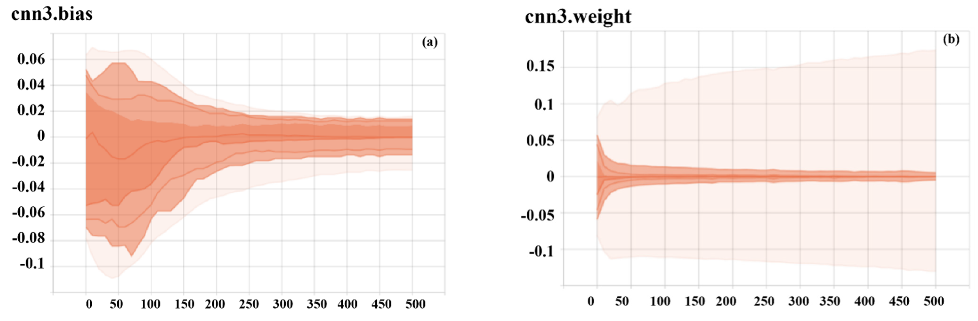
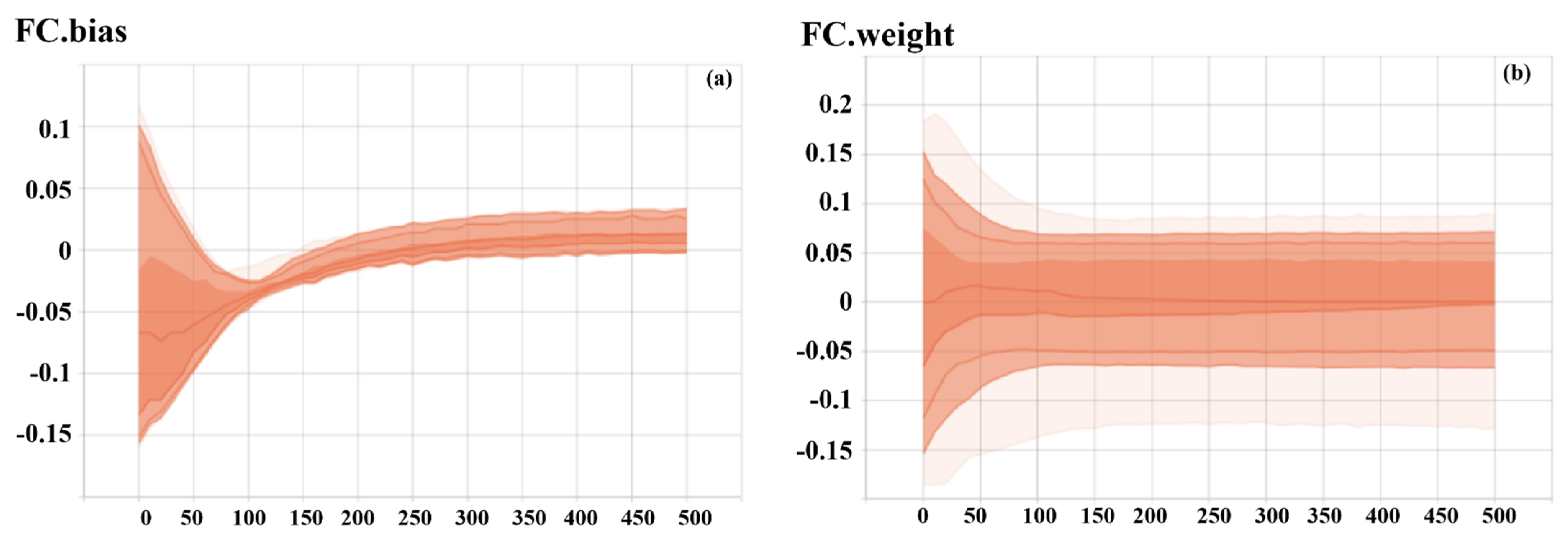
The neural network realizes the model fusion automaton. The neural network contains a fully connected layer, and only three neurons were used for weight regression. The loss function of the neural network is the mean square error (MSE). The network trains 300,000 epochs on the verification set and 1–100,000 epochs were optimized by the SGD optimization algorithm to determine the optimization direction. The Adam optimization algorithm was used to improve the optimization speed from 100,001 epochs to 200,000 epochs. The SGD optimization algorithm was used again to optimize the details from 200,001 epochs to 300,000 epochs. The basic learning rate for SGD was 1 × 10⁻², for Adam was 1 × 10⁻⁴, and for L2 was 1 × 10⁻⁴. The specific code can be found in Annex II.

3.4.8. Coupling Coordination Model

The coupling coordination model is usually used to measure the synchronous relationship between the development of the phenomenon interaction between two or more systems [45,46,47].
Considering the different dimensions between the original data of each evaluation index, the range of the standard formula was used to standardize the data. Since the indicators are all positive effects, the formula was selected as:
y i j = y i j y i j min y i j max y i j min
where i is the evaluation sample, j is the index, and yijmax and yijmin represent the maximum and minimum values of the index j in all samples, respectively.
The entropy weight method was used to calculate the weight of each index by using the difference degree of each index value. The proportion of index j in all samples Pij was as follows:
P i j = y i j + 1 j = 1 m ( y i j + 1 )
After that, we found the entropy of the index:
E i = 1 ln m j = 1 m P i j ln p i j
Finally, we calculated the entropy weight of the evaluation index:
w j = 1 E j n j = 1 n E j ,   j = 1 n w j = 1
According to the comprehensive evaluation function U = i = 1 i = m W j × y i j , we calculated the comprehensive evaluation indexes U1 and U2 of ES and ED. When 0 ≤ |U1U2| ≤ 0.1, ES and ED are synchronous. When U1U2 > 0.1, ES lags. When U1U2 < −0.1, ED lags.
The coupling correlation function is C = 2 { ( U 1 U 2 ) / [ ( U 1 + U 2 ) 2 ] } 1 2 .
In addition, the composite harmonic index needs to be calculated: T = α U 1 + β U 2 .
Where α and β represent the weights of ES and ED, respectively. Because they are equally important, α and β are both taken as 0.5. Finally, coupling coordination scheduling was calculated.
According to the coupling and cooperative scheduling, the types of coordinated development were divided into different levels, as shown in Table 1.

4. Results

4.1. Reverse Regression Based on the Auto-XGBoost-ET-DT Model

The auto-XGBoost-ET-DT model was integrated and verified by the method of 3.4.7. The model fusion automaton trained 300,000 epochs on the verification set. The training process of each model is shown in Figure 8. It shows that the weights of the three models gradually showed a smooth rising and stable trend. ET had the highest weight. The final model parameters are shown in Table 2.
The test results are shown in Figure 9. It can be seen from the figure that there was a slight fluctuation in the process of model fusion, although the R2 score rose quickly and maintained the highest common coefficient. The R2 test results showed that the auto-XGBoost-ET-DT model was accurate and true.
The integrated model processed by the model fusion automaton effectively prevented the risk of over-fitting and improved the robustness of regression. In this study, the MSELoss function was used as the criterion to evaluate the quality of the auto-XGBoost-ET-DT and determine the difference between the fusion result and the real result. The results of training the model on the training set are shown in Figure 10. The MSELoss function result was found to be close to the real value at 0.000003.
The correlation of data indicators from 2010 to 2014, 2016, and 2018 is shown in Figure 11. After a reverse regression, there was correlation among all indicators, and the correlation is generally high, between 0.41–1. In some instances, the correlation was 1, such as in the case of PM10 and PM2.5. This is mainly because PM2.5 is a kind of PM10, and generally accounts for about 70% of PM10. There was a good correlation between the indicators calculated by the reverse regression, which is consistent with the results of the correlation analysis of the initial data. The results of the regression are reliable, and can be used to predict the ESs of the GGP in the future.

4.2. Prediction of ESs of the GGP Based on Convolution Neural Network

After obtaining the ecosystem service data results of the study area from 2010 to 2019, the convolution neural network was used for prediction (Figure 12). The CNN network structure used in this study is as follows:
CNN1DNet
  • (cnn1): Conv1d(17, 32, kernel_size = (4,), stride = (1,))
  • (cnn2): Conv1d(32, 64, kernel_size = (3,), stride = (1,))
  • (pool): AdaptiveMaxPool1d(output_size = 3)
  • (relu): ReLU()
  • (cnn3): Conv1d(64, 32, kernel_size = (3,), stride = (1,))
  • (fc): Linear(in_features = 32, out_features = 17, bias = True)
  • (sigmoid): Sigmoid()
In this study, a one-dimensional CNN was used, and the parameter distribution processed by CNN is shown in Figure 13, Figure 14, Figure 15 and Figure 16. The figures demonstrate that each layer had 5000 data iterations. One-dimensional CNN can be regarded as a linear regression equation. When there is a significant linear correlation between variables X and y, the linear equation y = ax + b of the optimal line is determined by the principle of the least square method. The distance between the ideal regression point and any straight line is smaller than that of any other straight line. The regression intercept b of each layer represents the intercept of the line on the y axis and the starting point of the line. The regression coefficient a represents the slope of the straight line. Its practical significance is to explain the number of changes in the average y when x changes by one unit. In other words, y changes by a units for every 1 unit increase.
In the first layer, the CNN used Gaussian distribution to initialize the processed data distribution, which converged gradually from the initial discrete state (Figure 13). Therefore, the data were increasingly in line with recent expectations.
The second layer used the rectified linear activation function (ReLU) to increase the nonlinearity of the neural network model, and introduced nonlinear factors to the neurons. The neural network can arbitrarily approximate any nonlinear function, and therefore the neural network can be applied to many nonlinear models. It can be seen in Figure 14 that almost all intercept terms were greater than 0 in the later stage, which is due to the generation of the GGP data. The service data provided by the state system had no negative number, thus almost all intercept terms converged to greater than 0 in the second layer of the CNN, and the weight was more convergent than that in the first layer.
In the third layer of the CNN, both the intercept term and the weight achieved their final convergence. However, fluctuations can be seen from Figure 15, especially in Figure 15a, due to the fluctuations of intercept and weight between the local optimal solution and global optimal solution in the third layer CNN. However, the global optimal solution was finally achieved.
A sigmoid function was used to process the final FCN layer so that the final output was positive, and the data interval was (0,1); this makes the final results easier to regress, and the prediction model can achieve better results. In Figure 16a, the intercept term converged upward in the last iteration, which is due to the fact that the final results predicted by the model were close to 0.5 after the data was standardized. Additionally, Figure 15b and Figure 16b show that the weights in the FCN layer were more dispersed than those in the third layer CNN. This is mainly because the number of neurons in the FCN layer was reduced to converge into one unit to realize the output of the final prediction data. At this time, a large number of models were not required to predict the data, and so the weight distribution was more dispersed.
According to the gap between the prediction result of loss function and label data, a loss convergence chart is generated (Figure 17). In this case, the MSE loss function represents the degree to which the current CNN did not fit the training data. The loss value continues decreasing in Figure 17. Although the loss value rose after finding the optimal solution, the range of recovery was not large. In general, the CNN used in this prediction is representative and close to the correct prediction result, indicating the reliability of the prediction result.

4.3. Comparison of Long Short-Term Memory Network Prediction

In the comparative study, because deep neural networks (DNNs) cannot accurately predict the sample data with time series information, a long short-term memory neural network (LSTM) was selected. This was used to predict the ecosystem service function of the project, and its results were compared with the CNN for both the MSELoss function and R2 test. The results are shown in Figure 18. The LSTM was trained based on the MSELoss function, and the result of MSELoss function cannot be regressed (Figure 18a). In contrast, the convergence effect of the CNN’s MSELoss function was excellent. In Figure 18b, the initial value of LSTM was below −8000. After epoch iteration, although it was improved, its limit value only reached about −2000, which is far from the regression value of the sample. Comparatively, the CNN performed well using the R2 test, with an R2 score of 96.3%, which is very close to the real value.

4.4. Prediction Results of ESs of the GGP

Due to outlier data, dirty data, and empty data being eliminated during pre-test data cleaning, the final result looks at only 660 counties. As calculated by the prediction model, the data of the GGP ecosystem service quality from 2020 to 2022 are shown in Table 3. It should be noted that this prediction does not consider the increase of the GGP’s vegetation restoration resource area, and takes the vegetation restoration resource area in 2019 as the criterion.

5. Discussion

5.1. Analysis of ESs of the GGP

The results show that the ecosystem service function will continue to increase with the continued implementation of the GGP. The increases of the ecosystem service functions in three years are 3.70–6.34% for soil consolidation, 2.72–3.71% for forest nutrient retention, 2.52–6.09% for water conservation, 3.00–4.64% for carbon fixation and oxygen release, and 3.82–5.75% for dust retention. The biggest annual increase is in the function of soil conservation, and the biggest difference in annual increases regards the function of water conservation, which is particularly important when considering that soil and water conservation are the GGP’s primary goals. When the project task is assigned each year, the GGP is mainly considered for areas with serious soil erosion. After the implementation of the project in a given area, the degree of soil erosion is reduced, and the functions of soil conservation and water conservation play a greater role.

5.2. Comparison with Other Predictions

Lin et al. evaluated the Qingjiang River Basin and predicted ESs in the next 20 years based on land-use changes and ecological disasters [48]. Lin’s research is located in the Wuling mountain area, meaning that their research results have certain comparability. According to Lin’s research results, the annual increase of ESs in the Qingjiang River Basin from 2020 to 2035 is about 1.68–5.88%, similar to our research results (2.52–6.34%). Our research results are high because we only considered the implementation of the GGP, while Lin considered the negative impact of ecological disasters.
When Yirsaw used land-use to predict ES [13], the relative errors of all LUCC classes were less than 5%. In our study, the R2 test of the data in the first 10 years based on the auto-xgboost-et-DT model reverse prediction showed that the score almost approached 0, proving that the accuracy was more than 99.9%.
Biomass carbon increased by 8% from 2001 to 2050 under the forest incentives policy scenario in Lawler’s research on the prediction of ESs in the United States based on land-use changes. The GGP is also a kind of forest-incentive policy. Our prediction of carbon growth is between 4.87% and 6.39% per year, larger than in Lawler’s study. This is mainly due to the fact that our carbon growth considers biomass carbon and soil carbon. Additionally, most GGP stands are in the stage of vigorous growth, providing much more carbon sequestration than mature or overly mature stands. The time scale predicted by Lawler is larger. On the one hand, the accuracy of the prediction results may be reduced. On the other hand, the carbon sequestration function will be reduced when the trees are almost mature in 50 years.
It is not a challenge to determine from the above comparison that our research has some limitations, since the time sequence of the training data used in the prediction was too short thus the prediction accuracy of the ESs was reduced. Simultaneously, compared with the prediction based on LUCC, we cannot simulate the changes of ESs under different scenarios. These problems need to be further explored in the future.
However, our method has some advantages in prediction accuracy. Further, the prediction based on the ensemble learning method is more suitable for the prediction of the GGP ESs. It can also realize the prediction of multiple ESs at the same time instead of only obtaining a total value of the ESs. This prediction has higher ecological significance.

5.3. Coordination Types of ES and Economic Development of the GGP

The types of coordinated development of ecological and economic benefits of the GGP in 2017, 2019 and 2020 are compared and analysed, as shown in Figure 19. In the study area, the development degree of ecological and economic benefits has changed significantly. In 2017, 65% of the counties achieved the synchronous development of ecological economy, while 17% of the counties have fallen behind in ecology, especially in the central region, where the ecological environment particularly needs to be improved. At the same time, economic development is relatively low in the western and eastern regions, and their ecological footprints need to be further optimized. By 2019, most of the counties are lagging in ecological development, accounting for 92%. Only 3% of the counties have achieved the same level of development in both ecology and economy. The counties in the central region, which used to be ahead in terms of ecological development, have also switched into a development mode focused more on the economy. In 2020, most of the counties are in a state of prioritizing ecological development, while their economic development lags, accounting for 84%. Only 9% of the counties have coordinated their development of ecology and economy, and the remaining 7% are in a state of prioritizing economic development.
The main reason for the difference in ecological and economic development between 2017 and 2019 is that 2020 is an important point in time for China’s anti-poverty efforts. The state has made great efforts to help poorer areas grow economically, and the economy was strongly prioritized in 2019. By 2020, ecological development will be significantly ahead, as the GGP will develop more than the economy within this year.

5.4. Coupling Analysis of ESs and Economic Development of the GGP

The maps below show the distribution and degree of coupling coordination within the study area (Figure 20a–c), demonstrating that the coupling coordination degree of ESs and economic benefits of the GGP have a high degree of coordination. Most regions have achieved extreme coordination and coupling, accounting for 90%. The coupling coordination degree of 97% of counties has been improved compared with that of 2019 (Figure 20d), which is 10% higher than that of 2017. This not only shows that the ESs and economic development of the GGP in the concentrated contiguous destitute areas have proceeded at largely the same pace for two years, but also that the concentrated contiguous destitute areas are at a high level of ecosystem service improvement and economic development coordination, with high consistency and mutual influence. At the same time, at present, when the ecosystem service function of the GGP is improved, the concentrated contiguous destitute areas achieve a high level of economic benefits. This proves that “green water and green mountains” is a necessary developmental underpinning for “golden water and silver mountains”. In addition, the degree of coupling coordination is no longer distributed along the “Hu Huanyong line,” but instead is more dispersed. With the improvement of ecological benefits, the development of some regions will break the existing concept of dividing the two sides of China’s economic development along the “Hu Huanyong line”.

6. Conclusions

Using an ensemble learning algorithm to predict the quality of the GGP ESs, results were obtained which show that with the continued implementation of the GGP, ESs will also continue to increase. This plays an important role in the protection of China’s ecological environment and achieves the implementation goal of the project.
The coupling coordination analysis of ESs and the economic development of the GGP shows that 97% of the counties in the study area are in a state of extreme coupling, which is 10% higher than that of 2017 and 84% higher than that of 2019. The experimental results effectively confirm that at present, when the ESs of the GGP are improved, the economic benefits of contiguous destitute areas can achieve greater development space. The implementation of the GGP needs to be further promoted. At the same time, it is important for continuing economic development to manage and protect existing GGP resources to the maximum extent and continue to improve ecosystem service functions. Finally, the implementation of the project has made a certain contribution to the realization of the goal of poverty alleviation in China.
The time-series data of the ESs of the GGP effectively increased using the research method proposed in this paper. The ESs that the GGP can produce in the future are successfully predicted. This provides a reliable scientific basis for the further implementation of the GGP. It also provides a new method for ES prediction. As time goes on, the GGP will evaluate ESs over a longer time period, greatly improving the prediction accuracy of the ESs. Further, the GGP is greatly influenced by various policies published by the state. Future research should capture the focus, emotion, and value tendency of the Grain for Green Projects based on big data technology and integrate the prediction of emotional tendency and attitudes to better realize the ESs of the GGP.

Author Contributions

Conceptualization, methodology, writing—review and editing, funding acquisition, project administration, B.W. and X.N.; validation, H.L. and X.N.; formal analysis, data curation, writing—original draft preparation, H.L.; All authors have read and agreed to the published version of the manuscript.

Funding

This research was funded by the Fundamental Research Funds for the Central Non-profit Research Institution of CAF (CAFYBB2020ZD002, CAFYBB2020ZE003), the Ecological benefit monitoring of The Grain for Green Project, Forest resources accounting and Forestry Green Development in China.

Institutional Review Board Statement

Not applicable.

Informed Consent Statement

Not applicable.

Data Availability Statement

In this paper, the socio-economic data is taken from the National Bureau of statistics and the “CEInet Statistics Database” at https://db.cei.cn/, accessed on 18 April 2021 (In Chinese).

Acknowledgments

The ecosystem service data of the GGP is provided by the State Forestry and grassland administration. We gratefully acknowledge their invaluable cooperation in this work.

Conflicts of Interest

The authors declare no conflict of interest.

References

  1. Costanza, R.; d’Arge, R.; De Groot, R.; Farber, S.; Grasso, M.; Hannon, B.; Limburg, K.; Naeem, S.; O’Neill, R.V.; Paruelo, J.; et al. The value of the world’s ecosystem services and natural capital. Nature 1997, 387, 253–260. [Google Scholar] [CrossRef]
  2. Costanza, R.; Kubiszewski, I.; Ervin, D.; Bluffstone, R.; Boyd, J.; Brown, D.; Chang, H.; Dujon, V.; Granek, E.; Polasky, S.; et al. Valuing Ecological Systems and Services. F1000 Biol. Rep. 2011, 3, 14. [Google Scholar] [CrossRef] [Green Version]
  3. Odum, H.T.; Odum, E.P. The Energetic Basis for Valuation of Ecosystem Services. Ecosystems 2000, 3, 21–23. [Google Scholar] [CrossRef]
  4. Bagstad, K.J.; Villa, F.; Batker, D.; Harrison-Cox, J.; Voigt, B.; Johnson, G.W. From theoretical to actual ecosystem services: Mapping beneficiaries and spatial flows in ecosystem service assessments. Ecol. Soc. 2014, 19, 706–708. [Google Scholar] [CrossRef] [Green Version]
  5. Sharps, K.; Masante, D.; Thomas, A.R.C.; Jackson, B.M.; Cosby, B.J.; Emmett, B.A. Comparing strengths and weaknesses of three ecosystem services modelling tools in a diverse uk river catchment. Sci. Total. Environ. 2017, 584–585, 118–130. [Google Scholar] [CrossRef] [PubMed] [Green Version]
  6. Boumans, R.; Roman, J.; Altman, I.; Kaufman, L. The Multiscale Integrated Model of Ecosystem Services (MIMES): Simulating the interactions of coupled human and natural systems. Ecosyst. Serv. 2015, 12, 30–41. [Google Scholar] [CrossRef]
  7. Dang, D.; Li, X.; Li, S.; Dou, H. Ecosystem Services and Their Relationships in the Grain-for-Green Programme—A Case Study of Duolun County in Inner Mongolia, China. Sustainability 2018, 10, 4036. [Google Scholar] [CrossRef] [Green Version]
  8. Yu, Q.; Feng, C.-C.; Xu, N.; Guo, L.; Wang, D. Quantifying the Impact of Grain for Green Program on Ecosystem Service Management: A Case Study of Exibei Region, China. Int. J. Environ. Res. Public Health 2019, 16, 2311. [Google Scholar] [CrossRef] [Green Version]
  9. Wang, H.; Liu, G.; Li, Z.; Ye, X.; Fu, B.; Lü, Y. Analysis of the Driving Forces in Vegetation Variation in the Grain for Green Program Region, China. Sustainability 2017, 9, 1853. [Google Scholar] [CrossRef] [Green Version]
  10. Wang, B.; Gao, P.; Niu, X.; Sun, J. Policy-driven China’s Grain to Green Program: Implications for ecosystem services. Ecosyst. Serv. 2017, 27, 38–47. [Google Scholar] [CrossRef]
  11. Wei, W.; Wang, B.; Niu, X. Soil Erosion Reduction by Grain for Green Project in Desertification Areas of Northern China. Forests 2020, 11, 473. [Google Scholar] [CrossRef]
  12. Xi, H.; Cui, W.; Cai, L.; Chen, M.; Xu, C. Evaluation and Prediction of Ecosystem Service Value in the Zhoushan Islands Based on LUCC. Sustainability 2021, 13, 2302. [Google Scholar] [CrossRef]
  13. Yirsaw, E.; Wu, W.; Shi, X.; Temesgen, H.; Bekele, B. Land Use/Land Cover Change Modeling and the Prediction of Subsequent Changes in Ecosystem Service Values in a Coastal Area of China, the Su-Xi-Chang Region. Sustainability 2017, 9, 1204. [Google Scholar] [CrossRef] [Green Version]
  14. Gashaw, T.; Tulu, T.; Argaw, M.; Worqlul, A.W.; Tolessa, T.; Kindu, M. Estimating the impacts of land use/land cover changes on Ecosystem Service Values: The case of the Andassa watershed in the Upper Blue Nile basin of Ethiopia. Ecosyst. Serv. 2018, 31, 219–228. [Google Scholar] [CrossRef]
  15. Song, X.; Peng, C.; Zhou, G.; Jiang, H.; Wang, W. Chinese Grain for Green Program led to highly increased soil organic carbon levels: A meta-analysis. Sci. Rep. 2014, 4, 1–7. [Google Scholar] [CrossRef] [PubMed] [Green Version]
  16. Polikar, R. Ensemble Learning. Scholarpedia 2009, 4, 2776. [Google Scholar] [CrossRef]
  17. Dietterich, T.G. Ensemble Methods in Machine Learning. Int. Workshop Mult. Classif. Syst. 2000, 1857, 1–15. [Google Scholar]
  18. Xue, D.; Li, J.; Wu, W.; Tian, Q.; Wang, J. Homology analysis of malware based on ensemble learning and multifeatures. PLoS ONE 2019, 14, e0211373. [Google Scholar] [CrossRef]
  19. Sornsuwit, P.; Jaiyen, S. Intrusion detection model based on ensemble learning for U2R and R2L attacks. In Proceedings of the 2015 7th International Conference on Information Technology and Electrical Engineering (ICITEE), Chiang Mai, Thailand, 29–30 October 2015; pp. 354–359. [Google Scholar]
  20. Li, R.; Zhou, L.; Zhang, S.; Liu, H.; Huang, X.; Sun, Z. Software defect prediction based on ensemble learning. In Proceedings of the 2019 2nd International Conference on Data Science and Information Technology, Seoul, Korea, 19–21 July 2019; pp. 1–6. [Google Scholar] [CrossRef] [Green Version]
  21. Fitriyani, N.L.; Syafrudin, M.; Alfian, G.; Rhee, J. Development of Disease Prediction Model Based on Ensemble Learning Approach for Diabetes and Hypertension. IEEE Access 2019, 7, 144777–144789. [Google Scholar] [CrossRef]
  22. Lo, Y.T.; Fujita, H.; Pai, T.W. Prediction of coronary artery disease based on ensemble learning approaches and co-expressed observations. J. Mech. Med. Biol. 2016, 16, 1640010. [Google Scholar] [CrossRef]
  23. Xu, R.; Lin, H.; Lu, K.; Cao, L.; Liu, Y. A Forest Fire Detection System Based on Ensemble Learning. Forests 2021, 12, 217. [Google Scholar] [CrossRef]
  24. Nguyen, K.A.; Chen, W.; Lin, B.-S.; Seeboonruang, U. Comparison of Ensemble Machine Learning Methods for Soil Erosion Pin Measurements. ISPRS Int. J. Geo-Inf. 2021, 10, 42. [Google Scholar] [CrossRef]
  25. Shin, J.; Yoon, S.; Cha, Y. Prediction of cyanobacteria blooms in the lower Han River (South Korea) using ensemble learning algorithms. Desalin. Water Treat. 2017, 84, 31–39. [Google Scholar] [CrossRef] [Green Version]
  26. Ge, Y.; Yuan, Y.; Hu, S.; Ren, Z.; Wang, X.; Wu, Y. Space–time variability analysis of poverty alleviation performance in China’s poverty-stricken areas. Spat. Stat. 2017, 21, 460–474. [Google Scholar] [CrossRef]
  27. Geurts, P.; Erns, T.D.; Wehenkel, L. Extremely randomized trees. Mach. Learn. 2006, 63, 3–42. [Google Scholar] [CrossRef] [Green Version]
  28. Louppe, G. Understanding random forests: From theory to practice. Cornell Univ. Libr. 2014, 10. [Google Scholar] [CrossRef]
  29. Tyralis, H.; Papacharalampous, G.; Langousis, A. Super ensemble learning for daily streamflow forecasting: Large-scale demonstration and comparison with multiple machine learning algorithms. Neural Comput. Appl. 2020, 33, 3053–3068. [Google Scholar] [CrossRef]
  30. Murthy, S.K. Automatic construction of decision trees from data: A multi-disciplinary survey. Data Min. Knowl. Discov. 1998, 2, 345–389. [Google Scholar] [CrossRef]
  31. Mehta, P.; Bukov, M.; Wang, C.H.; Day, A.G.; Richardson, C.; Fisher, C.K.; Schwab, D.J. A high-bias, low-variance introduction to machine learning for physicists. Phys. Rep. 2019, 810, 1–124. [Google Scholar] [CrossRef]
  32. Wang, F.; Ross, C.L. Machine learning travel mode choices: Comparing the performance of an extreme gradient boosting model with a multinomial logit model. Transp. Res. Rec. 2018, 2672, 35–45. [Google Scholar] [CrossRef] [Green Version]
  33. Hsu, C.N.; Liu, C.L.; Tain, Y.L.; Kuo, C.Y.; Lin, Y.C. Machine Learning Model for Risk Prediction of Community- Acquired Acute Kidney Injury Hospitalization from Electronic Health Records: Development and Validation Study. J. Med. Internet. Res. 2020, 22, e16903. [Google Scholar] [CrossRef]
  34. Chen, Z.; Jiang, F.; Cheng, Y.; Gu, X.; Liu, W.; Peng, J. Xgboost classifier for ddos attack detection and analysis in sdn-based cloud. In Proceedings of the 2018 IEEE International Conference on Big Data and Smart Computing (BigComp), Shanghai, China, 15–17 January 2018; pp. 251–256. [Google Scholar]
  35. Friedman, J.; Hastie, T.; Tibshirani, R. Additive logistic regression: A statistical view of boosting (with discussion and a rejoinder by the authors). Ann. Stat. 2000, 28, 337–407. [Google Scholar] [CrossRef]
  36. Friedman, J.H. Greedy Function Approximation: A Gradient Boosting Machine. Ann. Stat. 2001, 29, 1189–1232. [Google Scholar] [CrossRef]
  37. Zheng, H.; Yuan, J.; Chen, L. Short-term load forecasting using EMD-LSTM neural networks with a Xgboost algorithm for feature importance evaluation. Energies 2017, 10, 1168. [Google Scholar] [CrossRef] [Green Version]
  38. Chen, T.; Guestrin, C. Xgboost: A scalable tree boosting system. In Proceedings of the 22nd ACM Sigkdd International Conference on Knowledge Discovery and Data Mining, San Francisco, CA, USA, 13–17 August 2016; pp. 785–794. [Google Scholar] [CrossRef] [Green Version]
  39. Morde, V. Xgboost algorithm: Long may she reign. Towards Data Sci. 2019. Available online: https://towardsdatascience.com/https-medium-com-vishalmorde-xgboost-algorithm-long-she-may-rein-edd9f99be63d (accessed on 20 August 2019).
  40. Pal, M. Ensemble learning with decision tree for remote sensing classification. World Acad. Sci. Eng. Technol. 2007, 36, 258–260. [Google Scholar]
  41. Bhukya, D.P.; Ramachandram, S. Decision tree induction: An approach for data classification using AVL-tree. Int. J. Comput. Electr. Eng. 2010, 2, 660. [Google Scholar] [CrossRef] [Green Version]
  42. Kanev, A.; Nasteka, A.; Bessonova, C.; Nevmerzhitsky, D.; Silaev, A.; Efremov, A.; Nikiforova, K. Anomaly detection in wireless sensor network of the “smart home” system. In Proceedings of the 2017 20th Conference of Open Innovations Association (FRUCT), St. Petersburg, Russia, 3–7 April 2017; pp. 118–124. [Google Scholar]
  43. Song, Y.Y.; Ying, L.U. Decision tree methods: Applications for classification and prediction. Shanghai Arch. Psychiatry 2015, 27, 130. [Google Scholar] [PubMed]
  44. Rahul, K.; Banyal, R.K.; Goswami, P. Analysis and processing aspects of data in big data applications. J. Discret. Math. Sci. Cryptogr. 2020, 23, 385–393. [Google Scholar] [CrossRef]
  45. Zhang, X.; Xu, Z. Functional Coupling Degree and Human Activity Intensity of Production–Living–Ecological Space in Underdeveloped Regions in China: Case Study of Guizhou Province. Land 2021, 10, 56. [Google Scholar] [CrossRef]
  46. Ariken, M.; Zhang, F.; Liu, K.; Fang, C.; Kung, H.T. Coupling coordination analysis of urbanization and eco-environment in Yanqi Basin based on multi-source remote sensing data. Ecol. Indic. 2020, 114, 106331. [Google Scholar] [CrossRef]
  47. Shi, T.; Yang, S.; Zhang, W.; Zhou, Q. Coupling coordination degree measurement and spatiotemporal heterogeneity between economic development and ecological environment—Empirical evidence from tropical and subtropical regions of China. J. Clean. Prod. 2020, 244, 118739. [Google Scholar] [CrossRef]
  48. Lin, Z.; Ye, X.; Wei, Q.; Xin, F.; Lu, Z.; Kudva, S.; Dai, Q. Ecosystem Services Value Assessment and Uneven Development of the Qingjiang River Basin in China. Sustainability 2017, 9, 2356. [Google Scholar] [CrossRef] [Green Version]
Figure 1. Study location: contiguous poverty-stricken regions in China.
Forests 12 00537 g001
Figure 2. Schematic diagram of ET.
Forests 12 00537 g002
Figure 3. Flow chart of XGBoost.
Forests 12 00537 g003
Figure 4. DT model process.
Forests 12 00537 g004
Figure 5. Dimensionality reduction visualization of PCA (a), tSNE-PCA (b), and tSNE-Random (c) under K-Means.
Forests 12 00537 g005
Figure 6. Dimensionality reduction visualization of PCA (a), tSNE-PCA (b), and tSNE-Random (c) under Birch.
Forests 12 00537 g006aForests 12 00537 g006b
Figure 7. Workflow of the auto-XGBoost-ET-DT.
Forests 12 00537 g007
Figure 8. Single model weight.
Forests 12 00537 g008
Figure 9. R2 test of the auto-XGBoost-ET-DT.
Forests 12 00537 g009
Figure 10. Convergence trend based on MSELoss.
Forests 12 00537 g010
Figure 11. Thermodynamic diagram of correlation between indexes after reverse regression. From (ag) the thermal relationship diagrams between data from 2010, 2011, 2012, 2013, 2014, 2016, and 2018 are shown. a: soil consolidation; b: reduce nitrogen loss; c: reduce phosphorus loss; d: reduce potassium loss; e: reduce organic matter loss; f: forest nutrient retention of nitrogen; g: forest nutrient retention of phosphorus; h: forest nutrient retention of potassium; i: water conservation; j: carbon fixation; k: oxygen release; l: provision of air negative ions; m: absorption of air pollutants; n: dust retention; o: TSP; p: PM10; q: PM2.5.
Forests 12 00537 g011
Figure 12. Convolution neural network algorithm flow.
Forests 12 00537 g012
Figure 13. Distribution of the (a) intercept and (b) weight of the first layer CNN.
Forests 12 00537 g013
Figure 14. Distribution of the (a) intercept and (b) weight of the second layer CNN.
Forests 12 00537 g014
Figure 15. Distribution of the (a) intercept and (b) weight of the third layer CNN.
Forests 12 00537 g015
Figure 16. Distribution of the (a) intercept and (b) weight of the FCN.
Forests 12 00537 g016
Figure 17. Convergence diagram of MSELoss.
Forests 12 00537 g017
Figure 18. Comparison of the (a) MSELoss and (b) R2 test between the CNN and LSTM.
Forests 12 00537 g018
Figure 19. Subtraction of the comprehensive evaluation index between ecosystem services and economic development in (a) 2017, (b) 2019, and (c) 2020.
Forests 12 00537 g019
Figure 20. Coupling coordination between ESs and economic development in 2017 (a), 2019 (b), and 2020 (c), and changes in 2019 and 2020 (d).
Forests 12 00537 g020
Table 1. Classification of coordination coupling.
Coordination CouplingEvaluation Grade
0~0.29low coordination coupling
0.3~0.49moderate coordination coupling
0.5~0.79high coordination coupling
0.8~1extreme coordination coupling
Table 2. Parameters of the auto-XGBoost-ET-DT.
ModelParameter
XGBoost0.299830
ET0.671922
DT0.108755
Table 3. Prediction results based on the CNN.
YearSoil Consolidation (×104 t/a)Forest Nutrient Retention (×104 t/a)Water Conservation
(×108 m3/a)
Carbon Fixation and Oxygen Release (×104 t/a)Dust Retention (×104 t/a)
202033,402.4147.44211.048847.8525,040.31
202134,937.7548.73216.359113.4225,997.28
202236,834.1850.54229.529536.3927,490.83
Publisher’s Note: MDPI stays neutral with regard to jurisdictional claims in published maps and institutional affiliations.

