Article

What Factors Shape Spatial Distribution of Biomass in Riparian Forests? Insights from a LiDAR Survey over a Large Area

1
TERRA Teaching and Research Centre (Forest Is Life), Gembloux Agro-Bio Tech, University of Liege, Passage des Déportés 2, 5030 Gembloux, Belgium
2
University Rennes 2, CNRS UMR LETG, Place du Recteur Henri Le Moal, CEDEX, 35043 Rennes, France
*
Author to whom correspondence should be addressed.
Forests 2021, 12(3), 371; https://doi.org/10.3390/f12030371
Submission received: 10 February 2021 / Revised: 10 March 2021 / Accepted: 16 March 2021 / Published: 20 March 2021

Abstract

:
Riparian ecosystems are home to a remarkable biodiversity, but have been degraded in many regions of the world. Vegetation biomass is central to several key functions of riparian systems. It is influenced by multiple factors, such as soil waterlogging, sediment input, flood, and human disturbance. However, knowledge is lacking on how these factors interact to shape spatial distribution of biomass in riparian forests. In this study, LiDAR data were used in an individual tree approach to map the aboveground biomass in riparian forests along 200 km of rivers in the Meuse catchment, in southern Belgium (Western Europe). Two approaches were tested, relying either on a LiDAR Canopy Height Model alone or in conjunction with a LiDAR point cloud. Cross-validated biomass relative mean square error for 0.3 ha plots were, respectively, 27% and 22% for the two approaches. Spatial distribution of biomass patterns were driven by parcel history (and particularly vegetation age), followed by land use and topographical or geomorphological variables. Overall, anthropogenic factors were dominant over natural factors. However, vegetation patches located in the lower parts of the riparian zone exhibited a lower biomass than those in higher locations at the same age, presumably due to a combination of a more intense disturbance regime and more limiting growing conditions in the lower parts of the riparian zone. Similar approaches to ours could be deployed in other regions in order to better understand how biomass distribution patterns vary according to the climatic, geological or cultural contexts.

1. Introduction

Riparian ecosystems are ecotones where rivers and upland areas influence one another. They host specific plant communities related to water proximity and availability, soil anoxia or flood disturbance. They are home to an exceptional biodiversity [1], and riparian vegetation produces numerous ecosystem services concerning water quality, flow regulation or erosion mitigation [2]. However, they are subject to multiple pressures and have been degraded in many regions of the world [3]. Consequently, there has been a particular interest for several decades in the conservation or restoration of these ecosystems [4].
Dybala et al. [5] and Matzek et al. [6] pointed out that carbon storage for climate change mitigation could be a co-benefit of conservation or restoration policies that promote biodiversity. Indeed, vegetation biomass, which is one of the largest compartments for carbon storage in riparian ecosystems [7], is related to other key biophysical functions of riparian ecosystems. For example, vegetation biomass drives the production of large woody debris, which is a key process influencing habitat complexity, hydraulic and sedimentary processes [8,9]. Vegetation biomass also has tremendous effects on nutrient cycling in the ecosystem [10,11]. More generally, biomass is a component of forest structure, which itself influences sediment stabilization [12], hydraulic roughness [13] or habitat provisioning [14].
The amount of biomass in riparian vegetation depends primarily on productivity, vegetation type (e.g., tree longevity or wood density) and disturbance regime. Productivity of riparian vegetation is notably influenced by the interplay between water availability [15], soil anoxia occurring as a result of flooding or proximity to the water table [16,17] or nutrient-rich sediment brought in during floods [18]. Disturbances related to flooding and erosion [19], beavers [20], livestock [21], or anthropogenic disturbances related to agriculture and forestry [22,23,24] notably reduce vegetation biomass. The aforementioned factors also influence the type of vegetation that establishes in one place, which in turn determines potential biomass storage, for example through tree longevity [18]. However, knowledge is lacking on how these factors interact to shape vegetation biomass distribution, and few studies have been carried out in Europe [2,7,14]. Moreover, there is a lack of allometric equations for estimating tree biomass in riparian forests [25].
Remote sensing is widely used for estimating biomass over wide areas in a spatially continuous manner [26,27]. However, most studies in the riparian context have been limited to reaches a few kilometers long [28], and used spectral data in classification-based approaches [25,29,30]. Such approaches do not take into account the great spatial variability and continuum between different vegetation types in riparian systems. LiDAR (light detection and ranging) data have several advantages over spectral data for biomass estimation. They are less subject to saturation [31,32,33,34], and are suitable for direct biomass modeling [35]. LiDAR data can be used to build digital terrain models (DTMs), which allow the heterogeneous topography of the riparian zone under the canopy to be observed, unlike spectral data. They are increasingly available, and have a strong potential for upscaling biomass estimates over hundreds to thousands kilometers of rivers [28]. LiDAR data are often used as point clouds, where each point corresponds to a LiDAR return. This method requires some skills and is computationally intensive, but it enables studying the internal structure of the canopy [36]. For simplicity, LiDAR data are often preprocessed as a raster format CHM (Canopy Height Model), where each pixel represents the height of the canopy top. LiDAR data have proven to be effective for estimating biomass in different forest types [37] and in a riparian context [38]. As compared to other forests, riparian forests have an original structure with multi-stemmed trees and shrubs [39], high species diversity [40], and a complex landscape organization with many linear patches. In this context, the high 2D and 3D resolution of LiDAR is a definite advantage, and biomass is preferably estimated using object-based approaches (with objects corresponding to trees or groups of trees), which are expected to improve performance and simplify field sampling in fragmented landscapes [41].
Although promising, to our knowledge, object-oriented approaches based on LiDAR data have not been used to estimate biomass in riparian forests. Moreover, remote sensing has not been used to improve understanding of spatial distribution of biomass patterns in riparian ecosystems according to geomorphic and anthropogenic factors (related studies include [29,42], who used satellite data to map vegetation greenness in relation to geomorphic factors). The objectives of this article were as follows:
  • To propose an approach to estimate aboveground biomass at tree level, and to compare two biomass estimates based on variables from a raster-format LiDAR CHM or from the original LiDAR point cloud;
  • To highlight environmental factors structuring biomass distribution in riparian forests at a sub-regional scale (200 km of river and their riparian zone) in the context of low-energy temperate rivers (Meuse catchment, Western Europe).

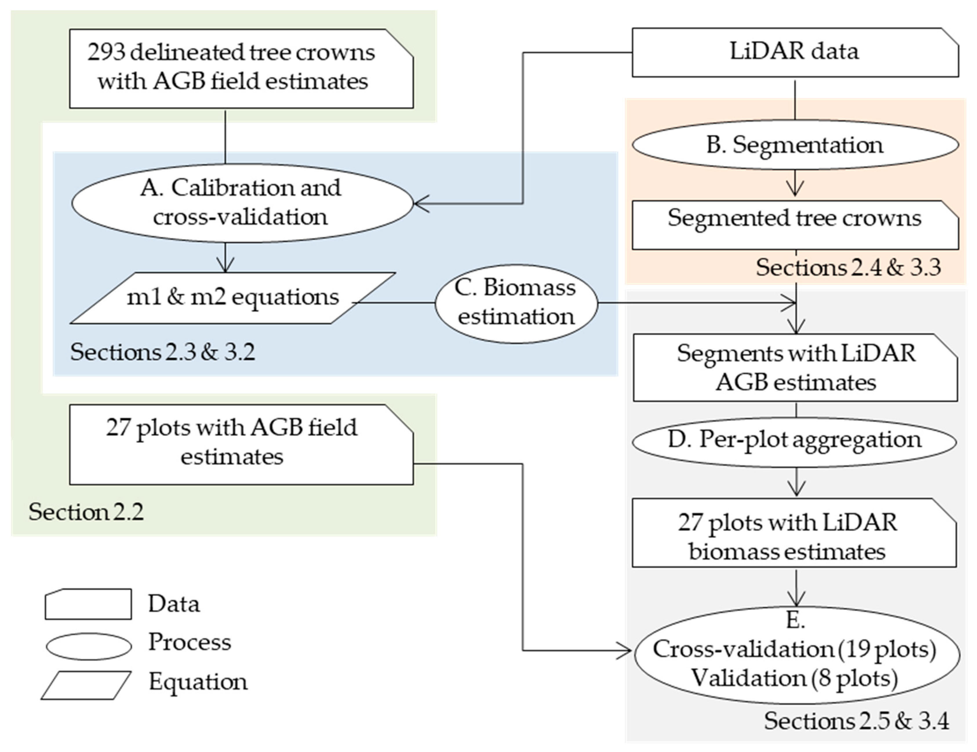
2. Materials and Methods

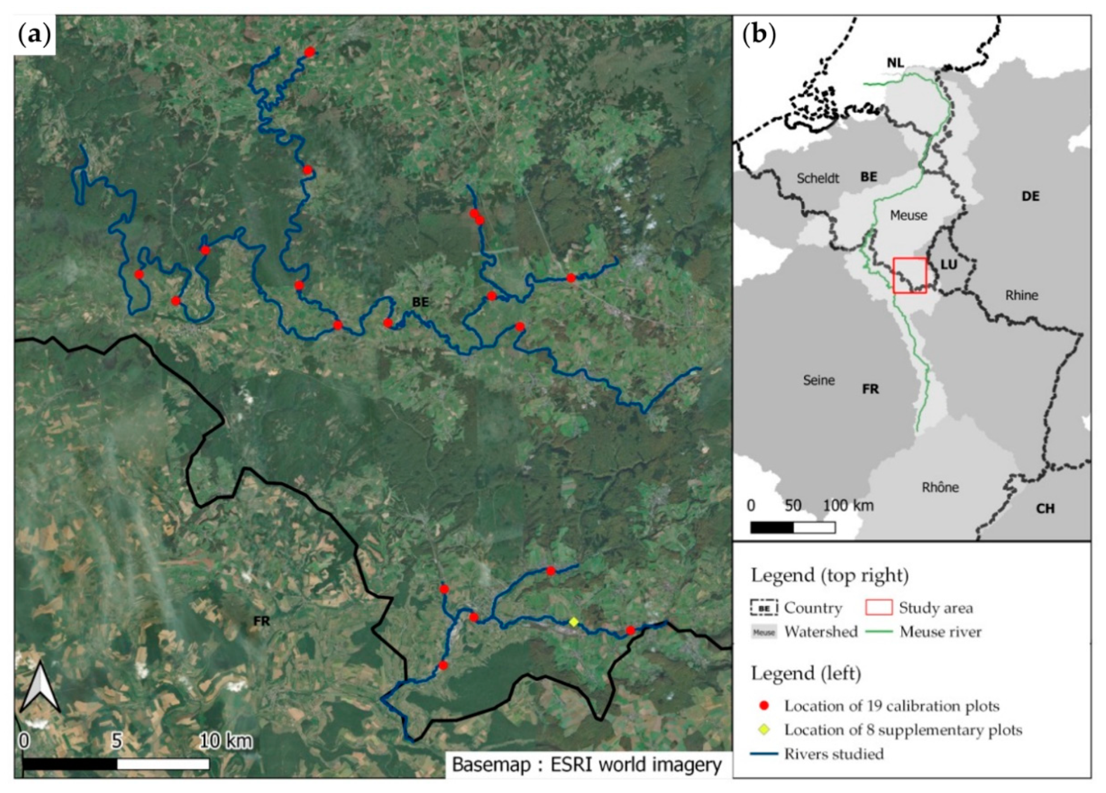
2.1. Study Area and Available Data

The study area is located in Wallonia (southern Belgium), within the Meuse catchment area (Figure 1). It is a publicly managed area, comprising about 200 km of rivers mapped from the point where their catchment area reaches 50 km2. The studied rivers drain an area of about 1200 km2. Public management in the study area is limited to the bankfull channel of rivers, as well as vegetation or other structures in the channel. It encompasses all actions needed in the channel to promote its hydraulic, ecological and social functions such as logjam removal, bank reinforcement, riparian planting, etc. The study area can be divided into two main sub-basins. In the northern part of the study area, the Semois and its tributaries have a gravel bed, a gentle slope and frequently overflow in winter. Downstream, the Semois produces broad, steeply sloping meanders [43]. In the southern part, the Ton and its tributaries have sandy beds, flow into clayey plains and have a hydrological regime dominated by base flow. On the whole, these rivers have little activity and flow in a landscape of forests and meadows, where riparian forests are often reduced to a row of trees along the river. The most frequent tree species are alders (Alnus glutinosa (L.) Gaertner) and willows (including Salix alba x fragilis L., S. viminalis L., S. caprea L. and S. aurita L.), which are often multi-stemmed. Maple (Acer pseudoplatanus L.), ash (Fraxinus excelsior L.), oak (Quercus robur L.) and hornbeam (Carpinus betulus L.) are also common. Finally, even-aged spruce plantations (Picea abies (L.) Karst) can be found in the valley bottoms.
The area was covered during the winter of 2014 by an aerial LiDAR survey. The survey was ordered by the Walloon administration over the entire Wallonia. The initial aim was to produce a DTM (Digital Terrain Model) that could then be used for multiple purposes. The acquisition was performed with a Riegl Litemapper 6800i, with a pulse repetition rate of 150 kHz and a maximum scan angle of 60°. The flight altitude ranged from 1200 to 1500 m AGL and the flight speed was 75 m/s. Average point density was 0.8 to 1 ground return/m2. Point positions were corrected during post-processing using ground references, and the mean absolute error in planimetry was 0.12 m. The point cloud was classified using full wave and morphological analysis. One-meter-resolution DTM and DSM (digital surface model) were created using a Natural Neighbor interpolation, using points classified as “ground” and points with maximum altitude, respectively. Data were provided as a point cloud with a non-normalized intensity and as 1-m-resolution DTM and DSM. A CHM was created by subtracting the DTM to the DSM. Data can be obtained on request to the Walloon public service [44].
The zone was also covered by recent (2012, 2015 and 2016) or old (several coverages since 1971) high-resolution orthophotos (<1 m). Finally, data from 17 gauging stations and models of the area flooded with a recurrence of 25 years were available throughout the area [45]. These models were produced by the regional administration using hydraulic models, hydrological statistics or field surveys, and cover the submerged areas approximately once every 25 years.

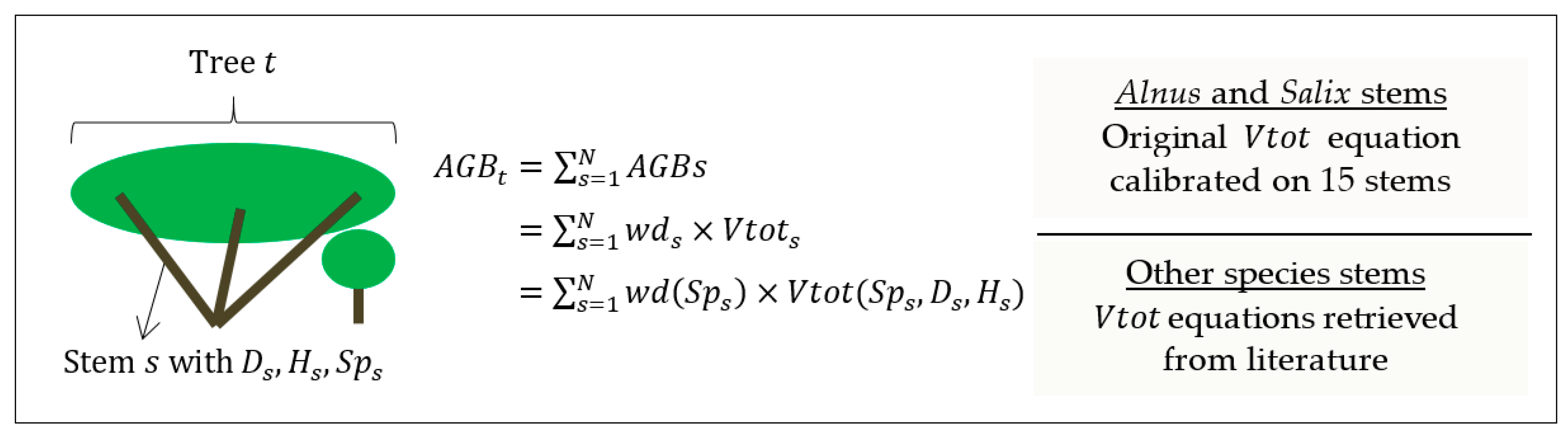
2.2. Biomass Field Data and Equations

The first step of the methodology aimed to obtain reliable biomass estimates for trees whose crown could be delineated on a LiDAR CHM. These estimates were subsequently used to calibrate a model based on LiDAR variables (see Section 2.3).
Nineteen plots were visited in 2016. Each plot was about 0.3 ha in size and located in the immediate vicinity of a river (Figure 1). While in the field, tree crowns were delineated on an orthophoto (year 2016, 25 cm in resolution) and the LiDAR CHM. Each delineated crown corresponded to the smallest unit that could be distinguished on images and linked to stems measured on the ground. A crown usually covered several stems (trees were often multi-stemmed). Species and diameter at breast height were described for all stems (DBH > 12 cm) under each crown. Stems that were not visible on aerial images were included in the crown that covered them. A total of 355 crowns were delineated, including 162 alders, 76 willows, 32 ashes, 25 maples, 18 oaks, 12 hornbeams and 32 other species.
The total wood volume of trees was estimated using volume equations for each stem separately (Figure 2). Volume equations relied on species, diameter and height data. Species and diameter were described in the field. The heights of dominant stems (whose canopies were visible from above) were estimated with the maximum height of the LiDAR CHM. The heights of suppressed stems or stems with aberrant LiDAR heights were modeled with Diameter-Height relationships, computed on other riparian trees of known height. The Diameter-Height relationship was modeled for each tree species separately using a Chapman Richards curve, which is regularly used in this context [46,47]. A different procedure was used to estimate total volume for alders and willows on one hand, and other species on the other.
Alders and willows were the two most frequently encountered genera. However, volume equations for these genera are rare and, in the case of alders, mostly limited to single-stemmed trees growing in forests managed for wood production. To estimate the total volume of these two genera, specific equations were developed on trees felled for the study. The total volume was measured by dividing the stem into two compartments: the trunk and big branches down to 12 cm in diameter on one hand, and the trunk and branches beyond the 12 cm crosscut on the other hand (see Figure S1 in Supplementary Material). Wood volume within the first compartment was measured in a traditional way, with successive diameter measures along the stem. To estimate the volume of the trunk and branches less than 12 cm in diameter, the wood contained in this compartment was shredded and the volume of shredded wood was measured. An expansion coefficient was estimated by shredding a batch of wood of known solid volume. The total volume was thus measured for 15 stems. The volume within the trunk and branches down to 12 cm in circumference was measured on 54 supplementary stems to ensure that the 15 stems selected for the total volume measurements were representative. The Equation (1), which is commonly used in tree allometry [51], was fitted using the method of least squares:
ln V t o t = a + b ×   ln D + c × ln H
where Vtot is the total wood volume, D the diameter at breast height (130 cm) and H the total height. The predictive bias associated with the log transformation was corrected by the coefficient of Baskerville [52].
To estimate the total wood volume of other species, we used regional forest trunk and stump volume equations [49] and the volume expansion factors of Longuetaud et al. [50] to estimate the total wood volume, which includes the volume of the stump, trunk and branches, following Equation (2):
V t o t = ( V d 7 × V E F + V s t u m p )
where Vd7 is the volume of the trunk until 7 cm in diameter [49], Vstump the volume of the stump [49], and VEF the volume expansion factor [50]. We systematically used double-entry equations (diameter and height), because the use of single-entry forest equations significantly overestimates the volume of riparian trees, which have a lower height than upland forest trees.
The conversion of total volume to biomass was carried out using the specific infra-density values presented in the database of Zanne et al. [48], using the equation A G B = V t o t × w d , where AGB is the tree aboveground biomass and wd the wood infra-density.
In addition, aboveground biomass was estimated in eight additional plots about 0.3 ha each, using the same methods except that tree crowns were not delineated. These eight plots were used as complementary data for validation (see Section 2.5).

2.3. Biomass Prediction from LiDAR Data at Tree Level

A tree-level allometric relationship was then adjusted between the biomass calculated in the field (in Section 2.2) and the LiDAR variables. A total of 39 trees were removed from the dataset at this stage because their crowns could not be accurately delineated. A further 23 trees were removed for other reasons, mainly because they had lost a significant part of their crown between the LiDAR and the field survey, or because they were highly distorted, and the validity of volume equations was doubtful. In the end, 293 (out of 355) trees remained. The LiDAR variables presented in Table 1 were extracted at the scale of the digitized tree crowns from the CHM and from the point cloud using the std.metrics function of the lidR R package [53].
Two parametric models were adjusted using least squares regression method. Since tree biomass can differ by several orders of magnitude, a logarithmic transformation was applied to the explanatory and response variables in order to minimize the relative error on the biomass estimate rather than the absolute error. This procedure is common for tree allometry [51]. The first model m1 (Equation (3)) was based solely on variables derived from the CHM: the area of the crown digitized by the operator (Area) and the tree height (H90) on the CHM. Several combinations of variables were tested, and the best one was chosen.
ln A G B = a + b × ln A r e a + c × ln H 90
The second model (m2) was based on variables from a CHM and from the LiDAR point cloud. After several attempts, the selected model takes the first model and adds a correction factor (Equation (4)). The first component of this correction factor is Pground, which corresponds to the proportion of returns classified as “ground” within the crown. This component has a high value for crowns that are porous to the LiDAR signal. The second component is the ratio of the height of the 30th percentile of the point cloud (Zq30) to the total crown height (H90) (Table 1). When returns are concentrated in the upper part of the canopy, this component has a high value. Together, these two factors help distinguish shade tolerant trees growing in dense forest (dense foliage concentrated in the upper crown area) from sun-demanding trees growing in full light (light foliage distributed over the entire crown). These ecological traits are worth considering because crown structure and wood density are very different along this gradient. The correction factor may also be influenced by other factors such as health status, social status or understory vegetation.
ln A G B = a + b × ln A r e a + c × ln H 90 + d × ln ( 1 + P g r o u n d 100 ) + e × ln ( 1 + Z q 30 H 90 )
These tree-level allometric models were evaluated using a leave-one-out approach, where tree crowns from 18 plots were used to calibrate a model which was then validated on the digitized tree crowns of the last plot.

2.4. Individual Tree Segmentation

Tree crowns were segmented using the algorithm of [41], implemented in the lidR package [53] and working only with a CHM. The segmentation parameters were adjusted by trial and error on a representative area. Segmentation accuracy was assessed on the 19 inventory plots by analyzing the overlaps between reference and segmented tree crowns. Two crowns corresponded when more than 50% of a reference crown was included in a segmented crown and the reference crown included more than 50% of the segmented crown [54]. The overall accuracy of the segmentation was calculated using the equation G l o b a l   a c c u r a c y = 2 × N   a c c u r a t e N   r e f e r e n c e + N   s e g m e n t e d , where N accurate is the number of corresponding tree crowns, N reference the number of manually digitized tree crowns and N segmented the number of segmented tree crowns.

2.5. Validation at Plot Level

The allometric models m1 and m2 were validated at the scale of each inventoried plot. This validation was different from the assessment carried out at the tree level because it integrated error aggregation over several crowns and the error related to segmentation (Figure 3). A leave-one-out approach was deployed. For each of the 19 plots, we adjusted the m1 and m2 allometric models based on the trees of the other 18 plots Figure 3A). On the validation plot, the trees were automatically segmented (Figure 3B) and the model built with the trees of the 18 other plots was applied to the segments Figure 3C). Tree biomasses were aggregated at plot scale (Figure 3D). The biomass estimated by remote sensing was then compared to the total biomass of the trees measured on the plot, including those that were not selected to calibrate the allometric relationship (Figure 3E). Only segments with more than half of the area within the plot were selected. A total of 8 independent plots of about 0.3 ha in which total woody biomass was known were also used for validation (see Section 2.2). The model was thus validated on a total of 27 plots.

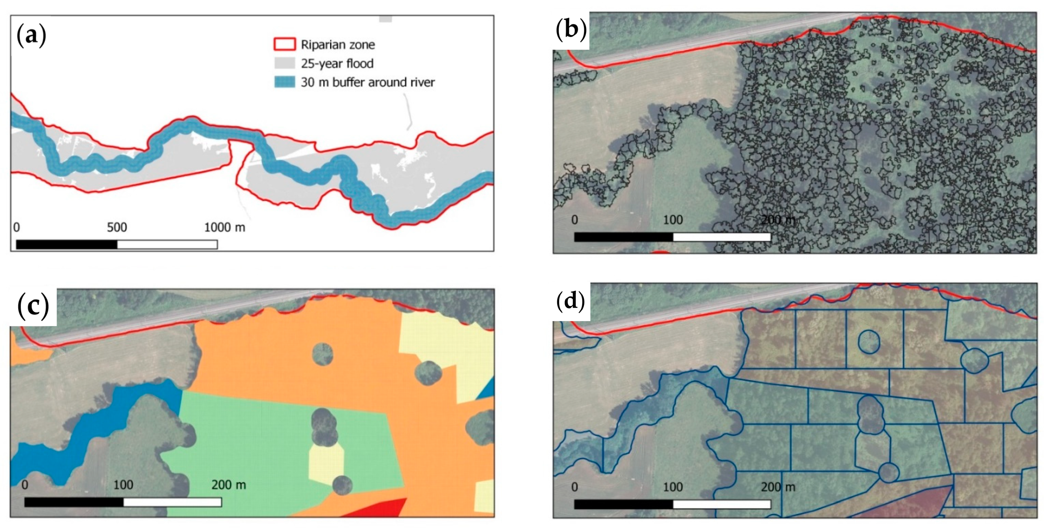
2.6. Riparian Forest Delineation and Upscaling of Biomass Prediction

The riparian zone was delineated as the area that is flooded every 25 years. This outer limit corresponds to that of zone 4 defined by Gurnell et al. [55] under a temperate climate. Beyond this limit, flooding no longer has a marked impact on ecosystem functioning. A map of the flooded area for a 25-year period was available for the entire study area (see Section 2.1). On rivers that are confined in narrow valleys, the flooded area does not always include vegetation patches that interact intensively with the river, without being periodically submerged [56]. Therefore, a fixed buffer of 30 m was delimited on both sides of the river banks. The riparian zone consists of the sum of the two envelopes: a variable buffer corresponding to the flooded area and a fixed buffer of 30 m on either side of the banks (Figure 4A). A dilation followed by an erosion of 30 m were applied to this envelope in order to eliminate small holes in the riparian zone, which have little meaning from an ecological point of view.
In this study, riparian forests were defined as native woody plant formations within the riparian zone. Segmented tree crowns were used as a starting point to delineate riparian forests (Figure 4B). Coniferous plantations (non-native to the region) and buildings, which are sometimes segmented as trees by watershed algorithms, were filtered out using an auxiliary layer at 2 m resolution previously produced at the scale of the region [57]. Tree crowns were then used to generate a “riparian forest” envelope by applying a 10-m dilation followed by a 10-m erosion. This procedure enabled the inclusion of areas that were not covered by a tree crown in plant formations where canopy is not continuous (willow thickets for example). This “riparian forest” envelope was divided into zones of homogeneous age based on historical aerial orthophotos (Figure 4C; see also Section 2.7). It was then arbitrarily divided into vegetation units (VUs) of about 0.3 ha using the “Polygon divider” tool, implemented in QGIS (Figure 4D) [58]. This area corresponds to a compromise between the finesse of the analysis (the environmental factors must be as homogeneous as possible within a VU), representativeness and validity of biomass estimates, which were validated on plots of similar size. The surface biomass of each VU (in Mg/ha) is equal to the sum of the biomasses of segmented crowns whose centroid lies within the VU, divided by the surface area of the VU. VUs less than 1000 m2 that could not be merged with another adjacent VU of similar age were excluded from the analysis to give equal weights to VUs with similar areas.

2.7. Analysis of Environmental Factors Structuring the Spatial Distribution of Biomass

To understand what environmental factors shape the spatial distribution of biomass, different explanatory variables were computed for each VU at two different scales (Table 2). At the VU scale, environmental variables were extracted at the scale of the 0.3 ha VU polygon. At the floodplain (FP) scale, the riparian zone was cut 250 m upstream and downstream of the VU, and environmental variables were extracted and summarized at the scale of the resulting polygon. Variables can be grouped into three main thematic groups: historical, land use and geomorphological variables.
Vegetation Age is presumed to be an essential variable, because many VUs in the study area result from recent colonization of agricultural areas, or have been cut down at least once during the last fifty years. Age was estimated by photo-interpretation using available orthophotos for the years 2012, 2009, 2006, 1995–1999 (several partial covers), 1983–1987 (several partial covers) and 1971. This step was performed before the final division into VUs (Figure 4c). We identified groups of contemporary trees that regenerated at the same time on historical orthophotos. The minimum size for a group of trees to be differentiated from its neighbors was 300 m2. For each group of trees, the date of vegetation regeneration was chosen as follows: when the young recruits corresponding to contemporary trees were visible on an orthophoto at a particular date, this date was retained. Otherwise, when contemporary trees appeared between two dates, the median date was chosen. As the time between two successive coverages was not constant through time, the precision was higher for young VUs (e.g., less than 3 years for trees regenerated around 2009) than for old VUs (e.g., about 14 years for trees regenerating around 1975). For trees that were already present in 1971, an age of 60 years was assigned when the trees appeared to be less than 20 years old on the 1971 orthophoto. When the vegetation seemed to already be well established, an age of 100 years was arbitrarily assigned. The trees within each VU had the same age, except for recruitment over less than 300 m2 following thinning. The type of regeneration (Planted or naturally regenerated) influences productivity in the early years, and is an important variable for managers [14]. It was therefore also described for VUs when possible, i.e., for those that regenerated after 1971.
In riparian zones, many processes related to the proximity of a river can influence biomass production. Soil Waterlogging leads to anoxia, which inhibits tree growth [61]. It was characterized using a regional soil map with five classes of waterlogging corresponding to the depth at which traces of oxidation-reduction were observed [59]. A low altitudinal position may be linked to waterlogging due to the proximity of the water table or flooding, but also increases tree growth due to water availability [62,63] and sediment input during floods [18]. It was characterized by the Vertical distance variable, which corresponds to the difference between the altitude of the VU and the altitude of the river. It was calculated following the method of Alber and Piegay [64], which was implemented in the QGIS Fluvial Corridor Toolbox [65]. The Relative vertical distance corresponds to the Vertical distance divided by the 25-year flood stage. The horizontal distance to the river (Horizontal distance) differentiates between VUs close to the current river course and subject to its direct influence, and VUs located on the old channels, where the sediments are generally finer. A high Sinuosity implies that a larger area is subject to the direct influence of the watercourse [66], and characterizes the past activity and complexity of the channel [7]. The Width of the floodplain differentiates between open, humid plains and the more shaded, steeper valleys. Catchment area is a commonly used variable that characterizes the size of the river. Finally, the terrain Slope essentially differentiates the alluvial floor from the valley slopes.
Land use is a proxy for the direct impacts of human activity on riparian vegetation. It also has an influence on light conditions or the supply of propagules. It was described using a regional land use layer from 2007, with three thematic classes: artificial areas, agricultural areas, forest areas [60]. The proportion of each land-use class was expressed in percentage area at the scale of the VU (Artificial in VU, Agriculture in VU, Forest in VU) and at the scale of the floodplain (Artificial in FP, Agriculture in FP, Forest in FP).
Explanatory variables were standardized prior to statistical analyses. A PCA (principal component analysis) was first realized in order to explore relationships between explanatory variables. A variance partition was carried out using the vegan package [67] in order to explain the share of variance in VU biomass explained by each thematic group (history, land use and geomorphology). All variables were used at this stage. A set of variables that were poorly correlated with one another (i.e., whose absolute Pearson’s correlation coefficient with other selected variables was less than 0.5) was then constituted. A MLR (multiple linear regression) model predicting VU biomass was then adjusted with the following equation:
A G B = K × A g e + ( K i × X i ) + ( k i × A g e × X i )
where Xi are explanatory variables excluding Age. The interactions of each variable with age were integrated because it was expected that the effect of the variables influencing productivity or mortality evolves with the age of vegetation. The best model was selected using a stepwise procedure based on the AIC (Akaike information criterion). The relative importance of each selected variable was computed by decomposing the explained variance into non-negative contributions, using the method of Lindeman et al. [68] implemented in the R package “relaimpo” [69].

3. Results

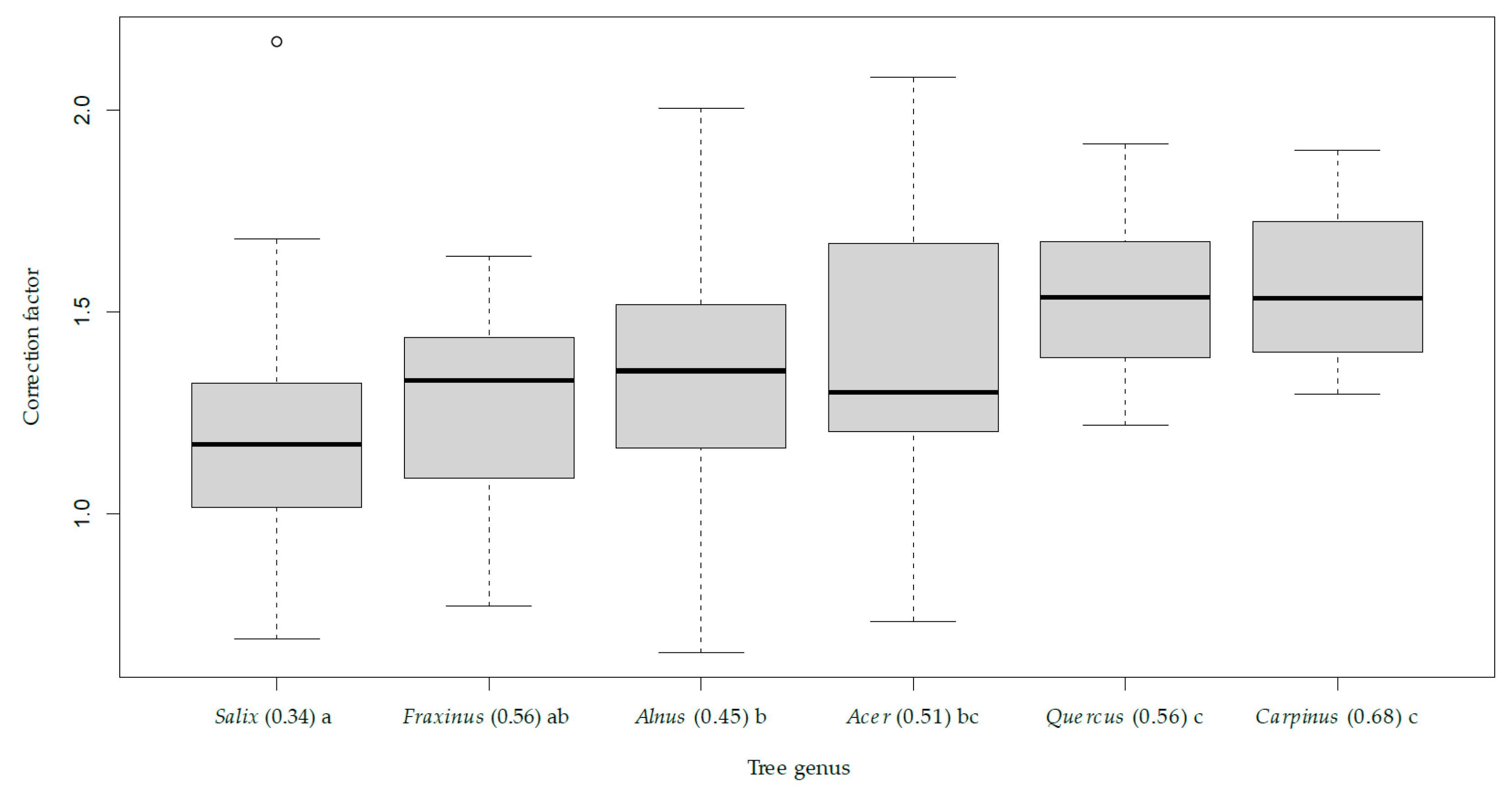
3.1. Volume Equations for Alnus and Salix

The selected model for estimating the total volume of alder and willow stems in the field is presented in Equation (6) (corresponding to the fitting of Equation (1) presented in Section 2.2). The conditions of null mean and normality of residuals, and the condition of homoscedasticity were verified respectively by a Student (p = 1), Shapiro-Wilk (p = 0.31) and Breusch Pagan test (p = 0.77). The total volume was therefore retrieved according to Equation (7), which incorporates the Baskerville correction [52].
ln V t o t = 10.8469 + 2.4079 ×   ln D + 0.7703 × ln H   ( R 2   =   0.98 ,   RMSE   =   0.16 )
V t o t = 1.9721 × 10 5 × D 2.4079 × H 0.7703
where Vtot is the total volume in cubic meters, D the diameter at breast height (1.3 m) in centimeters and H the tree height in meters.

3.2. Biomass Prediction from LiDAR Data at Tree Level

The two linear models fitted with variables from CHM (Equation (8)) and the CHM and point cloud (Equation (9)) have the following equations:
ln A G B = 9.0796 + 0.9157 × ln A r e a + 1.8354 × ln H 90   ( R 2   =   0.79 ,   RMSE   =   0.63 )
ln A G B = 8.3445 + 0.8979 × ln A r e a + 1.4880 × ln H 90 0.7951 × ln ( 1 + P g r o u n d 100 ) + 1.5534 × ln ( 1 + Z q 30 H 90 )   ( R 2   =   0.81 ,   RMSE   =   0.61 )
Deviations from application conditions were limited, and biomass was recovered by introducing a Baskerville correction [52]. M1 and m2 estimates are retrieved using Equations (10) and (11), respectively:
A G B = 1.383 × 10 4 × A r e a 0.9157 × H 90 1.8354
A G B = 2.834 × 10 4 × A r e a 0.8979 × H 90 1.4880 × ( 1 + P g r o u n d 100 ) 0.7951 × ( 1 + Z q 30 H 90 ) 1.5534
As expected, the m2 model (1.57 log-average error, corresponding to a 57% overestimation or a 36% underestimation) was slightly but significantly better than the m1 model (1.59 log-average error, corresponding to a 59% overestimation or a 37% underestimation) (Table 3).

3.3. Individual Tree Segmentation

The overall median segmentation accuracy on the reference plots was 52% (see Section 2.4 for a definition). Often several crowns were aggregated into one segment or a crown was divided into several segments, which was expected as many trees were multi-stemmed. The distribution of crowns areas was not significantly different (p = 0.82 in a Wilcoxon test) between segmented and reference (i.e., manually delineated). This close similarity justified our choice to apply calibrated allometric relationships to segments for upscaling to the whole study area.

3.4. Validation at Plot Level

The accuracy of biomass estimation at plot level was assessed using the 27 plots for m1 and m2 (Table 4 and Figure 5). As a reminder, plot aboveground biomass is equal to the sum of the biomass of all trees in the plot. Neither of the two models delivered a significantly biased biomass mean. Despite a clear improvement in R2 in m2, the models did not differ significantly in terms of absolute error (p-values of 0.44 and 0.27, respectively, for MAE (mean absolute error) and RMSE). Nevertheless, the m2 model appeared to be better than m1 for the set of criteria studied, and it was thus retained for the spatial analysis of biomass in relation to environmental factors.

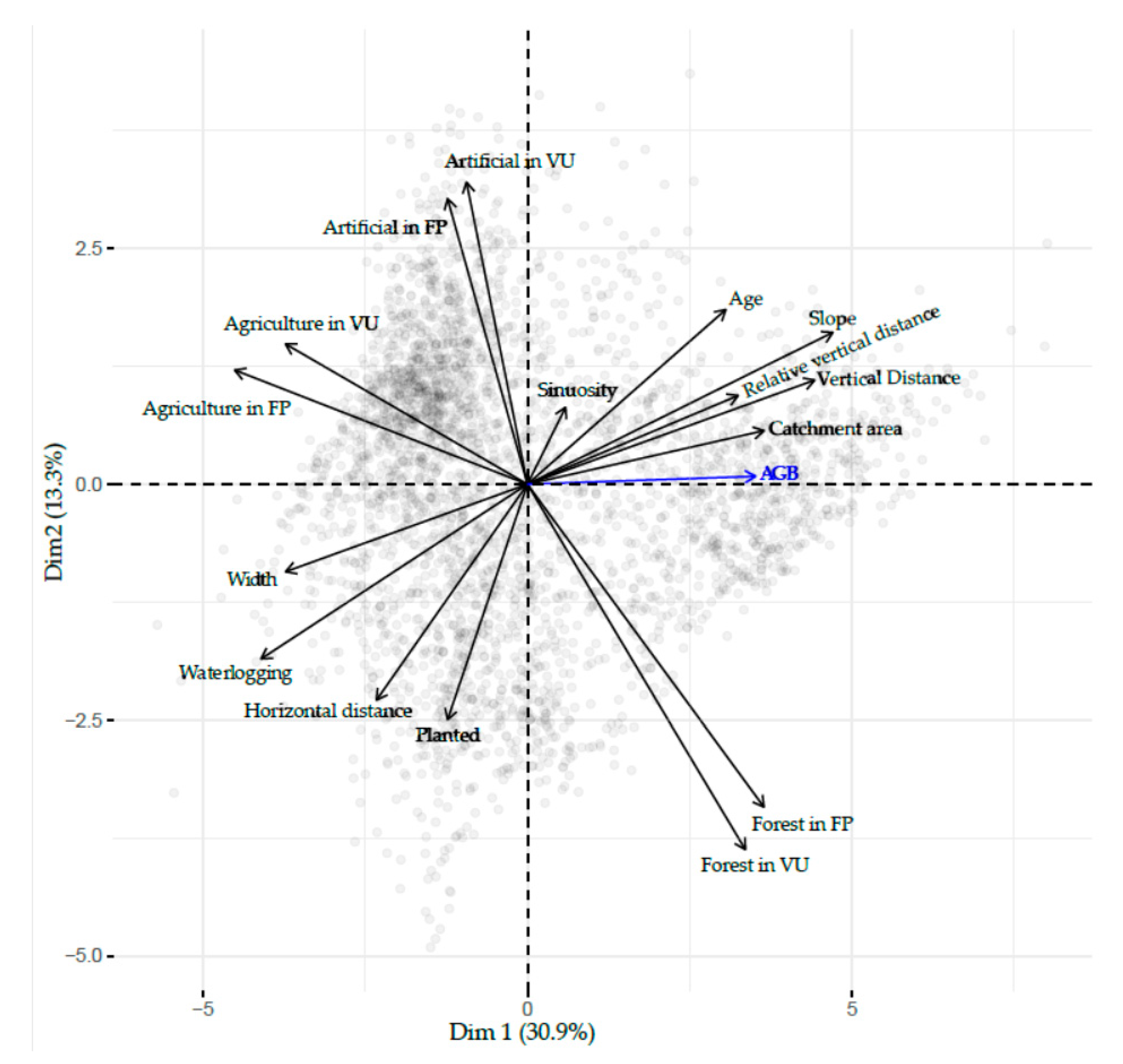
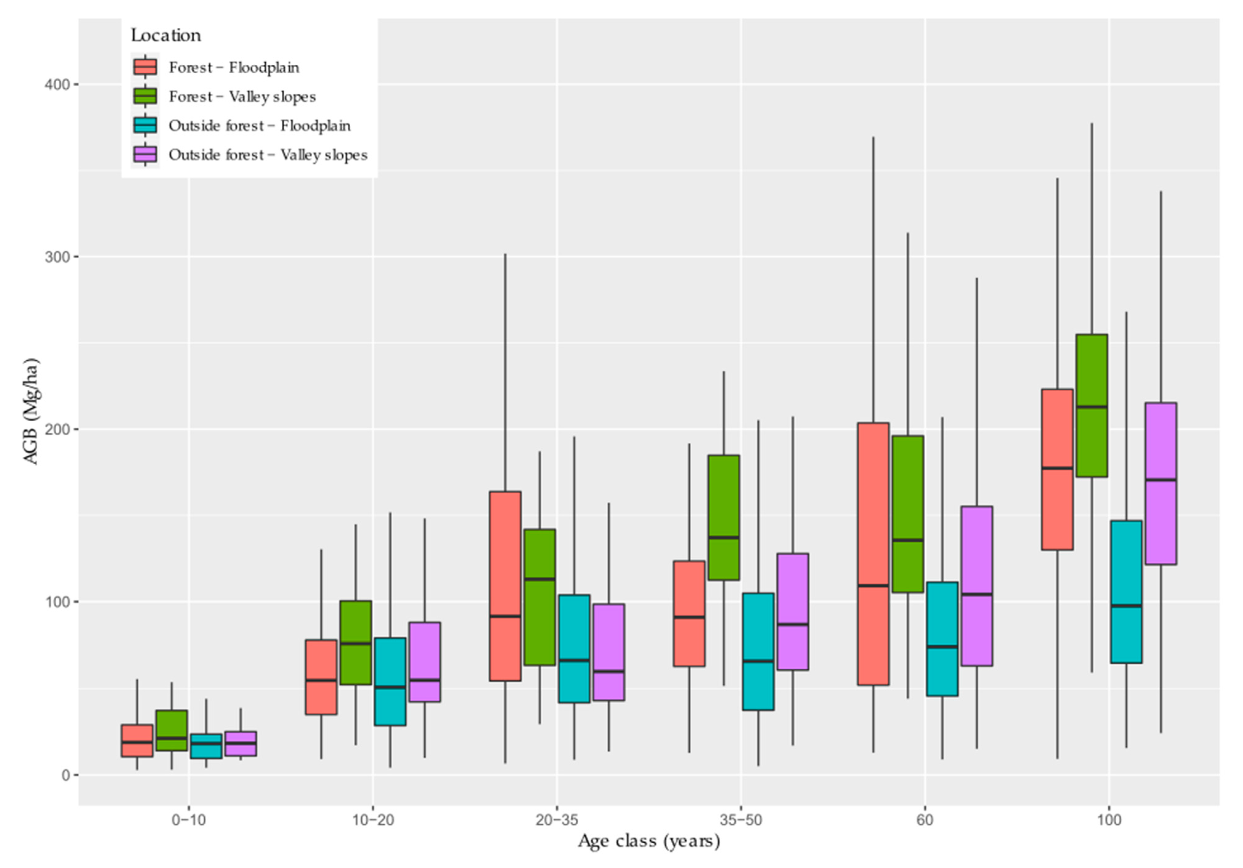
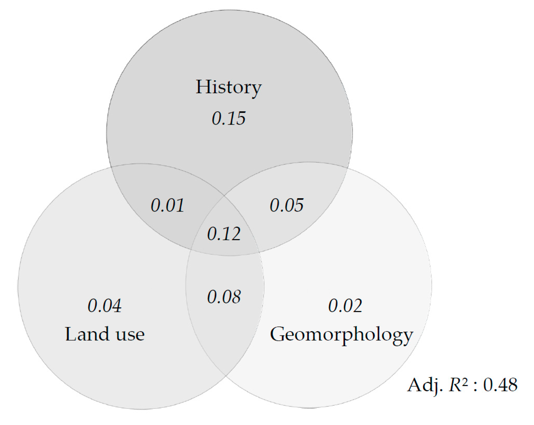
3.5. Analysis of Environmental Factors Structuring Spatial Distribution of Biomass

A total of 3162 VUs were selected for analysis. The results of a principal component analysis on explanatory variables are shown in Figure 6. Positive values on the first axis are associated with VUs occupying a higher altitudinal position, located in narrow, forested valleys, where the vegetation is older and more biomass accumulates in vegetation (high values for Vertical distance, Relative vertical distance, Slope, Age, Forest in FP and Forest in VU). Negative values are associated with VUs occupying a lower altitudinal position, located in wide, humid and predominantly agricultural valleys (high values for Agriculture in FP, Agriculture in VU, Width and Waterlogging). The second axis distinguishes the most humid VUs located in marginal depressions, in semi-open landscapes (high values for Horizontal distance, Waterlogging, Forest in FP and Forest in VU) and on the upper left the units located in more inhabited agricultural landscapes (high values for Artificial in VU and Artificial in FP).
Biomass within the VUs ranged from 3 to 515 Mg/ha (Figure 7). The average biomass for all VUs was 121 Mg/ha, and 148 Mg/ha in forested VUs (i.e., where forest land use class occupied more than 50% of the VU area). In the oldest VUs (already well established on the 1971 aerial images), the median biomass was 174 Mg/ha and 205 Mg/ha for forested VUs only. Biomass was consistently higher on valley slopes (i.e., in VUs where the relative vertical distance to the river was superior to 1) than in the floodplain (Relative vertical distance < 1).
The variance partitioning carried out with all the variables explained 48% of the variance of the biomass (Figure 8). VU history (age and regeneration type) explained 34% of the variance, present land use 25% and geomorphology 26%. Nevertheless, a large part of the variance was shared between two or all three groups of variables. The variance explained exclusively by history, land use and geomorphology were 15%, 4% and 2%, respectively. VU history was thus by far the first driver of biomass accumulation in riparian forests.
Vertical and horizontal distances to the river (Vertical distance and Horizontal distance), VU Age, Sinuosity, land use (Artificial in VU, Forest in VU, Agriculture in FP), type of regeneration (Planted) and Waterlogging variables presented Pearson’s correlation coefficients below 50%. They were thus integrated with their interactions with Age into a MLR (multiple linear regression) model predicting VU biomass. However, it must be kept in mind that variables that were removed at this stage will be accounted for by remaining, correlated variables. For example, Slope and Relative vertical distance were highly correlated with Vertical distance, and Width was highly correlated with Agriculture in FP and Horizontal distance.
The terms of the MLR model selected by a stepwise procedure are presented in Table 5. The age and the vertical distance to the river had a strong positive effect on the biomass. The percentage of forest in the VU had a strong positive effect which was strengthened by Age. Regeneration by plantation also had a positive effect strengthened by Age. It should be noted, however, that this variable always has a value of 0 for VUs older than 40 years, and therefore it has no effect on the oldest VUs. Conversely, the percentage of agriculture in the floodplain had a strong negative effect strengthened by Age. The percentage of artificialized areas in the VU and the horizontal distance to the river also had a negative impact on biomass. Finally, Sinuosity had a marginal, negative impact on biomass.

4. Discussion

4.1. LiDAR Biomass Estimates

The relative error on LiDAR biomass estimates (RMSEr of 22% on 0.3 ha plots for the m2 model) was in the lower range of the errors reported by Zolkos et al. [37] for temperate deciduous forests. These estimates are thus satisfactory, especially considering other uncertainties resulting from field data and allometric equations.
At the individual tree level, the addition of variables from the point cloud between m1 and m2 slightly improved the model. The addition of a shape and porosity factor for the crown limited the biases linked to the light conditions and the species. For example, this correction factor was significantly different depending on the species (Figure 9), and can be considered as a proxy for the heliophilous character. In a riparian context, the heliophilous character of a tree is related to its growth rate and to the density of the wood. For example, in general, Salix spp. are heliophilous, have a fast growth rate and a low wood density. When tree biomass estimates were aggregated at plot level, the added value of the variables derived from point cloud was no longer significant. However, m2 outperformed m1 in terms of R2, MAE and RMSE, and the non-significance of differences could simply be due to the small number of plots considered. Our results are thus more nuanced than those of Garcia et al. [70] and Chirici et al. [71], who found no significant difference between biomass models based on CHM or point cloud. Despite a lower performance, there are several advantages to using a model based solely on tree height and crown area. First, the use of a CHM is straightforward and does not need high computational power. The influence of survey parameters (e.g., point density, flight altitude or scan angle) or ground conditions (e.g., phenology) on CHM properties or height estimates has been well studied [53,72,73,74]. Therefore, when working simultaneously with several CHMs (e.g., multi-temporal or compiled from several locations), these effects can be accounted for or assumed to be negligible [75]. In contrast, when using point clouds, it may be more difficult to do so with variables related to lower height percentiles, canopy closure or LAI (leaf area index) [76]. A third advantage of CHMs beyond ease of use and robustness is that it can be updated with photogrammetric point clouds once a first LiDAR survey has been done [77]. The m1 model could thus be better suited to the use of time series or to the comparison of sites covered by different datasets.

4.2. Spatial Distribution of Biomass and Influencing Factors

Age was by far the most structuring variable for biomass. Moreover, as in the study of Dybala et al. [22], planting increases production in the early years compared to natural regeneration. This higher productivity of plantations was at least partially due to the choice of fast-growing species such as poplar for plantations. The median values obtained for standing biomass within forested VUs (205 Mg/ha for VUs older than 60 years, 122 Mg/ha for VUs aged 40–60 years) were within the range of values reported by for a temperate climate [5,78]. The median value obtained here for all age classes combined for forest units was 121 Mg/ha. Some authors reported very high values for all age classes, such as 284 Mg/ha for alder forests [25], or 199 Mg/ha for poplar forests and 281 Mg/ha for hardwood forests [79]. Nevertheless, these studies were carried out in smaller or protected areas, whereas the present study includes actively managed and heavily disturbed areas. Finally, the values obtained within forest units were lower than the values of aboveground woody biomass stored within forests in general in Wallonia, which are about 200 Mg/ha for deciduous forests [80]. Our lower values may be related to the lower age of the forests within the floodplain than in upland areas.
Apart from age, land use variables had a significant impact on biomass distribution. The results of variance partitioning and especially those of the MLR tended to show that the effect of land use was more important than the effect of geomorphology. In agricultural or urban areas, some VUs are regularly thinned or pruned, which can limit the accumulation of biomass. Moreover, vegetation that develops spontaneously on abandoned agricultural plots does not regenerate as quickly as in forests: the recruitment of large trees can be blocked by pioneer shrubs and is not promoted by silvicultural practices. As a result, woody recruitment is often spatially uneven or even scattered. Wasser et al. [23] also found a lower tree height in riparian corridors located in agricultural landscapes than in forested landscapes, related to higher disturbance (e.g., wind throw, mowing or plowing) and different species composition. Our results highlight the greater importance of human factors (land use and associated management practices, as well as vegetation age, which is related to human disturbance) over those of natural origin (geomorphology) in the study area. This stresses the relevance of taking into account the socio-cultural dimension of riparian ecosystems, as suggested by Dufour et al. [81].
Vegetation units in the lower parts of the riparian zone (i.e., lower vertical distance to the river) had a lower biomass at the same age than those occupying a higher topographical position. Two factors may explain this distribution. First, VUs located in lower parts of the floodplains are more heterogeneous and are subject to a more intense disturbance regime. These disturbances include flooding, erosion, and the action of beavers, which are well established throughout the area of interest. Trees in the more humid parts of the plain may also be more exposed to diseases such as Phytophtora alni [82] or Hymenoscyphus fraxineus [83]. Tree falls may also be promoted by waterlogging [84]. Apart from disturbance, waterlogging in the lower parts of the plain would have a greater impact on productivity than nutrients provided by sediment. In other studies, the balance between these two environmental variables was sometimes a dominance of the negative effect of waterlogging on productivity [16,85,86], and sometimes a dominant positive effect of nutrients or water availability [18,87]. In particular, Rodriguez-Gonzalez et al. [17] found lower radial wood growth in the wettest areas for Alnus glutinosa and Salix atrocinerea forests in the Iberian Peninsula, which are quite similar to those considered in our study. In our study, a combination of both factors—waterlogging stress and a more intense disturbance regime—explains the lower biomass found in the lower parts of the floodplain.
Finally, VUs located far from the main channel (i.e., higher horizontal distance to the river) had a lower biomass. This effect was most noticeable beyond the first fifty meters from the channel. In the study area, VUs far from the river were actually located in wide sections of the floodplain, in marginal depressions or in old channels disconnected from the river bed. These areas are enriched with fine sediments and are poorly drained. They are often occupied by shrubs such as Salix aurita, which have a low biomass.
The factors structuring riparian biomass distribution are not yet well known in most regions of the world [7]. The proposed approach could be replicated in other regions in order to compare biomass distribution patterns. For example, with a drier climate, water availability may be more limiting [88]. The response of biomass to the vertical distance to the river, which was monotonous in our study, could in these cases present a peak at intermediate altitudes as proposed by Odum [89]. It would also be possible to compare areas receiving more or less rich sediments [90], to study the distribution of biomass in other geomorphological contexts, such as in braided rivers where mortality due to erosion may be higher [91], in larger catchment areas (by going further upstream or downstream), or in less anthropized areas.

4.3. Perspectives for Generalization of the Approach

Our method essentially exploits LiDAR data, which are increasingly available at regional scales [22]. Most of the auxiliary data used are available in many countries (land use, river network) or can be derived from a LiDAR dataset (vertical distance to the river, slope, floodplain boundaries). Most countries do not have soil maps as precise as those available in Belgium, where the map is based on about two survey plots per hectare. However, soil variables seemed to be accounted for by topographical variables, and were not kept in the final MLR model. The age and type of regeneration can nevertheless be costly or tedious to obtain, as they rely on photo-interpretation of historical orthophotos, whose accessibility is uneven from one country to another.
An advantage of the individual trees approach used in this study is its flexibility regarding spatial scale. For the needs of the study, segmented trees were grouped in 0.3 ha vegetation units. However, trees can easily be re-aggregated differently depending on pursued objectives. For example, one could study biomass in the immediate vicinity of the river (e.g., first 30 m from the water edge, where bio-geomorphic interactions are most intense) using the same delineated crowns and associated biomass estimates.
We estimated only one compartment of the carbon stored by riparian ecosystems: the aboveground woody biomass. This is justified because it is the most variable compartment at a fine spatial scale and the most dynamic on time scales of a few decades [34,79]. Storage within the other compartments (especially in roots, soil and dead wood) is more difficult to measure, but it can have a significant magnitude and spatial variation, as shown by Wohl et al. [20]. These compartments are difficult to study by remote sensing, but could be modeled using topographic or geomorphological data, as in Suchenwirth et al. [34].

5. Conclusions

Our individual-tree, LiDAR-based approach enabled us to map aboveground biomass over 200 km of rivers with an error of 22% at the scale of 0.3 ha units. The addition of variables derived from the point cloud did not significantly improve CHM-based biomass estimates. For practitioners, the marginal improvement when working with point clouds must be balanced with the advantages of working with CHMs: robustness to varying survey conditions, ease of use, low computational requirements and possible update with photogrammetric point clouds.
The biomass map was used to better understand the patterns of biomass distribution within the riparian zone. In the study area, vegetation age was the most important variable. Present land use was second, followed by geomorphological variables. Over the study area, anthropogenic factors (land use and vegetation age, which are related to human practices) were more important than geomorphic factors concerning biomass accumulation within vegetation.
Surface biomass was higher inside forest, in higher topographical parts of the riparian zone and close to the river rather than in remnant patches in the agricultural landscape, and in low-lying areas further away from the river. The implementation of similar approaches in other catchments will be eased by the growing availability of LiDAR data at regional scales. Ultimately, remote sensing approaches could help understand how spatial biomass distribution patterns vary depending on the ecological context, and inform land use, conservation or restoration policies in riparian zones.

Supplementary Materials

The following are available online at https://www.mdpi.com/1999-4907/12/3/371/s1, Figure S1: Estimation of total wood volume.

Author Contributions

Conceptualization, L.H., A.M., N.L. and P.L.; methodology, L.H., A.M. and N.L.; software, L.H. and A.M.; formal analysis, L.H.; data curation, L.H.; writing—original draft preparation, L.H.; writing—review and editing, L.H., A.M., N.L., P.L., H.C., B.G.; supervision, A.M. and P.L. All authors have read and agreed to the published version of the manuscript.

Funding

This work received financial support from the Province of Liège and the Province of Luxembourg.

Institutional Review Board Statement

Not applicable.

Informed Consent Statement

Not applicable.

Data Availability Statement

Original data created in this study including VUs with associated AGB and explanatory variables and calibration measures for alder/willow field volume equations are available at Mendeley Data (doi: 10.17632/ydrkfw9r84.1). Other data are available from the corresponding author upon reasonable request.

Acknowledgments

Measurements for Alnus/Salix field volume equations were made possible by the Service Public Wallonie—Direction des Cours d’eau non navigables.

Conflicts of Interest

The authors declare no conflict of interest.

References

  1. Naiman, R.J.; Decamps, H.; Pollock, M. The Role of Riparian Corridors in Maintaining Regional Biodiversity. Ecol. Appl. 1993, 3, 209–212. [Google Scholar] [CrossRef]
  2. Riis, T.; Kelly-Quinn, M.; Aguiar, F.C.; Manolaki, P.; Bruno, D.; Bejarano, M.D.; Clerici, N.; Fernandes, M.R.; Franco, J.C.; Pettit, N.; et al. Global Overview of Ecosystem Services Provided by Riparian Vegetation. BioScience 2020, 70, 501–514. [Google Scholar] [CrossRef]
  3. Stella, J.C.; Bendix, J. Chapter 5Multiple Stressors in Riparian Ecosystems. In Multiple Stressors in River Ecosystems; Sabater, S., Elosegi, A., Ludwig, R., Eds.; Elsevier: Amsterdam, The Netherlands, 2019; pp. 81–110. ISBN 978-0-12-811713-2. [Google Scholar] [CrossRef]
  4. González, E.; Sher, A.A.; Tabacchi, E.; Masip, A.; Poulin, M. Restoration of riparian vegetation: A global review of implementation and evaluation approaches in the international, peer-reviewed literature. J. Environ. Manag. 2015, 158, 85–94. [Google Scholar] [CrossRef] [PubMed]
  5. Dybala, K.E.; Matzek, V.; Gardali, T.; Seavy, N.E. Carbon sequestration in riparian forests: A global synthesis and meta-analysis. Glob. Chang. Biol. 2019, 25, 57–67. [Google Scholar] [CrossRef] [PubMed] [Green Version]
  6. Matzek, V.; Stella, J.; Ropion, P. Development of a carbon calculator tool for riparian forest restoration. Appl. Veg. Sci. 2018, 21, 584–594. [Google Scholar] [CrossRef]
  7. Sutfin, N.A.; Wohl, E.E.; Dwire, K.A. Banking carbon: A review of organic carbon storage and physical factors influencing retention in floodplains and riparian ecosystems. Earth Surf. Process. Landf. 2016, 41, 38–60. [Google Scholar] [CrossRef]
  8. Balian, E.V.; Naiman, R.J. Abundance and Production of Riparian Trees in the Lowland Floodplain of the Queets River, Washington. Ecosystems 2005, 8, 841–861. [Google Scholar] [CrossRef]
  9. Keeton, W.S.; Kraft, C.E.; Warren, D.R. Mature and Old-Growth Riparian Forests: Structure, Dynamics, and Effects on Adirondack Stream Habitats. Ecol. Appl. 2007, 17, 852–868. [Google Scholar] [CrossRef]
  10. Dosskey, M.G.; Vidon, P.; Gurwick, N.P.; Allan, C.J.; Duval, T.P.; Lowrance, R. The Role of Riparian Vegetation in Protecting and Improving Chemical Water Quality in Streams1. JAWRA J. Am. Water Resour. Assoc. 2010, 46, 261–277. [Google Scholar] [CrossRef]
  11. Tufekcioglu, A.; Raich, J.W.; Isenhart, T.M.; Schultz, R.C. Biomass, carbon and nitrogen dynamics of multi-species riparian buffers within an agricultural watershed in Iowa, USA. Agrofor. Syst. 2003, 57, 187–198. [Google Scholar] [CrossRef]
  12. Matzek, V.; Lewis, D.; O’Geen, A.; Lennox, M.; Hogan, S.D.; Feirer, S.T.; Eviner, V.; Tate, K.W. Increases in soil and woody biomass carbon stocks as a result of rangeland riparian restoration. Carbon Balance Manag. 2020, 15, 16. [Google Scholar] [CrossRef] [PubMed]
  13. Forzieri, G.; Castelli, F.; Preti, F. Advances in remote sensing of hydraulic roughness. Int. J. Remote Sens. 2012, 33, 630–654. [Google Scholar] [CrossRef]
  14. Dybala, K.E.; Steger, K.; Walsh, R.G.; Smart, D.R.; Gardali, T.; Seavy, N.E. Optimizing carbon storage and biodiversity co-benefits in reforested riparian zones. J. Appl. Ecol. 2019, 56, 343–353. [Google Scholar] [CrossRef]
  15. Dufour, S.; Piégay, H. Geomorphological Controls of Fraxinus Excelsior Growth and Regeneration in Floodplain Forests. Ecology 2008, 89, 205–215. [Google Scholar] [CrossRef]
  16. Megonigal, J.P.; Conner, W.H.; Kroeger, S.; Sharitz, R.R. Aboveground Production in Southeastern Floodplain Forests: A Test of the Subsidy–Stress Hypothesis. Ecology 1997, 78, 370–384. [Google Scholar] [CrossRef] [Green Version]
  17. Rodríguez-González, P.M.; Stella, J.C.; Campelo, F.; Ferreira, M.T.; Albuquerque, A. Subsidy or stress? Tree structure and growth in wetland forests along a hydrological gradient in Southern Europe. For. Ecol. Manag. 2010, 259, 2015–2025. [Google Scholar] [CrossRef]
  18. Marks, C.O.; Yellen, B.C.; Wood, S.A.; Martin, E.H.; Nislow, K.H. Variation in Tree Growth along Soil Formation and Microtopographic Gradients in Riparian Forests. Wetlands 2020. [Google Scholar] [CrossRef]
  19. Kramer, K.; Vreugdenhil, S.J.; van der Werf, D.C. Effects of flooding on the recruitment, damage and mortality of riparian tree species: A field and simulation study on the Rhine floodplain. For. Ecol. Manag. 2008, 255, 3893–3903. [Google Scholar] [CrossRef]
  20. Wohl, E.; Dwire, K.; Sutfin, N.; Polvi, L.; Bazan, R. Mechanisms of carbon storage in mountainous headwater rivers. Nat. Commun. 2012, 3, 1263. [Google Scholar] [CrossRef] [Green Version]
  21. Lucas, C.M.; Schöngart, J.; Sheikh, P.; Wittmann, F.; Piedade, M.T.F.; McGrath, D.G. Effects of land-use and hydroperiod on aboveground biomass and productivity of secondary Amazonian floodplain forests. For. Ecol. Manag. 2014, 319, 116–127. [Google Scholar] [CrossRef]
  22. Michez, A.; Piégay, H.; Lejeune, P.; Claessens, H. Multi-temporal monitoring of a regional riparian buffer network (>12,000 km) with LiDAR and photogrammetric point clouds. J. Environ. Manag. 2017, 202, 424–436. [Google Scholar] [CrossRef] [PubMed]
  23. Wasser, L.; Chasmer, L.; Day, R.; Taylor, A. Quantifying land use effects on forested riparian buffer vegetation structure using LiDAR data. Ecosphere 2015, 6, art10. [Google Scholar] [CrossRef]
  24. da Silva, R.L.; Leite, M.F.A.; Muniz, F.H.; de Souza, L.A.G.; de Moraes, F.H.R.; Gehring, C. Degradation impacts on riparian forests of the lower Mearim river, eastern periphery of Amazonia. For. Ecol. Manag. 2017, 402, 92–101. [Google Scholar] [CrossRef]
  25. Fernandes, M.R.; Aguiar, F.C.; Martins, M.J.; Rico, N.; Ferreira, M.T.; Correia, A.C. Carbon Stock Estimations in a Mediterranean Riparian Forest: A Case Study Combining Field Data and UAV Imagery. Forests 2020, 11, 376. [Google Scholar] [CrossRef] [Green Version]
  26. Lu, D. The potential and challenge of remote sensing-based biomass estimation. Int. J. Remote Sens. 2006, 27, 1297–1328. [Google Scholar] [CrossRef]
  27. Goetz, S.; Dubayah, R. Advances in remote sensing technology and implications for measuring and monitoring forest carbon stocks and change. Carbon Manag. 2011, 2, 231–244. [Google Scholar] [CrossRef]
  28. Huylenbroeck, L.; Laslier, M.; Dufour, S.; Georges, B.; Lejeune, P.; Michez, A. Using remote sensing to characterize riparian vegetation: A review of available tools and perspectives for managers. J. Environ. Manag. 2020, 267, 110652. [Google Scholar] [CrossRef]
  29. Mendez-Estrella, R.; Romo-Leon, J.R.; Castellanos, A.E. Mapping Changes in Carbon Storage and Productivity Services Provided by Riparian Ecosystems of Semi-Arid Environments in Northwestern Mexico. ISPRS Int. J. Geo Inf. 2017, 6, 298. [Google Scholar] [CrossRef]
  30. Husson, E.; Lindgren, F.; Ecke, F. Assessing Biomass and Metal Contents in Riparian Vegetation Along a Pollution Gradient Using an Unmanned Aircraft System. Water Air Soil Pollut. 2014, 225, 1957. [Google Scholar] [CrossRef]
  31. Mitchard, E.T.A.; Saatchi, S.S.; White, L.J.T.; Abernethy, K.A.; Jeffery, K.J.; Lewis, S.L.; Collins, M.; Lefsky, M.A.; Leal, M.E.; Woodhouse, I.H.; et al. Mapping tropical forest biomass with radar and spaceborne LiDAR in Lopé National Park, Gabon: Overcoming problems of high biomass and persistent cloud. Biogeosciences 2012, 9, 179–191. [Google Scholar] [CrossRef] [Green Version]
  32. Filippi, A.M.; Güneralp, İ.; Randall, J. Hyperspectral remote sensing of aboveground biomass on a river meander bend using multivariate adaptive regression splines and stochastic gradient boosting. Remote Sens. Lett. 2014, 5, 432–441. [Google Scholar] [CrossRef]
  33. Forzieri, G. Satellite retrieval of woody biomass for energetic reuse of riparian vegetation. Biomass Bioenergy 2012, 36, 432–438. [Google Scholar] [CrossRef]
  34. Suchenwirth, L.; Stümer, W.; Schmidt, T.; Förster, M.; Kleinschmit, B. Large-Scale Mapping of Carbon Stocks in Riparian Forests with Self-Organizing Maps and the k-Nearest-Neighbor Algorithm. Forests 2014, 5, 1635–1652. [Google Scholar] [CrossRef] [Green Version]
  35. Fassnacht, F.E.; Hartig, F.; Latifi, H.; Berger, C.; Hernández, J.; Corvalán, P.; Koch, B. Importance of sample size, data type and prediction method for remote sensing-based estimations of aboveground forest biomass. Remote Sens. Environ. 2014, 154, 102–114. [Google Scholar] [CrossRef]
  36. Laslier, M.; Hubert-Moy, L.; Dufour, S. Mapping Riparian Vegetation Functions Using 3D Bispectral LiDAR Data. Water 2019, 11, 483. [Google Scholar] [CrossRef] [Green Version]
  37. Zolkos, S.G.; Goetz, S.J.; Dubayah, R. A meta-analysis of terrestrial aboveground biomass estimation using lidar remote sensing. Remote Sens. Environ. 2013, 128, 289–298. [Google Scholar] [CrossRef]
  38. Cartisano, R.; Mattioli, W.; Corona, P.; Mugnozza, G.S.; Sabatti, M.; Ferrari, B.; Cimini, D.; Giuliarelli, D. Assessing and mapping biomass potential productivity from poplar-dominated riparian forests: A case study. Biomass Bioenergy 2013, 54, 293–302. [Google Scholar] [CrossRef] [Green Version]
  39. Karrenberg, S.; Edwards, P.J.; Kollmann, J. The life history of Salicaceae living in the active zone of floodplains. Freshw. Biol. 2002, 47, 733–748. [Google Scholar] [CrossRef]
  40. Naiman, R.J.; Decamps, H.; McClain, M.E. Riparia: Ecology, Conservation, and Management of Streamside Communities; Elsevier: Amsterdam, The Netherlands, 2005; ISBN 978-0-08-047068-9. [Google Scholar]
  41. Dalponte, M.; Coomes, D.A. Tree-centric mapping of forest carbon density from airborne laser scanning and hyperspectral data. Methods Ecol. Evol. 2016, 7, 1236–1245. [Google Scholar] [CrossRef] [Green Version]
  42. Cadol, D.; Wine, M.L. Geomorphology as a first order control on the connectivity of riparian ecohydrology. Geomorphology 2017, 277, 154–170. [Google Scholar] [CrossRef]
  43. Gob, F.; Houbrechts, G.; Hiver, J.M.; Petit, F. River dredging, channel dynamics and bedload transport in an incised meandering river (the River Semois, Belgium). River Res. Appl. 2005, 21, 791–804. [Google Scholar] [CrossRef]
  44. Service Public Wallonie. Nuage de Points LIDAR 2013–2014. Available online: http://geoportail.wallonie.be/catalogue/cd7578ef-c726-46cb-a29e-a90b3d4cd368.html (accessed on 5 March 2021).
  45. Service Public Wallonie. Notice Méthodologique D’élaboration des Cartographies des Zones Soumises À L’aléa D’inondation et du Risque de Dommages dus Aux Inondations. Available online: http://environnement.wallonie.be/inondations/files/2016_carto/Methodo_GW20160310_final.pdf (accessed on 14 December 2020).
  46. Corral-Rivas, S.; Álvarez-González, J.G.; Crecente-Campo, F.; Corral-Rivas, J.J. Local and generalized height-diameter models with random parameters for mixed, uneven-aged forests in Northwestern Durango, Mexico. For. Ecosyst. 2014, 1, 6. [Google Scholar] [CrossRef] [Green Version]
  47. Ahmadi, K.; Alavi, S.J.; Kouchaksaraei, M.T. Constructing site quality curves and productivity assessment for uneven-aged and mixed stands of oriental beech (Fagus oriental Lipsky) in Hyrcanian forest, Iran. For. Sci. Technol. 2017, 13, 41–46. [Google Scholar] [CrossRef]
  48. Zanne, A.; Lopez-Gonzalez, G.; Coomes, D.; Ilic, J.; Jansen, S.; Lewis, S.; Miller, R.; Swenson, N.; Wiemann, M.; Chave, J. Data from: Towards a worldwide wood economics spectrum. Dryad Digit Repos. Dryad 2009. [Google Scholar] [CrossRef]
  49. Dagnelie, P.; Palm, R.; Rondeux, J. Cubage des Arbres et des Peuplements Forestiers. Tables et Équations; Presses Agronomiques de Gembloux: Gembloux, Belgium, 2013. [Google Scholar]
  50. Longuetaud, F.; Santenoise, P.; Mothe, F.; Senga Kiessé, T.; Rivoire, M.; Saint-André, L.; Ognouabi, N.; Deleuze, C. Modeling volume expansion factors for temperate tree species in France. For. Ecol. Manag. 2013, 292, 111–121. [Google Scholar] [CrossRef]
  51. Zianis, D.; Muukkonen, P.; Mäkipää, R.; Mencuccini, M. Biomass and Stem Volume Equations for Tree Species in Europe; Finnish Society of Forest Science: Helsinki, Finland, 2005; ISBN 978-951-40-1983-8. [Google Scholar]
  52. Baskerville, G.L. Use of Logarithmic Regression in the Estimation of Plant Biomass. Can. J. For. Res. 2011. [Google Scholar] [CrossRef]
  53. Roussel, J.-R.; Auty, D.; De Boissieu, F.; Sánchez Meador, A.; Bourdon, J.-F.; Gatziolis, D. lidR: Airborne LiDAR Data Manipulation and Visualization for Forestry Applications. 2020; R package, version 2.2.4. [Google Scholar]
  54. Lamar, W.R.; McGraw, J.B.; Warner, T.A. Multitemporal censusing of a population of eastern hemlock (Tsuga canadensis L.) from remotely sensed imagery using an automated segmentation and reconciliation procedure. Remote Sens. Environ. 2005, 94, 133–143. [Google Scholar] [CrossRef]
  55. Gurnell, A.M.; Corenblit, D.; de Jalón, D.G.; del Tánago, M.G.; Grabowski, R.C.; O’Hare, M.T.; Szewczyk, M. A Conceptual Model of Vegetation–hydrogeomorphology Interactions Within River Corridors. River Res. Appl. 2016, 32, 142–163. [Google Scholar] [CrossRef]
  56. Clerici, N.; Weissteiner, C.J.; Paracchini, M.L.; Boschetti, L.; Baraldi, A.; Strobl, P. Pan-European distribution modelling of stream riparian zones based on multi-source Earth Observation data. Ecol. Indic. 2013, 24, 211–223. [Google Scholar] [CrossRef]
  57. Radoux, J.; Bourdouxhe, A.; Coos, W.; Dufrêne, M.; Defourny, P. Improving Ecotope Segmentation by Combining Topographic and Spectral Data. Remote Sens. 2019, 11, 354. [Google Scholar] [CrossRef] [Green Version]
  58. Huck, J. jonnyhuck/RFCL-PolygonDivider. 2020; QGIS plugin, version 0.6. [Google Scholar]
  59. Service Public Wallonie. Carte Numérique des Sols de Wallonie—Série. Available online: http://geoportail.wallonie.be/catalogue/c5bedf2b-1cac-4231-9d9a-854e0ef2c9ce.html (accessed on 15 December 2020).
  60. Service Public Wallonie. Occupation et Utilisation du sol en Wallonie—COSW 2007—Série—Donnée Historique. Available online: http://geoportail.wallonie.be/catalogue/290e1fe8-0d99-410e-967b-a02f389b931a.html (accessed on 14 December 2020).
  61. Kreuzwieser, J.; Papadopoulou, E.; Rennenberg, H. Interaction of Flooding with Carbon Metabolism of Forest Trees. Plant Biol. 2004, 6, 299–306. [Google Scholar] [CrossRef]
  62. Singer, M.B.; Stella, J.C.; Dufour, S.; Piégay, H.; Wilson, R.J.S.; Johnstone, L. Contrasting water-uptake and growth responses to drought in co-occurring riparian tree species. Ecohydrology 2013, 6, 402–412. [Google Scholar] [CrossRef]
  63. Schifman, L.A.; Stella, J.C.; Volk, T.A.; Teece, M.A. Carbon isotope variation in shrub willow (Salix spp.) ring-wood as an indicator of long-term water status, growth and survival. Biomass Bioenergy 2012, 36, 316–326. [Google Scholar] [CrossRef]
  64. Alber, A.; Piégay, H. Spatial disaggregation and aggregation procedures for characterizing fluvial features at the network-scale: Application to the Rhône basin (France). Geomorphology 2011, 125, 343–360. [Google Scholar] [CrossRef]
  65. Christophe, R.; Samuel, D. Fluvial Corridor Toolbox QGis Plugin; Zenodo: Genève, Switzerland, 2020. [Google Scholar] [CrossRef]
  66. Camporeale, C.; Ridolfi, L. Interplay among river meandering, discharge stochasticity and riparian vegetation. J. Hydrol. 2010, 382, 138–144. [Google Scholar] [CrossRef]
  67. Oksanen, J.; Blanchet, F.G.; Friendly, M.; Kindt, R.; Legendre, P.; McGlinn, D.; Minchin, P.R.; O’Hara, R.B.; Simpson, G.L.; Solymos, P.; et al. Vegan: Community Ecology Package. 2020; R package, version 2.5-7. [Google Scholar]
  68. Lindeman, R.; Merenda, P.; Gold, R. Introduction to Bivariate and Multivariate Analysis; Scott Foresman: Chicago, IL, USA, 1980. [Google Scholar]
  69. Groemping, U.; Lehrkamp, M. Relaimpo: Relative Importance of Regressors in Linear Models. 2018; R package, version 2.2-3. [Google Scholar]
  70. Garcia, M.; Saatchi, S.; Ferraz, A.; Silva, C.A.; Ustin, S.; Koltunov, A.; Balzter, H. Impact of data model and point density on aboveground forest biomass estimation from airborne LiDAR. Carbon Balance Manag. 2017, 12, 4. [Google Scholar] [CrossRef] [PubMed] [Green Version]
  71. Chirici, G.; McRoberts, R.E.; Fattorini, L.; Mura, M.; Marchetti, M. Comparing echo-based and canopy height model-based metrics for enhancing estimation of forest aboveground biomass in a model-assisted framework. Remote Sens. Environ. 2016, 174, 1–9. [Google Scholar] [CrossRef]
  72. Holmgren, J.; Nilsson, M.; Olsson, H. Simulating the effects of lidar scanning angle for estimation of mean tree height and canopy closure. Can. J. Remote Sens. 2003, 29, 623–632. [Google Scholar] [CrossRef]
  73. Nasset, E. Effects of different flying altitudes on biophysical stand properties estimated from canopy height and density measured with a small-footprint airborne scanning laser. Remote Sens. Environ. 2004, 91, 243–255. [Google Scholar] [CrossRef]
  74. Zhao, K.; Suarez, J.C.; Garcia, M.; Hu, T.; Wang, C.; Londo, A. Utility of multitemporal lidar for forest and carbon monitoring: Tree growth, biomass dynamics, and carbon flux. Remote Sens. Environ. 2018, 204, 883–897. [Google Scholar] [CrossRef]
  75. Duncanson, L.; Dubayah, R. Monitoring individual tree-based change with airborne lidar. Ecol. Evol. 2018, 8, 5079–5089. [Google Scholar] [CrossRef] [PubMed]
  76. Liu, J.; Skidmore, A.K.; Jones, S.; Wang, T.; Heurich, M.; Zhu, X.; Shi, Y. Large off-nadir scan angle of airborne LiDAR can severely affect the estimates of forest structure metrics. ISPRS J. Photogramm. Remote Sens. 2018, 136, 13–25. [Google Scholar] [CrossRef]
  77. Michez, A.; Huylenbroeck, L.; Bolyn, C.; Latte, N.; Bauwens, S.; Lejeune, P. Can regional aerial images from orthophoto surveys produce high quality photogrammetric Canopy Height Model? A single tree approach in Western Europe. Int. J. Appl. Earth Obs. Geoinf. 2020, 92, 102190. [Google Scholar] [CrossRef]
  78. Giese, L.A.B.; Aust, W.M.; Kolka, R.K.; Trettin, C.C. Biomass and carbon pools of disturbed riparian forests. For. Ecol. Manag. 2003, 180, 493–508. [Google Scholar] [CrossRef]
  79. Cierjacks, A.; Kleinschmit, B.; Babinsky, M.; Kleinschroth, F.; Markert, A.; Menzel, M.; Ziechmann, U.; Schiller, T.; Graf, M.; Lang, F. Carbon stocks of soil and vegetation on Danubian floodplains. J. Plant Nutr. Soil Sci. 2010, 173, 644–653. [Google Scholar] [CrossRef]
  80. Latte, N.; Colinet, G.; Fayolle, A.; Lejeune, P.; Hébert, J.; Claessens, H.; Bauwens, S. Description of a new procedure to estimate the carbon stocks of all forest pools and impact assessment of methodological choices on the estimates. Eur. J. For. Res. 2013, 132, 565–577. [Google Scholar] [CrossRef] [Green Version]
  81. Dufour, S.; Rodríguez-González, P.M.; Laslier, M. Tracing the scientific trajectory of riparian vegetation studies: Main topics, approaches and needs in a globally changing world. Sci. Total Environ. 2019, 653, 1168–1185. [Google Scholar] [CrossRef]
  82. Strnadová, V.; Černý, K.; Holub, V.; Gregorová, B. The effects of flooding and Phytophthora alni infection on black alder. J. For. Sci. 2010, 56, 6. [Google Scholar] [CrossRef] [Green Version]
  83. Marçais, B.; Husson, C.; Godart, L.; Caël, O. Influence of site and stand factors on Hymenoscyphus fraxineus-induced basal lesions. Plant Pathol. 2016, 65, 1452–1461. [Google Scholar] [CrossRef]
  84. Ferry, B.; Morneau, F.; Bontemps, J.-D.; Blanc, L.; Freycon, V. Higher treefall rates on slopes and waterlogged soils result in lower stand biomass and productivity in a tropical rain forest. J. Ecol. 2010, 98, 106–116. [Google Scholar] [CrossRef]
  85. Cavalcanti, G.G.; Lockaby, B.G. Effects of sediment deposition on aboveground net primary productivity, vegetation composition, and structure in riparian forests. Wetlands 2006, 26, 400–409. [Google Scholar] [CrossRef]
  86. Jolley, R.L.; Lockaby, B.G.; Cavalcanti, G.G. Productivity of Ephemeral Headwater Riparian Forests Impacted by Sedimentation in the Southeastern United States Coastal Plain. J. Environ. Qual. 2009, 38, 965–979. [Google Scholar] [CrossRef] [PubMed]
  87. Clawson, R.G.; Lockaby, B.G.; Rummer, B. Changes in Production and Nutrient Cycling across a Wetness Gradient within a Floodplain Forest. Ecosystems 2001, 4, 126–138. [Google Scholar] [CrossRef]
  88. Amlin, N.M.; Rood, S.B. Drought stress and recovery of riparian cottonwoods due to water table alteration along Willow Creek, Alberta. Trees 2003, 17, 351–358. [Google Scholar] [CrossRef]
  89. Odum, E.P.; Finn, J.T.; Franz, E.H. Perturbation Theory and the Subsidy-Stress Gradient. BioScience 1979, 29, 349–352. [Google Scholar] [CrossRef]
  90. Schilling, E.B.; Lockaby, B.G. Relationships between productivity and nutrient circulation within two contrasting southeastern U.S. floodplain forests. Wetlands 2006, 26, 181–192. [Google Scholar] [CrossRef]
  91. Francalanci, S.; Paris, E.; Solari, L. On the vulnerability of woody riparian vegetation during flood events. Environ. Fluid Mech. 2019. [Google Scholar] [CrossRef]
Figure 1. (a) Study area and inventory plots. (b) Location of study area within the Meuse catchment area.
Forests 12 00371 g001
Figure 2. Diagram of the field estimation of tree biomass. t = tree index, s = stem index within the tree t, N = number of stems within the tree t, AGB = aboveground biomass, wd = wood density retrieved from [48], Vtot = total wood volume, Sp = species, D = diameter, H = tree height. A new total volume equation was developed in this study for Alnus and Salix. For other species, volume equations were retrieved from [49,50].
Forests 12 00371 g002
Figure 3. General workflow for the validation of biomass remote sensing estimates. (AE) Processes are described in the text of Section 2.5.
Forests 12 00371 g003
Figure 4. (a) Delineation of riparian zone as the sum of two envelopes: area flooded every 25 year and 30-m buffer on either side of the river. (b) Segmentation of tree crowns within the riparian zone. (c) Morphological filtering on the segmented tree crowns and first division into zones of similar age (each color corresponds to a different age). (d) Division of this envelope into vegetation units (VUs) of approximately 0.3 ha.
Forests 12 00371 g004
Figure 5. Predicted AGB (Mg/ha) according to field AGB for the 27 plots studied and for the two models m1 (based on CHM) and m2 (based on CHM and point cloud).
Forests 12 00371 g005
Figure 6. Results of principal component analysis on all explanatory variables. AGB was plotted as a supplementary variable.
Forests 12 00371 g006
Figure 7. Aboveground biomass of VU depending on their age and location inside (Forest in VU > 50%) or outside forest, in the floodplain (Relative vertical distance < 1) or on valley slopes. Age classes “60” and “100” are indicative values, see Section 2.7.
Forests 12 00371 g007
Figure 8. Venn diagram showing the contribution of each thematic group of variables to explain the distribution of biomass. The values shown correspond to the adjusted R2.
Forests 12 00371 g008
Figure 9. Value of the correction factor of the m2 model [ ( 1 + P g r o u n d 100 ) 0.7951 × ( 1 + Z q 30 H 90 ) 1.5534 ] depending on tree species. The thick line corresponds to the median correction factor. The species are ordered according to the average of the correction factor, and the letters abc correspond to the groups separated by a Wilcoxon test. The values in brackets correspond to the wood densities for each species in Mg/m3.
Forests 12 00371 g009
Table 1. Summary of the different variables extracted from the CHM and LiDAR point cloud.
SourceVariableDefinitionInterest for Biomass
Prediction
CHMH90 (m)90th height percentile within the canopyTree size
Area (m2)Tree crown area (digitized or automatically segmented)Tree size
Point cloud (std.metrics)Zq30 (m)30th height percentile within the canopyCrown shape: trees located inside forests have more branches at the top of the crown
Pground (%)Proportion of returns classified as “ground”Crown porosity:
heliophilous species have less dense branching
Table 2. Explanatory variables used to analyze VU biomass distribution.
Thematic GroupScaleNameDetailSource
HistoryVegetation unit (0.3 ha)Age (years)Age estimated by photo-interpretation of historical aerial imagesHistorical
orthophotos
PlantedRegeneration type (1 = planting, 0 = natural regeneration or undescribed). Described only for VUs less than 40 years old
GeomorphologyVegetation unit (0.3 ha)Horizontal distance (m)Horizontal distance to the main channelHydrographic
Network
Vertical distance (m)Vertical distance to river mean water level.LiDAR digital terrain model (DTM)
Relative vertical distanceVertical distance to river mean water level, divided by the relative altitude of the 25-year flood stage. A value less than 1 means that the VU is located in the 25-year floodplain, while a value superior to 1 corresponds to valley slopes. Values higher than 2 were thresholded at 2.
Slope (%)Terrain slope
WaterloggingWaterlogging classes. Anoxia traces are found beyond 125 cm deep (class 1), between 80 and 125 cm (class 2), between 80 and 50 cm (class 3), between 30 et 50 cm (class 4), before 30 cm deep (class 5).Regional soil map [59]
Floodplain (250 m upstream and downstream of VU)Width (m)Floodplain width (25-year flood)25-year flood map [45]
SinuosityRiver sinuosityHydrographic network
Catchment area (m2)Catchment areaLiDAR digital terrain model (DTM)
Land useVegetation unit (0.3 ha)Artificial in VU (%)% artificial areasRegional land use map [60]
Agriculture in VU (%)% agricultural areas
Forest in VU (%)% forest and other natural areas
Floodplain (250 m upstream and downstream of VU)Artificial in FP (%)% artificial areas
Agriculture in FP (%)% agricultural areas
Forest in FP (%)% forest and other natural areas
Table 3. Performance of m1 and m2 log-transformed models. The error was evaluated by a leave-one-out approach, in which a model calibrated on 18 plots is validated on the trees of the remaining plot. Mean absolute error (MAE) was significantly higher for m1 (letter a) than for m2 (letter b) according to a sign test. Errors are expressed in logarithmic units. In brackets: the back-transformed error (also called log-average error).
ModelR2Mean ErrorMAE
m10.790.0029 (1.0029)0.4644 a (1.5911)
m20.810.0022 (1.0022)0.4513 b (1.5703)
Table 4. Evaluation of biomass predictions at plot level (27 plots studied) using a leave-one-out approach. For the mean error, a negative value corresponds to an underestimation of the prediction. n.s = not significant. The RMSEr (relative root mean square error) was calculated using R M S E r = R M S E M e a n ( F i e l d   A G B ) . The letters correspond to the groups identified by a paired test of Student comparing the means of signed errors per plot (for the mean error) and a paired test of Wilcoxon comparing the medians of errors (for the mean absolute error MAE and the root mean square error RMSE).
ModelR2Mean Error (Mg/ha)MAE (Mg/ha)RMSE (Mg/ha)RMSEr
m10.831.75 a (n.s.)12.79 a19.44 a0.27
m20.901.70 a (n.s.)11.26 a15.52 a0.22
Table 5. Results of MLR with stepwise variable selection to predict VU biomass (following Equation (5)). Explanatory variables were standardized prior to regression. Relative importance corresponds to the proportion of variance explained by each term. The model had an R2 of 0.50.
TermEstimateStd.ErrorStatisticp-ValueRelative Importance (%)Relative Importance (Rank)
(Intercept)113.511.1895.860
Age39.091.2531.165.33 × 10−18625.171
Agriculture in FP−15.331.37−11.221.12 × 10−289.532
Vertical distance7.991.286.274.20 × 10−104.83
Forest in VU10.61.417.546.18 × 10−144.264
Age:Forest in VU10.931.268.695.67 × 10−182.125
Horizontal distance−5.191.13−4.574.98 × 10−61.046
Planted25.784.665.533.38 × 10−80.947
Age:Agriculture in FP−5.841.27−4.584.73 × 10−60.968
Artificial in VU−5.551.14−4.851.29 × 10−60.839
Age:Planted15.574.313.623.04 × 10−40.2310
Publisher’s Note: MDPI stays neutral with regard to jurisdictional claims in published maps and institutional affiliations.

