
Above-Ground Biomass Estimation of Plantation with Complex Forest Stand Structure Using Multiple Features from Airborne Laser Scanning Point Cloud Data


Abstract
:1. Introduction
2. Materials and Methods
2.1. Materials
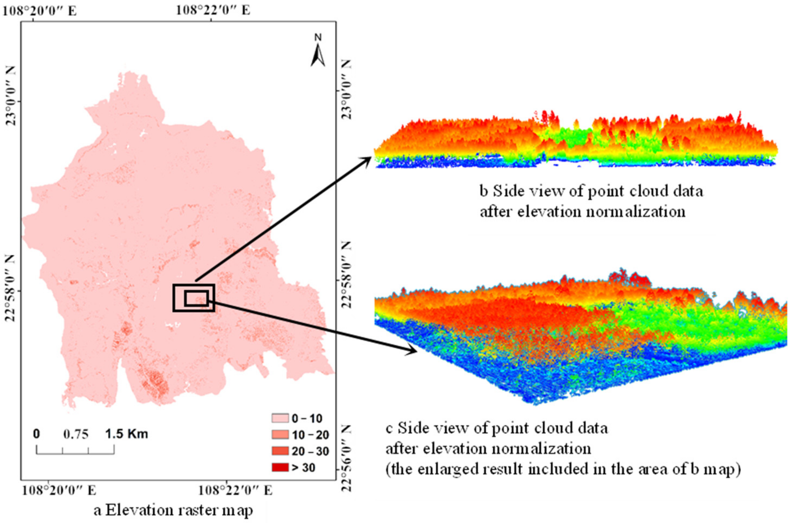
2.1.1. Study Area
2.1.2. Field Data
2.1.3. ALS Data
2.1.4. ALS Data Processing
2.2. Methods
2.2.1. Feature Variables Extraction
2.2.2. Feature Variables Selection
2.2.3. Regression Modeling of AGB
2.2.4. Accuracy Evaluation
3. Results
3.1. Feature Selection
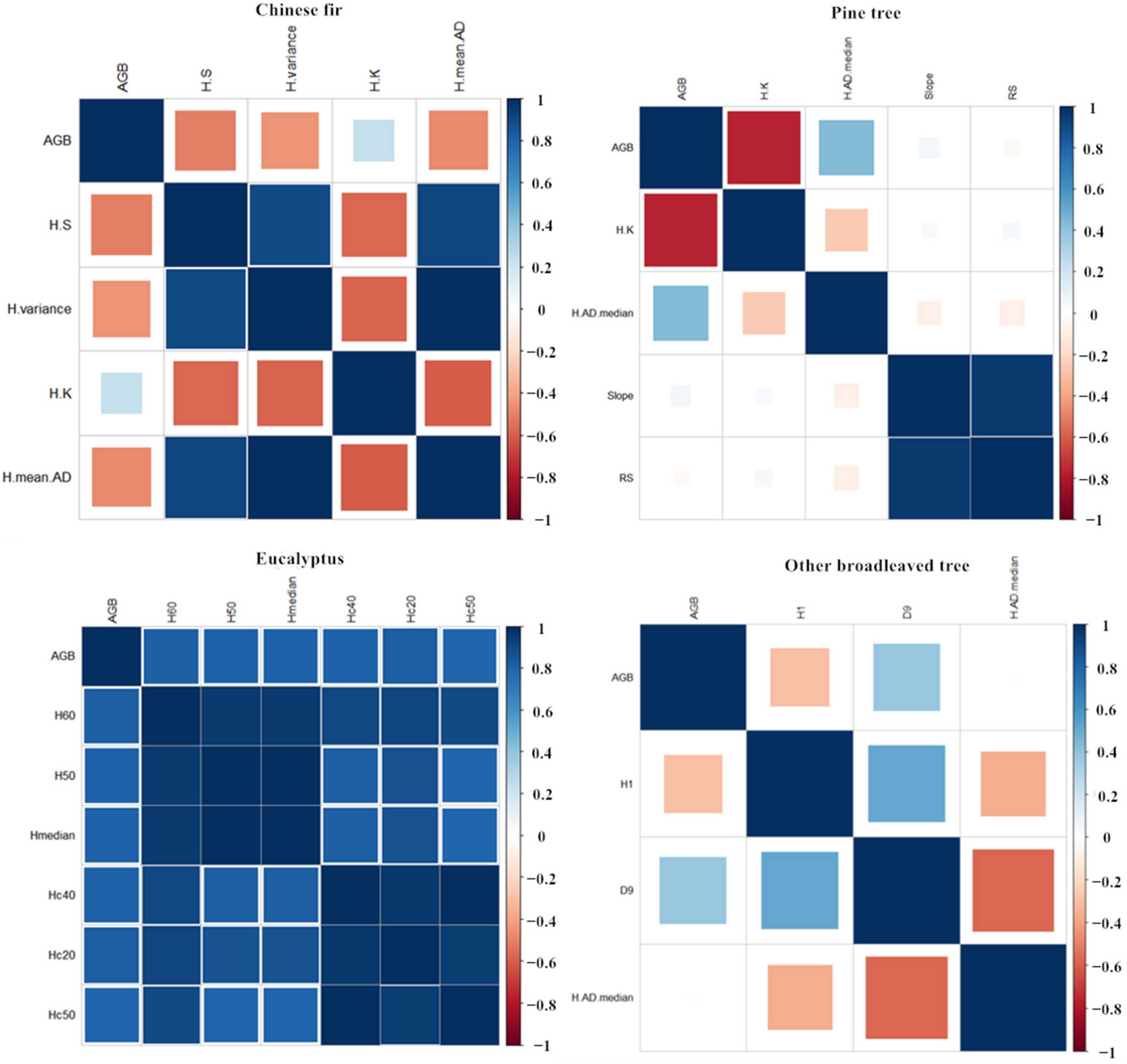
3.2. Correlation Analysis
3.3. AGB Estimation Models
3.4. Accuracy Evaluation
3.5. Testing Accuracy
3.6. Forest Above-Ground Biomass Mapping
4. Discussion
- (a)
- There are differences in the optimal feature variables of different tree species. Compared with most previous studies, most of the point cloud feature variables related to aboveground biomass are height features [19,21]. In this study, the optimal features of pine trees include terrain features, and for other broadleaved trees they include point cloud density features. It also shows that the optimal features of different tree species are different, and the height feature alone cannot depict the aboveground biomass content of all tree species. Under complex terrain conditions, terrain variables should be added, and for broadleaved trees, point cloud density features must be considered as modeling variables.
- (b)
- It is a great advantage to distinguish tree species for estimating regional forest aboveground biomass. Compared with the forest AGB estimation in the same area, Zhang LQ [53] used Landsat TM data to estimate the forest AGB in the Gaofeng forest farm and constructed a multivariate linear equation. The accuracy was only 0.571. Compared with the forest AGB estimation using LiDAR point cloud data, Fu t et al. [54] used airborne LiDAR data to estimate forest AGB in Central Yunnan Province and distinguished three forest types, including coniferous forest, broadleaved forest and mixed forest. The results showed that the AGB estimation accuracy of coniferous forest was 0.68, and that of broadleaved forests was 0.43. From the above comparisons, it can be concluded that it is necessary to distinguish tree species for estimating regional forest AGB.
- (c)
- The accuracy of tree species classification and distribution will affect the accuracy of regional forest AGB distribution. The regional data used in this study are the sub-compartment data of forest resources inventory, and the statistical unit is the sub-compartment. The information of tree species in the sub-compartment pertains to the dominant tree species, not the exact distribution of each tree species. Therefore, how to improve the accuracy of tree species classification and map to fine patches rather than the sub-compartment is the main direction of follow-up research.
- (d)
- In this study, only forest AGB in a specific area was estimated by tree species. Whether these models can be applied in other regions of same tree species has not been compared and analyzed, which will be the focus of further research.
5. Conclusions
- (a)
- 63 features of point cloud data were extracted, including tree canopy feature, terrain features, point cloud vertical distribution and point cloud density features. The top features are mostly related to the height. Since pine trees are affected by the actual sample plot environment, the tree structure is also related to the terrain factors. Other broadleaved trees have different tree species composition, so the tree shape is also related to the point cloud density features. It can be concluded that the AGB determinants of different tree species are different, which are affected by various external conditions such as environment, tree species composition and forest age.
- (b)
- Considering the training accuracy, testing accuracy and complexity of stepwise regression, ridge regression, principal component regression and nonlinear regression models, the accuracy of the stepwise regression model was higher than that of nonlinear model, and the model was the simplest. Therefore, the stepwise regression method could be used to estimate forest AGB. The estimation accuracy of pine tree and eucalyptus AGB was more than 0.7, while Chinese fir and other broadleaved tree AGB was low, and that of Chinese fir was only 0.19. In conclusion, the AGB models of pine tree and eucalyptus can be used in practice, and the AGB models of Chinese fir and other broadleaved trees need to be optimized and verified.
Author Contributions
Funding
Data Availability Statement
Acknowledgments
Conflicts of Interest
References
- Shen, Y.; Cheng, R.; Xiao, W.; Yang, S.; Guo, Y.; Wang, N.; Zeng, L.; Wang, X. Labile organic carbon pools and enzyme activities of Pinus massoniana plantation soil as affected by understory vegetation removal and thinning. Sci. Rep. 2018, 8, 573. [Google Scholar] [CrossRef] [PubMed] [Green Version]
- Sun, P.; Jia, H.; Zhang, Y.; Li, J.; Lu, M.; Hu, J. Deciphering Genetic Architecture of Adventitious Root and Related Shoot Traits in Populus Using QTL Mapping and RNA-Seq Data. Int. J. Mol. Sci. 2019, 20, 6114. [Google Scholar] [CrossRef] [PubMed] [Green Version]
- Schwaab, J.; Davin, E.L.; Bebi, P.; Duguay-Tetzlaff, A.; Waser, L.T.; Haeni, M.; Meier, R. Increasing the broad-leaved tree fraction in European forests mitigates hot temperature extremes. Sci. Rep. 2020, 10, 1–9. [Google Scholar] [CrossRef] [PubMed]
- Vorster, A.G.; Evangelista, P.H.; Stovall, A.E.L.; Ex, S. Variability and uncertainty in forest biomass estimates from the tree to landscape scale: The role of allometric equations. Carbon Balance Manag. 2020, 15, 1–20. [Google Scholar] [CrossRef]
- Beaudoin, G.; Rafanoharana, S.; Boissière, M.; Wijaya, A.; Wardhana, W. Completing the Picture: Importance of Considering Participatory Mapping for REDD+ Measurement, Reporting and Verification (MRV). PLoS ONE 2016, 11, e0166592. [Google Scholar] [CrossRef] [Green Version]
- Sarker, L.R.; Nichol, J.E. Improved forest biomass estimates using ALOS AVNIR-2 texture indices. Remote Sens. Environ. 2011, 115, 968–977. [Google Scholar] [CrossRef]
- Lay, U.S.; Pradhan, B.; Yusoff, Z.B.M.; Bin Abdallah, A.F.; Aryal, J.; Park, H.-J. Data Mining and Statistical Approaches in Debris-Flow Susceptibility Modelling Using Airborne LiDAR Data. Sensors 2019, 19, 3451. [Google Scholar] [CrossRef] [Green Version]
- Bouvier, M.; Durrieu, S.; Fournier, R.A.; Renaud, J.-P. Generalizing predictive models of forest inventory attributes using an area-based approach with airborne LiDAR data. Remote Sens. Environ. 2015, 156, 322–334. [Google Scholar] [CrossRef]
- Dash, J.P.; Watt, M.S.; Bhandari, S.; Watt, P. Characterising forest structure using combinations of airborne laser scanning data, RapidEye satellite imagery and environmental variables. Forests 2015, 89, 159–169. [Google Scholar] [CrossRef] [Green Version]
- Che, E.; Jung, J.; Olsen, M.J. Object Recognition, Segmentation, and Classification of Mobile Laser Scanning Point Clouds: A State of the Art Review. Sensors 2019, 19, 810. [Google Scholar] [CrossRef] [Green Version]
- Zhao, K.; Popescu, S.; Nelson, R. Lidar remote sensing of forest biomass: A scale-invariant estimation approach using airborne lasers. Remote Sens. Environ. 2009, 113, 182–196. [Google Scholar] [CrossRef]
- Gleason, C.J.; Im, J. Forest biomass estimation from airborne LiDAR data using machine learning approaches. Remote Sens. Environ. 2012, 125, 80–91. [Google Scholar] [CrossRef]
- Kronseder, K.; Ballhorn, U.; Böhm, V.; Siegert, F. Above ground biomass estimation across forest types at different degradation levels in Central Kalimantan using LiDAR data. Int. J. Appl. Earth Obs. Geoinf. 2012, 18, 37–48. [Google Scholar] [CrossRef]
- Fassnacht, F.E.; Latifi, H.; Hartig, F. Using synthetic data to evaluate the benefits of large field plots for forest biomass estimation with LiDAR. Remote Sens. Environ. 2018, 213, 115–128. [Google Scholar] [CrossRef]
- Cao, L.; Coops, N.C.; Sun, Y.; Ruan, H.; Wang, G.; Dai, J.; She, G. Estimating canopy structure and biomass in bamboo forests using airborne LiDAR data. ISPRS J. Photogramm. Remote Sens. 2019, 148, 114–129. [Google Scholar] [CrossRef]
- Zolkos, S.; Goetz, S.; Dubayah, R. A meta-analysis of terrestrial aboveground biomass estimation using lidar remote sensing. Remote Sens. Environ. 2013, 128, 289–298. [Google Scholar] [CrossRef]
- Takagi, K.; Yone, Y.; Takahashi, H.; Sakai, R.; Hojyo, H.; Kamiura, T.; Nomura, M.; Liang, N.; Fukazawa, T.; Miya, H.; et al. Forest biomass and volume estimation using airborne LiDAR in a cool-temperate forest of northern Hokkaido, Japan. Ecol. Inform. 2015, 26, 54–60. [Google Scholar] [CrossRef]
- Stovall, A.E.; Vorster, A.G.; Anderson, R.S.; Evangelista, P.H.; Shugart, H.H. Non-destructive aboveground biomass estimation of coniferous trees using terrestrial LiDAR. Remote Sens. Environ. 2017, 200, 31–42. [Google Scholar] [CrossRef]
- He, Q.; Chen, E.; An, R.; Li, Y. Above-Ground Biomass and Biomass Components Estimation Using LiDAR Data in a Coniferous Forest. Forests 2013, 4, 984–1002. [Google Scholar] [CrossRef] [Green Version]
- Shao, G.; Shao, G.; Gallion, J.; Saunders, M.R.; Frankenberger, J.R.; Fei, S. Improving Lidar-based aboveground biomass estimation of temperate hardwood forests with varying site productivity. Remote Sens. Environ. 2018, 204, 872–882. [Google Scholar] [CrossRef]
- Lu, J.; Wang, H.; Qin, S.; Cao, L.; Pu, R.; Li, G.; Sun, J. Estimation of aboveground biomass of Robinia pseudoacacia forest in the Yellow River Delta based on UAV and Backpack LiDAR point clouds. Int. J. Appl. Earth Obs. Geoinf. 2020, 86, 102014. [Google Scholar] [CrossRef]
- Salum, R.B.; Souza-Filho, P.W.M.; Simard, M.; Silva, C.A.; Fernandes, M.E.; Cougo, M.F.; Nascimento, W.D.; Rogers, K. Improving mangrove above-ground biomass estimates using LiDAR. Estuarine Coast. Shelf Sci. 2020, 236, 106585. [Google Scholar] [CrossRef]
- Yuanguang, W. Study on biomass and distribution of Cunninghamia lanceolata Plantation in Guangxi. J. Guangxi Agric. Univ. 1995, 14, 55–64. [Google Scholar]
- Yuanguang, W. Study on biomass and productivity of Eucalyptus urophylla plantation. J. Trop. Subtrop. Bot. 2000, 8, 123–127. [Google Scholar]
- Dou, L.; Deng, Q.; Li, M.; Wang, W. Biomass and distribution characteristics of Pinus massoniana plantations with different ages in Eastern Guangxi. Acta Bot. Boreali-Occident. Sin. 2013, 33, 394–400. [Google Scholar]
- Luo, Y.; Chen, C.G.; Zhu, J.F. A Handbook of Biomass Models for Major Forest Trees in China; China Forestry Publishing House: Beijing, China, 2015. [Google Scholar]
- Smigiel, E.; Alby, E.; Grussenmeyer, P. TLS data denoising by range image processing. Photogramm. Rec. 2011, 26, 171–189. [Google Scholar] [CrossRef]
- Qing, S.; Tao, X.; Tatsuo, Y.; Nan, S.; Hang, Z. Classified denoising method for laser point cloud data of stored grain bulk surface based on discrete wavelet threshold. Int. J. Agric. Biol. Eng. 2016, 9, 123–131. [Google Scholar]
- Gorgens, E.B.; Valbuena, R.; Rodriguez, L.C.E. A Method for Optimizing Height Threshold When Computing Airborne Laser Scanning Metrics. Photogramm. Eng. Remote Sens. 2017, 83, 343–350. [Google Scholar] [CrossRef]
- Lin, X.; Zhang, J. Segmentation-Based Filtering of Airborne LiDAR Point Clouds by Progressive Densification of Terrain Segments. Remote Sens. 2014, 6, 1294–1326. [Google Scholar] [CrossRef] [Green Version]
- Quan, Y.; Song, J.; Guo, X.; Miao, Q.; Yang, Y. Filtering LiDAR data based on adjacent triangle of triangulated irregular network. Multimed. Tools Appl. 2016, 76, 11051–11063. [Google Scholar] [CrossRef]
- Liu, H.; Wu, C. Developing a Scene-Based Triangulated Irregular Network (TIN) Technique for Individual Tree Crown Reconstruction with LiDAR Data. Forests 2019, 11, 28. [Google Scholar] [CrossRef] [Green Version]
- Yang, X. Cover: Use of LIDAR elevation data to construct a high-resolution digital terrain model for an estuarine marsh area. Int. J. Remote Sens. 2005, 26, 5163–5166. [Google Scholar] [CrossRef]
- Polat, N.; Uysal, M.; Toprak, A. An investigation of DEM generation process based on LiDAR data filtering, decimation, and interpolation methods for an urban area. Measurement 2015, 75, 50–56. [Google Scholar] [CrossRef]
- Ma, Q.; Su, Y.; Guo, Q. Comparison of Canopy Cover Estimations From Airborne LiDAR, Aerial Imagery, and Satellite Imagery. IEEE J. Sel. Top. Appl. Earth Obs. Remote Sens. 2017, 10, 4225–4236. [Google Scholar] [CrossRef]
- Richardson, J.J.; Moskal, L.M.; Kim, S.-H. Modeling approaches to estimate effective leaf area index from aerial discrete-return LIDAR. Agric. For. Meteorol. 2009, 149, 1152–1160. [Google Scholar] [CrossRef]
- Cao, D.-S.; Liang, Y.-Z.; Xu, Q.-S.; Zhang, L.-X.; Hu, Q.-N.; Li, H.-D. Feature importance sampling-based adaptive random forest as a useful tool to screen underlying lead compounds. J. Chemom. 2011, 25, 201–207. [Google Scholar] [CrossRef]
- Wang, G.; Fu, G.; Corcoran, C. A forest-based feature screening approach for large-scale genome data with complex structures. BMC Genet. 2015, 16, 1–11. [Google Scholar] [CrossRef] [Green Version]
- Huang, C.; Townshend, J.R.G. A stepwise regression tree for nonlinear approximation: Applications to estimating subpixel land cover. Int. J. Remote Sens. 2003, 24, 75–90. [Google Scholar] [CrossRef]
- Wang, M.; Wright, J.; Brownlee, A.; Buswell, R. A comparison of approaches to stepwise regression on variables sensitivities in building simulation and analysis. Energy Build. 2016, 127, 313–326. [Google Scholar] [CrossRef] [Green Version]
- Hoerl, A.E.; Kennard, R.W. Ridge regression: Biased estimation for nonorthogonal problems. Technometrics 1970, 12, 55–67. [Google Scholar] [CrossRef]
- Park, M.; Yang, M. Ridge Regression Estimation for Survey Samples. Commun. Stat. Theory Methods 2008, 37, 532–543. [Google Scholar] [CrossRef]
- Kaçıranlar, S.; Sakallıoğlu, S.; Özkale, M.R.; Güler, H. More on the restricted ridge regression estimation. J. Stat. Comput. Simul. 2011, 81, 1433–1448. [Google Scholar] [CrossRef]
- Liu, X.-Q.; Gao, F.; Xu, J.-W. Linearized Restricted Ridge Regression Estimator in Linear Regression. Commun. Stat. Theory Methods 2012, 41, 4503–4514. [Google Scholar] [CrossRef]
- Massy, W.F. Principal Components Regression in Exploratory Statistical Research. J. Am. Stat. Assoc. 1965, 60, 234. [Google Scholar] [CrossRef]
- Ieong, I.I.; Lou, I.; Ung, W.K.; Mok, K.M. Using principle component regression, artificial neural network, and hybrid models for predicting phytoplankton abundance in Macau storage reservoir. Environ. Modeling Assess. 2015, 20, 355–365. [Google Scholar] [CrossRef]
- Xiong, W.; Shi, X. Soft sensor modeling with a selective updating strategy for Gaussian process regression based on probabilistic principle component analysis. J. Frankl. Inst. 2018, 355, 5336–5349. [Google Scholar] [CrossRef]
- Zhang, W.; Lou, I.C.; Kong, Y.; Ung, W.K.; Mok, K.M. Eutrophication analyses and principle component regression for two subtropical storage reservoirs in Macau. Desalination Water Treat. 2013, 51, 7331–7340. [Google Scholar] [CrossRef]
- Tran, H.; Kim, J.; Kim, D.; Choi, M.; Choi, M. Impact of air pollution on cause-specific mortality in Korea: Results from Bayesian Model Averaging and Principle Component Regression approaches. Sci. Total Environ. 2018, 636, 1020–1031. [Google Scholar] [CrossRef]
- Farhadur Rahman, M.; Onoda, Y.; Kitajima, K. Forest canopy height variation in relation to topography and forest types in central Japan with LiDAR. For. Ecol. Manag. 2022, 503, 119792. [Google Scholar] [CrossRef]
- Knapp, N.; Fischer, R.; Cazcarra-Bes, V.; Huth, A. Structure metrics to generalize biomass estimation from lidar across forest types from different continents. Remote Sens. Environ. 2020, 237, 111597. [Google Scholar] [CrossRef]
- Jin, S.; Su, Y.; Song, S.; Xu, K.; Hu, T.; Yang, Q.; Wu, F.; Xu, G.; Ma, Q.; Guan, H.; et al. Non-destructive estimation of field maize biomass using terrestrial lidar: An evaluation from plot level to individual leaf level. Plant Methods 2020, 16, 1–19. [Google Scholar] [CrossRef]
- Zhang, L.Q. Research on Remote sensing Biomass Estimate of Eucalyptus Plantation; Guangxi University: Nanning, China, 2012. [Google Scholar]
- Fu, T.; Pang, Y.; Huang, Q.; Liu, Q.; Xu, G. Prediction of subtropical forest parameters using airborne laser scanner. J. Remote Sens. 2011, 15, 1092–1104. [Google Scholar]


| Plot No. | Species | Plot Size (m2) | Inventoried Trees (All Trees/Sample Trees) | Forest Type | Training/Testing Dataset | Number of Plots | Diameter at Breast Height (DBH cm) | Tree Height (m) | Stem Density (n·ha−1) | AGB (t·ha−1) |
|---|---|---|---|---|---|---|---|---|---|---|
| 1–27 | Chinese fir | 20 × 20 | All trees | Middle | Training | 2 | 17.9 ± 11.9 | 13 ± 6.5 | 1200 ± 0 | 92.8 ± 5.5 |
| Testing | 4 | 22.8 ± 18.1 | 15.6 ± 10 | 900 ± 300 | 87.8 ± 2.7 | |||||
| 25 × 25 | All trees | Middle | Training | 6 | 28.1 ± 20.8 | 19.5 ± 12.6 | 624 ± 160 | 83.8 ± 24 | ||
| Testing | 4 | 22.1 ± 8.7 | 16.6 ± 4.8 | 656 ± 96 | 82.7 ± 2.8 | |||||
| 30 × 30 | Sample trees | Middle | Training | 9 | 15.5 ± 4.4 | 13.6 ± 2.6 | 2272 ± 1461 | 82.7 ± 22.2 | ||
| Testing | 2 | 14.6 ± 1 | 13.4 ± 1.5 | 1744 ± 389 | 88.5 ± 2.5 | |||||
| 28–42 | Pine tree | 30 × 30 | Sample trees | Middle | Training/ testing | 6 | 22 ± 3.9 | 16.8 ± 1.5 | 1211 ± 667 | 139.7 ± 36.1 |
| Young | Training/ testing | 9 | 15.2 ± 2.5 | 9.4 ± 3.3 | 1333 ± 345 | 126.4 ± 73.2 | ||||
| 43–77 | Eucalyptus | 20 × 20 | All trees | Middle | Training | 1 | 17.4 ± 8.4 | 21.3 ± 4.4 | 1300 | 185.7 |
| Testing | 2 | 23.1 ± 9.4 | 24.5 ± 10 | 937 ± 163 | 301 ± 37.8 | |||||
| Young | Training | 8 | 10.3 ± 7.3 | 14.2 ± 8.6 | 1887 ± 838 | 67.3 ± 54.2 | ||||
| Testing | 7 | 12.3 ± 7.1 | 11.3 ± 10 | 1537 ± 188 | 58 ± 33.5 | |||||
| 25 × 25 | All trees | Middle | Training | 7 | 17 ± 11.5 | 20.8 ± 11.8 | 1232 ± 656 | 204.2 ± 91 | ||
| Young | Training | 3 | 12.1 ± 7.7 | 13.1 ± 6.3 | 1608 ± 616 | 89.5 ± 34 | ||||
| 30 × 30 | Sample trees | Young | Training | 4 | 10.4 ± 0.8 | 15.2 ± 1.9 | 1855 ± 423 | 85.1 ± 32.8 | ||
| Testing | 3 | 10.1 ± 2.4 | 14.5 ± 2.7 | 2177 ± 467 | 82.8 ± 33.3 | |||||
| 78–98 | Other broadleaved trees | 25 × 25 | All trees | Middle | Training | 3 | 18.7 ± 14.4 | 13.1 ± 9 | 1192 ± 312 | 209.6 ± 81.2 |
| Testing | 3 | 28.5 ± 21.5 | 15.8 ± 9.8 | 944 ± 240 | 227.7 ± 21.3 | |||||
| 30 × 30 | Sample trees | Middle | Training | 8 | 14.5 ± 5.3 | 13.9 ± 5.6 | 1233 ± 478 | 164.5 ± 112.4 | ||
| Testing | 7 | 18.1 ± 5 | 14.7 ± 4.1 | 1372 ± 806 | 172.3 ± 31.8 |
| Parameters | Value |
|---|---|
| Wavelength (nm) | 1550 |
| Divergence angle (mrad) | 0.5 |
| Step length (cm) | 45 |
| Pulse repetition rate (KHz) | 360 |
| Scanning rate (Hz) | 112 |
| Width (m) | 1040 |
| Flight altitude (m) | 900 |
| Flight speed (m/s) | 55 |
| Side overlap | 65% |
| Average point spacing (m) | 0.45 × 0.45 |
| Category | Search Radius (m) | Height Difference (m) | Minimum Height (m) | Maximum Height (m) | Maximum Terrain Slope Angle (°) | Iteration Angle (°) | Iteration Distance (m) |
|---|---|---|---|---|---|---|---|
| High point | 3 | >5 | |||||
| Low point | 3 | <0.5 | |||||
| Ground point | 88 | 8 | 1.5 | ||||
| Surface vegetation point | 0 | 0.3 | |||||
| Forest point | 0.3 | 50 |
| Feature Number | Feature | Meaning | Abbreviation |
|---|---|---|---|
| 1 | Canopy density [35] | The ratio of vegetation points to total points in a unit grid | C.density |
| 2 | Spacing rate [36] | The ratio of ground points to total points in a unit grid | Gap |
| 3 | Leaf area index [36] | Half of the leaf surface in a unit grid | LAI |
| 4 | Canopy fluctuation rate [35] | H.clr |
| Feature Number | Feature | Meaning | Abbreviation |
|---|---|---|---|
| 5 | Roughness | The ratio of the surface area to its projected area on a horizontal plane | RS |
| 6 | Slope | The steepness of terrain surface based on the DEM | Slope |
| 7 | Aspect | The projection direction of slope normal line on a horizontal plane based on the DEM | Aspect |
| 8 | Mountain shadow | The brightness of each pixel based on the DEM | Shadow |
| Feature Number | Feature | Meaning | Abbreviation |
|---|---|---|---|
| 9 | Mean absolute deviation | H.mean.AD | |
| 10 | Median absolute deviation | H.AD.median | |
| 11–25 | Cumulative Height Percentile | The height sum of X% points in a unit grid | Hc1-Hc99 |
| 26 | Inter-quartile Range of Cumulative Height | Difference of Hc75 and Hc25 | Hc.S |
| 27–41 | Height Percentile | The height of X% points in a unit grid | H1-H99 |
| 42 | Inter-quartile Range | Difference of H75 and H25 | H.S |
| 43 | Kurtosis | Kurtosis of all point height in a unit grid | H.K |
| 44 | Variation Coefficient | H.cv | |
| 45 | Mean Quadratic Power | H.sq.mean | |
| 46 | Mean Cubic Power | H.c.mean | |
| 47 | Maximum | Max height of all points in a unit grid | Hmax |
| 48 | Minimum | Min height of all points in a unit grid | Hmin |
| 49 | Mean | Mean height of all points in a unit grid | Hmean |
| 50 | Median | Median height of all points in a unit grid | Hmedian |
| 51 | Skewness | H.skewness | |
| 52 | Standard Deviation | Std height of all points in a unit grid | H.std |
| 53 | Variance | Var height of all points in a unit grid | H.variance |
| Feature Number | Feature | Meaning | Abbreviation |
|---|---|---|---|
| 54–63 | Point density in each horizontal layer | The point cloud was sliced to ten horizontal layers with the same heights. D1 to D10 corresponded to the point density from the lowest layer to the highest (D1 is the lowest layer) | D1–D10 |
| Tree Species | Method | Model | Training Accuracy R2 |
|---|---|---|---|
| Chinese fir | SR | Y = 108.5 − 4.7 × H.mean.AD | 0.23 |
| Ridge | Y = 101.9 − 0.7 × H.S − 0.1 × H.variance − 0.01 × H.K − 1.3 × H.mean.AD | 0.25 | |
| PCR | Y = 109.5 − 0.8 × H.S − 0.2 × H.variance − 0.6 × H.K − 1.8 × H.mean.AD | 0.24 | |
| Non | Y = 1048.5 + 5.4 × H.S2 − 3.0 × H.variance2 + 5.5 × H.K2 − 284.5 × H.mean.AD2 + 24.9 × H.S × H.variance − 92.4 × H.S × H.K − 170.6 × H.S × H.mean.AD + 51.6 × H.variance × H.K + 62.5 × H.variance × H.mean.AD − 262.2 × H.K × H.mean.AD − 19.9 × H.S × H.variance × H.K − 1.5 × H.S × H.variance × H.mean.AD + 137.1 × H.S × H.K × H.mean.AD − 5.8 × H.variance × H.K × H.mean.AD + 1.1 × H.S × H.variance × H.K × H.mean.AD | 0.9 | |
| Pine tree | SR | Y = 120.7 − 9.5 × H.K + 6.6 × H.AD.median + 4.7 × Slope − 32.5 × RS | 0.72 |
| Ridge | Y = 135.0 − 8.4 × H.K + 6.2 × H.AD.median + 1.3 × Slope − 7.5 × RS | 0.69 | |
| PCR | Y = 116.1 − 6.7 × H.K + 12.2 × H.AD.median + 0.2 × Slope + 1.5 × RS | 0.58 | |
| Non | Y = − 12790 − 20.7 × H.K2 − 420.9 × H.AD.median2 + 78.8 × Slope2 + 3019.7 × RS2 + 3502.1 × H.K × H.AD.median − 240.0 × H.K × Slope + 4364.5 × H.K × RS − 487.3 × H.AD.median × Slope + 9880.1 × H.AD.median × RS − 929.8 × Slope × RS + 80.4 × H.K × H.AD.median × Slope − 4487.1 × H.K × H.AD.median × RS − 76.6 × H.K × Slope × RS − 169.6 × H.AD.median × Slope × RS + 93.1 × H.K × H.AD.median × Slope × RS | 0.98 | |
| Eucalyptus | SR | Y = − 28.6 + 3.6 × H50 + 5.0 × Hc40 | 0.72 |
| Ridge | Y = − 26.6 + 0.4 × H60 + 1.4 × H50 + 1.4 × Hmedian + 1.7 × Hc40 + 2.3 × Hc20 + 1.3 × Hc50 | 0.72 | |
| PCR | Y = − 27.2 + 1.2 × H60 + 1.2 × H50 + 1.2 × Hmedian + 1.6 × Hc40 + 1.7 × Hc20 + 1.6 × Hc50 | 0.71 | |
| Non | Y = 2914 − 178.3 × H60 −0.02 − 3066.9 × Hc50 −0.05 | 0.56 | |
| Other broadleaved trees | SR | Y = 114.6 − 11.4 × H1 + 302.3 × D9 | 0.48 |
| Ridge | Y = 96.7 − 8.4 × H1 + 264.9 × D9 + 7.7 × H.AD.median | 0.52 | |
| PCR | Y = 201.2 − 5.3 × H1 + 28.9 × D9 − 14.1 × H.AD.median | 0.12 | |
| Non | Y = 142.4 + 16.7 × H12 + 583.8 × D92 + 1.6 × H.AD.median2 − 1989.8 × H1 × D9 − 99.9 × H1 × H.AD.median − 18.5 × D9 × H.AD.median + 1227.6 × H1 × D9 × H.AD.median | 0.79 |
| Tree Species | Method | Maximum | Minimum | Average | Proportion Above 0.8 |
|---|---|---|---|---|---|
| Chinese fir | SR | 0.997 | 0.895 | 0.961 | 1 |
| Ridge | 0.997 | 0.900 | 0.952 | 1 | |
| PCR | 0.997 | 0.880 | 0.953 | 1 | |
| Non | 0.834 | 0.128 | 0.567 | 0.1 | |
| Pine tree | SR | 0.991 | 0.286 | 0.842 | 0.73 |
| Ridge | 0.998 | 0.144 | 0.835 | 0.8 | |
| PCR | 0.995 | 0.303 | 0.845 | 0.73 | |
| Non | 0.801 | −39.343 | −2.886 | 0.07 | |
| Eucalyptus | SR | 0.998 | −0.289 | 0.780 | 0.67 |
| Ridge | 0.981 | −0.267 | 0.771 | 0.67 | |
| PCR | 1.267 | −0.273 | 0.876 | 0.75 | |
| Non | 0.967 | −5.085 | 0.163 | 0.17 | |
| Other broadleaved trees | SR | 0.962 | 0.553 | 0.839 | 0.8 |
| Ridge | 0.980 | 0.580 | 0.823 | 0.8 | |
| PCR | 0.985 | 0.542 | 0.846 | 0.8 | |
| Non | 0.996 | 0.603 | 0.859 | 0.8 |
| Tree Species | Method | Testing Accuracy R2 | RMSE (t/hm2) | MAE (t/hm2) |
|---|---|---|---|---|
| Chinese fir | SR | 0.19 | 4.25 | 3.40 |
| Ridge | 0.07 | 4.78 | 4.11 | |
| PCR | 0.11 | 5.02 | 4.10 | |
| Non | 0.09 | 42.71 | 37.44 | |
| Pine tree | SR | 0.76 | 21.18 | 17.28 |
| Ridge | 0.73 | 23.19 | 18.56 | |
| PCR | 0.64 | 25.69 | 17.90 | |
| Non | 0.13 | 1118.00 | 303.96 | |
| Eucalyptus | SR | 0.71 | 50.75 | 25.48 |
| Ridge | 0.68 | 53.33 | 27.84 | |
| PCR | 0.69 | 52.41 | 27.83 | |
| Non | 0.11 | 168.79 | 79.94 | |
| Other broadleaved trees | SR | 0.40 | 46.28 | 33.80 |
| Ridge | 0.51 | 46.78 | 36.05 | |
| PCR | 0.01 | 47.24 | 33.27 | |
| Non | 0.32 | 44.85 | 31.62 |
| Tree Species | The Number of Sub-Compartment | The Area of Sub-Compartment (ha) | AGB of Sub-Compartment (t·ha−1) |
|---|---|---|---|
| Chinese fir | 80 | 8.495 ± 8.475 | 89.24 ± 14.89 |
| Pine tree | 63 | 7.835 ± 7.655 | 146.11 ± 54.83 |
| Eucalyptus | 391 | 8.595 ± 8.575 | 81.17 ± 68.82 |
| Other broadleaved trees | 234 | 6.795 ± 6.745 | 149.795 ± 125.925 |
Publisher’s Note: MDPI stays neutral with regard to jurisdictional claims in published maps and institutional affiliations. |
© 2021 by the authors. Licensee MDPI, Basel, Switzerland. This article is an open access article distributed under the terms and conditions of the Creative Commons Attribution (CC BY) license (https://creativecommons.org/licenses/by/4.0/).
Share and Cite
Gao, L.; Zhang, X. Above-Ground Biomass Estimation of Plantation with Complex Forest Stand Structure Using Multiple Features from Airborne Laser Scanning Point Cloud Data. Forests 2021, 12, 1713. https://doi.org/10.3390/f12121713
Gao L, Zhang X. Above-Ground Biomass Estimation of Plantation with Complex Forest Stand Structure Using Multiple Features from Airborne Laser Scanning Point Cloud Data. Forests. 2021; 12(12):1713. https://doi.org/10.3390/f12121713
Chicago/Turabian StyleGao, Linghan, and Xiaoli Zhang. 2021. "Above-Ground Biomass Estimation of Plantation with Complex Forest Stand Structure Using Multiple Features from Airborne Laser Scanning Point Cloud Data" Forests 12, no. 12: 1713. https://doi.org/10.3390/f12121713