Comparison of Canopy Closure Estimation of Plantations Using Parametric, Semi-Parametric, and Non-Parametric Models Based on GF-1 Remote Sensing Images


Abstract
:1. Introduction
2. Materials and Methods
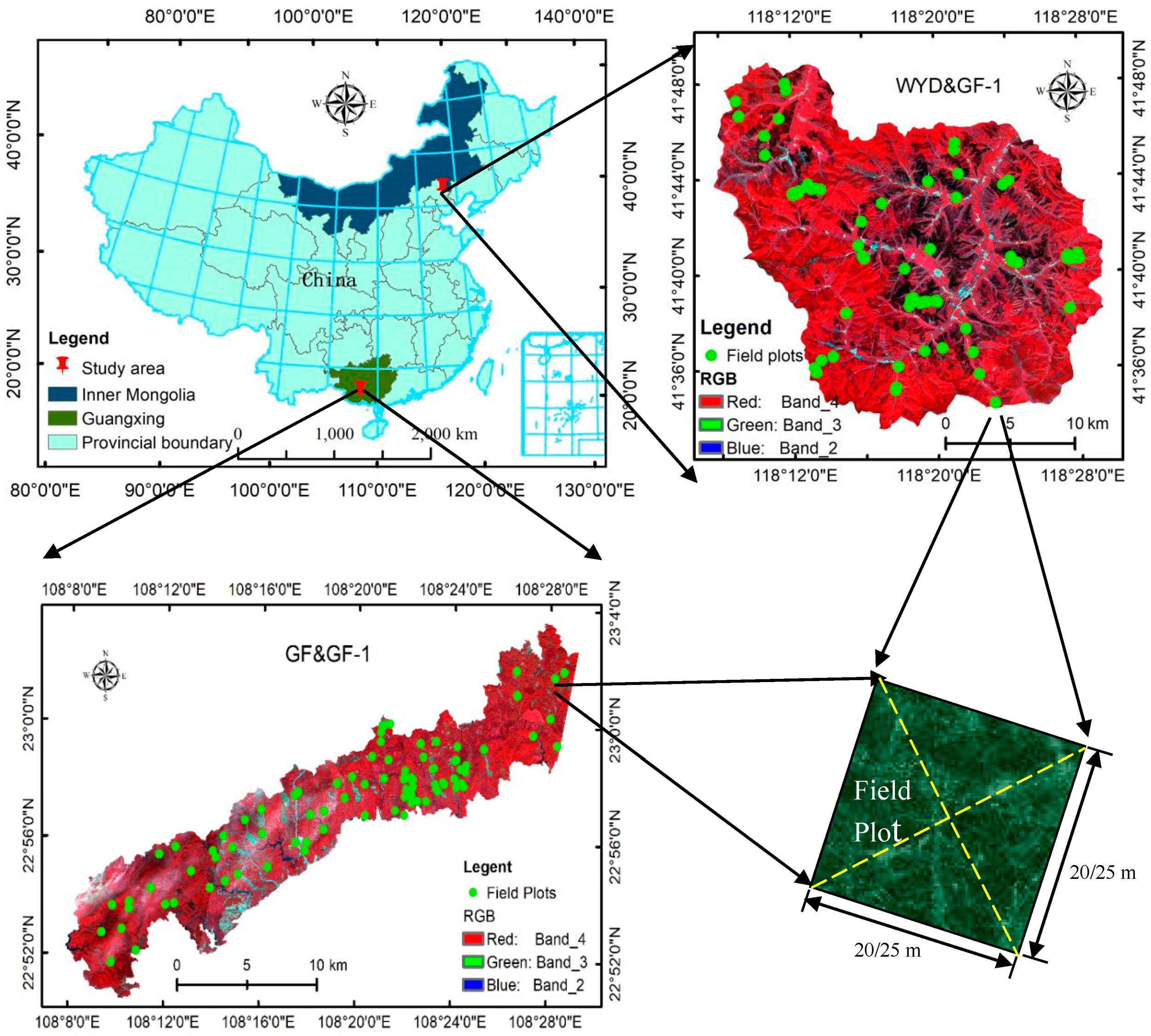
2.1. Study Area
2.2. Data
2.2.1. Remote Sensing Data
2.2.2. Field Data
2.3. Methods
2.3.1. Remote Sensing Variable Extraction
2.3.2. Canopy Closure Estimation Models
Multiple Linear Regression
Generalized Additive Model (GAM)
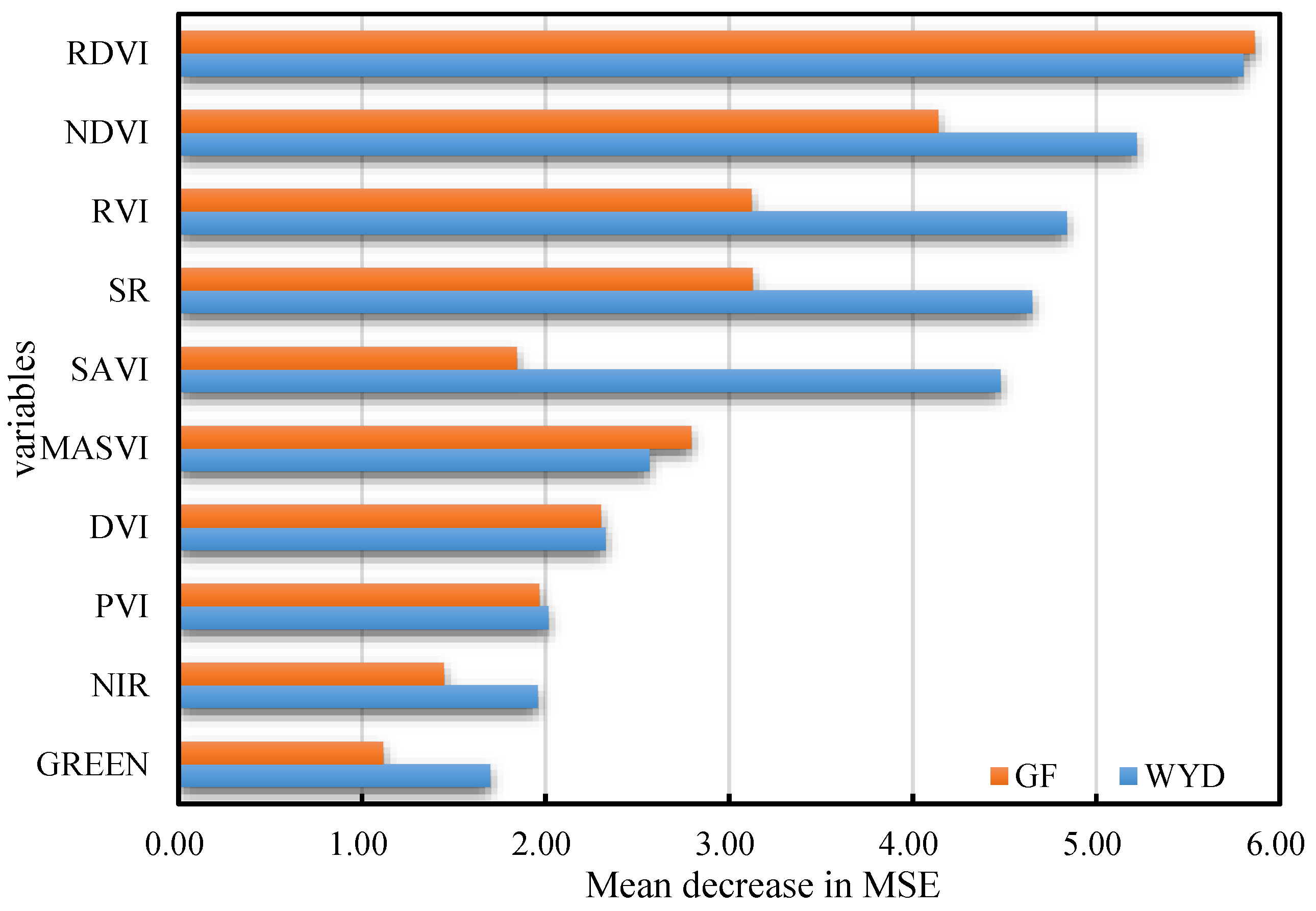
Random Forest
2.4. Model Inspection
3. Results
4. Discussion
5. Conclusions
Author Contributions
Funding
Acknowledgments
Conflicts of Interest
References
- Jennings, S.; Brown, N.; Sheil, D. Assessing forest canopies and understorey illumination: Canopy closure, canopy cover and other measures. Forestry 1999, 72, 59–74. [Google Scholar] [CrossRef]
- FAO. Global forest resources assessment 2005. In FAO Forestry Paper 147; FAO: Rome, Italy, 2006; p. 350. [Google Scholar]
- Chen, J.M.; Cihlar, J. Retrieving leaf area index of boreal conifer forests using Landsat TM images. Remote Sens. Environ. 1996, 55, 153–162. [Google Scholar] [CrossRef]
- Fassnacht, K.S.; Gower, S.T.; MacKenzie, M.D.; Nordheim, E.V.; Lillesand, T.M. Estimating the leaf area index of North Central Wisconsin forests using the landsat thematic mapper. Remote Sens. Environ. 1997, 61, 229–245. [Google Scholar] [CrossRef]
- Gobron, N.; Pinty, B.; Verstraete, M. Theoretical limits to the estimation of the leaf area index on the basis of visible and near-infrared remote sensing data. IEEE Trans. Geosci. Remote Sens. 1997, 35, 1438–1445. [Google Scholar] [CrossRef]
- Chen, J.M.; Leblanc, S.G.; Miller, J.R.; Freemantle, J.; Loechel, S.E.; Walthall, C.L.; Innanen, K.A.; White, H.P. Compact Airborne Spectrographic Imager (CASI) used for mapping biophysical parameters of boreal forests. J. Geophys. Res. Space Phys. 1999, 104, 27945–27958. [Google Scholar] [CrossRef]
- Hu, B.; Inannen, K.; Miller, J.R. Retrieval of Leaf Area Index and Canopy Closure from CASI Data over the BOREAS Flux Tower Sites. Remote Sens. Environ. 2000, 74, 255–274. [Google Scholar] [CrossRef]
- Fiala, A.C.; Garman, S.L.; Gray, A.N. Comparison of five canopy cover estimation techniques in the western Oregon Cascades. For. Ecol. Manag. 2006, 232, 188–197. [Google Scholar] [CrossRef]
- Halperin, J.; Lemay, V.; Coops, N.C.; Verchot, L.; Marshall, P.; Lochhead, K. Canopy cover estimation in miombo woodlands of Zambia: Comparison of Landsat 8 OLI versus RapidEye imagery using parametric, nonparametric, and semiparametric methods. Remote Sens. Environ. 2016, 179, 170–182. [Google Scholar] [CrossRef]
- Moeser, D.; Roubinek, J.; Schleppi, P.; Morsdorf, F.; Jonas, T. Canopy closure, LAI and radiation transfer from airborne LiDAR synthetic images. Agric. For. Meteorol. 2014, 197, 158–168. [Google Scholar] [CrossRef]
- Wallace, L.; Lucieer, A.; Malenovsky, Z.; Turner, D.; Vopěnka, P. Assessment of Forest Structure Using Two UAV Techniques: A Comparison of Airborne Laser Scanning and Structure from Motion (SfM) Point Clouds. Forests 2016, 7, 62. [Google Scholar] [CrossRef] [Green Version]
- Granholm, A.-H.; Lindgren, N.; Olofsson, K.; Nyström, M.; Allard, A.; Olsson, H. Estimating vertical canopy cover using dense image-based point cloud data in four vegetation types in southern Sweden. Int. J. Remote Sens. 2017, 38, 1–19. [Google Scholar] [CrossRef]
- Korhonen, L.; Korpela, I.; Heiskanen, J.; Maltamo, M. Airborne discrete-return LIDAR data in the estimation of vertical canopy cover, angular canopy closure and leaf area index. Remote Sens. Environ. 2011, 115, 1065–1080. [Google Scholar] [CrossRef]
- Lee, A.; Lucas, R. A LiDAR-derived canopy density model for tree stem and crown mapping in Australian forests. Remote Sens. Environ. 2007, 111, 493–518. [Google Scholar] [CrossRef]
- Naidoo, L.; Mathieu, R.; Main, R.; Kleynhans, W.; Wessels, K.; Asner, G.P.; LeBlon, B. Savannah woody structure modelling and mapping using multi-frequency (X-, C- and L-band) Synthetic Aperture Radar data. ISPRS J. Photogramm. Remote Sens. 2015, 105, 234–250. [Google Scholar] [CrossRef] [Green Version]
- Urbazaev, M.; Thiel, C.; Mathieu, R.; Naidoo, L.; Levick, S.R.; Smit, I.P.; Asner, G.P.; Schmullius, C. Assessment of the mapping of fractional woody cover in southern African savannas using multi-temporal and polarimetric ALOS PALSAR L-band images. Remote Sens. Environ. 2015, 166, 138–153. [Google Scholar] [CrossRef] [Green Version]
- Sinha, S.; Jeganathan, C.; Sharma, L.K.; Nathawat, M.S. A review of radar remote sensing for biomass estimation. Int. J. Environ. Sci. Technol. 2015, 12, 1779–1792. [Google Scholar] [CrossRef] [Green Version]
- E Kennedy, R.; Andréfouët, S.; Cohen, W.B.; Gómez, C.; Griffiths, P.; Hais, M.; Healey, S.P.; Helmer, E.H.; Hostert, P.; Lyons, M.B.; et al. Bringing an ecological view of change to Landsat-based remote sensing. Front. Ecol. Environ. 2014, 12, 339–346. [Google Scholar] [CrossRef]
- Pu, R. Wavelet transform applied to EO-1 hyperspectral data for forest LAI and crown closure mapping. Remote Sens. Environ. 2004, 91, 212–224. [Google Scholar] [CrossRef]
- Chopping, M.J.; Moisen, G.G.; Su, L.; Laliberte, A.; Rango, A.; Martonchik, J.V.; Peters, D.P. Large area mapping of southwestern forest crown cover, canopy height, and biomass using the NASA Multiangle Imaging Spectro-Radiometer. Remote Sens. Environ. 2008, 112, 2051–2063. [Google Scholar] [CrossRef] [Green Version]
- Morisette, J.T.; Jarnevich, C.S.; Ullah, A.; Cai, W.; Pedelty, J.A.; Gentle, J.E.; Stohlgren, T.J.; Schnase, J.L. A tamarisk habitat suitability map for the continental United States. Front. Ecol. Environ. 2006, 4, 11–17. [Google Scholar] [CrossRef] [Green Version]
- Ruefenacht, B. Comparison of Three Landsat TM Compositing Methods: A Case Study Using Modeled Tree Canopy Cover. Photogramm. Eng. Remote Sens. 2016, 82, 199–211. [Google Scholar] [CrossRef]
- Korhonen, L.; Saputra, D.H.; Packalen, P.; Rautiainen, M. Comparison of Sentinel-2 and Landsat 8 in the estimation of boreal forest canopy cover and leaf area index. Remote Sens. Environ. 2017, 195, 259–274. [Google Scholar] [CrossRef]
- Saputra, D.H.; Korhonen, L.; Hovi, A.; Rönnholm, P.; Rautiainen, M. The accuracy of large-area forest canopy cover estimation using Landsat in boreal region. Int. J. Appl. Earth Obs. Geoinf. 2016, 53, 118–127. [Google Scholar] [CrossRef]
- Sun, H.; Korhonen, K.; Hantula, J.; Kasanen, R.A.O. Variation in properties ofPhlebiopsis gigantearelated to biocontrol against infection byHeterobasidionspp. in Norway spruce stumps. For. Pathol. 2009, 39, 133–144. [Google Scholar] [CrossRef]
- Pu, R.; Xu, B.; Gong, P. Oakwood crown closure estimation by unmixing Landsat TM data. Int. J. Remote Sens. 2003, 24, 4422–4445. [Google Scholar] [CrossRef]
- Xu, B.; Gong, P.; Pu, R. Crown closure estimation of oak savannah in a dry season with Landsat TM imagery: Comparison of various indices through correlation analysis. Int. J. Remote Sens. 2003, 24, 1811–1822. [Google Scholar] [CrossRef]
- Hojas-Gascon, L.; Cerutti, P.O.; Eva, H.; Nasi, R.; Martius, C. Monitoring Deforestation and Forest Degradation in the Context of REDD+: Lessons from Tanzania; Center for International Forestry Research (CIFOR): Bogor, Indonesia, 2015; pp. 1–8. [Google Scholar]
- Zeng, Y.; Schaepman, M.E.; Wu, B.; de Bruin, S.; Clevers, J.G.P.W. Change detection of forest crown closure using an inverted geometric-optical model and scaling. Remote Sens. Environ. 2008, 112, 4261–4271. [Google Scholar] [CrossRef]
- Jacquemoud, S. Inversion of the PROSPECT + SAIL canopy reflectance model from AVIRIS equivalent spectra: Theoretical study. Remote Sens. Environ. 1993, 44, 281–292. [Google Scholar] [CrossRef]
- Wolter, P.T.; Townsend, P.A.; Sturtevant, B.R. Estimation of forest structural parameters using 5 and 10 meter SPOT-5 satellite data. Remote Sens. Environ. 2009, 113, 2019–2036. [Google Scholar] [CrossRef]
- Cardenas, J.-S.; Wang, L. Retrieval of subpixel Tamarix canopy cover from Landsat data along the Forgotten River using linear and nonlinear spectral mixture models. Remote Sens. Environ. 2010, 114, 1777–1790. [Google Scholar] [CrossRef]
- Ahmed, O.S.; Franklin, S.E.; Wulder, M.A.; White, J.C. Characterizing stand-level forest canopy cover and height using Landsat time series, samples of airborne LiDAR, and the Random Forest algorithm. ISPRS J. Photogramm. Remote Sens. 2015, 101, 89–101. [Google Scholar] [CrossRef]
- Marvin, D.C.; Asner, G.P.; Schnitzer, S.A. Liana canopy cover mapped throughout a tropical forest with high-fidelity imaging spectroscopy. Remote Sens. Environ. 2016, 176, 98–106. [Google Scholar] [CrossRef] [Green Version]
- Carreiras, J.M.B.; Pereira, J.M.C.; Pereira, J. Estimation of tree canopy cover in evergreen oak woodlands using remote sensing. For. Ecol. Manag. 2006, 223, 45–53. [Google Scholar] [CrossRef]
- Karlson, M.; Ostwald, M.; Reese, H.; Sanou, J.; Tankoano, B.; Mattsson, E. Mapping Tree Canopy Cover and Aboveground Biomass in Sudano-Sahelian Woodlands Using Landsat 8 and Random Forest. Remote Sens. 2015, 7, 10017–10041. [Google Scholar] [CrossRef] [Green Version]
- Smith, A.; Falkowski, M.J.; Hudak, A.T.; Evans, J.; Robinson, A.P.; Steele, C.M. A cross-comparison of field, spectral, and lidar estimates of forest canopy cover. Can. J. Remote Sens. 2009, 35, 447–459. [Google Scholar] [CrossRef]
- Remote Sensing Market Service Platform of the Chinese Academy of Sciences. Available online: http://www.rscloudmart.com (accessed on 30 May 2018).
- China Resources Satellite Application Center. Available online: http://www.cresda.com/CN/ (accessed on 30 May 2018).
- Chander, G.; Markham, B.; Helder, D.L. Summary of current radiometric calibration coefficients for Landsat MSS, TM, ETM+, and EO-1 ALI sensors. Remote Sens. Environ. 2009, 113, 893–903. [Google Scholar] [CrossRef]
- Gao, M.; Zhao, W.; Gong, Z.; Gong, H.; Chen, Z.; Tang, X. Topographic Correction of ZY-3 Satellite Images and Its Effects on Estimation of Shrub Leaf Biomass in Mountainous Areas. Remote Sens. 2014, 6, 2745–2764. [Google Scholar] [CrossRef] [Green Version]
- Reese, H.; Olsson, H. C-correction of optical satellite data over alpine vegetation areas: A comparison of sampling strategies for determining the empirical c-parameter. Remote Sens. Environ. 2011, 115, 1387–1400. [Google Scholar] [CrossRef] [Green Version]
- Sola, I.; González-Audícana, M.; Álvarez-Mozos, J. Multi-criteria evaluation of topographic correction methods. Remote Sens. Environ. 2016, 184, 247–262. [Google Scholar] [CrossRef] [Green Version]
- Zhao, P.; Lu, D.; Wang, G.; Wu, C.; Huang, Y.; Yu, S. Examining Spectral Reflectance Saturation in Landsat Imagery and Corresponding Solutions to Improve Forest Aboveground Biomass Estimation. Remote Sens. 2016, 8, 469. [Google Scholar] [CrossRef] [Green Version]
- Bannari, A.; Morin, D.; Bonn, F.; Huete, A. A review of vegetation indices. Remote Sens. Rev. 1995, 13, 95–120. [Google Scholar] [CrossRef]
- Colombo, R. Retrieval of leaf area index in different vegetation types using high resolution satellite data. Remote Sens. Environ. 2003, 86, 120–131. [Google Scholar] [CrossRef]
- Yue, W.; Xu, J.; Tan, W.; Xu, L. The relationship between land surface temperature and NDVI with remote sensing: Application to Shanghai Landsat 7 ETM+ data. Int. J. Remote Sens. 2007, 28, 3205–3226. [Google Scholar] [CrossRef]
- Roujean, J.-L.; Bréon, F.-M. Estimating PAR absorbed by vegetation from bidirectional reflectance measurements. Remote Sens. Environ. 1995, 51, 375–384. [Google Scholar] [CrossRef]
- Richardson, A.J.; Wiegand, C.L. Distinguishing vegetation from soil background information. Photogramm. Eng. Remote Sens. 1977, 43, 1541–1552. [Google Scholar]
- Huete, A. A soil-adjusted vegetation index (SAVI). Remote Sens. Environ. 1988, 25, 295–309. [Google Scholar] [CrossRef]
- Qi, J.; Chehbouni, A.; Huete, A.; Kerr, Y.; Sorooshian, S. A modified soil adjusted vegetation index. Remote Sens. Environ. 1994, 48, 119–126. [Google Scholar] [CrossRef]
- Hansen, M.C.; DeFries, R.; Townshend, J.; Marufu, L.; Sohlberg, R. Development of a MODIS tree cover validation data set for Western Province, Zambia. Remote Sens. Environ. 2002, 83, 320–335. [Google Scholar] [CrossRef]
- Liaw, A.; Wiener, M. Classification and regression by randomforest. R News 2002, 2, 18–22. [Google Scholar]
- Roy, D.P.; Qin, Y.; Kovalskyy, V.; Vermote, E.; Ju, J.; Egorov, A.; Hansen, M.; Kommareddy, I.; Yan, L. Conterminous United States demonstration and characterization of MODIS-based Landsat ETM+ atmospheric correction. Remote Sens. Environ. 2014, 140, 433–449. [Google Scholar] [CrossRef] [Green Version]
- Lévesque, J.; King, D. Spatial analysis of radiometric fractions from high-resolution multispectral imagery for modelling individual tree crown and forest canopy structure and health. Remote Sens. Environ. 2003, 84, 589–602. [Google Scholar] [CrossRef]
- Temesgen, H.; Hoef, J.M.V. Evaluation of the spatial linear model, random forest and gradient nearest-neighbour methods for imputing potential productivity and biomass of the Pacific Northwest forests. Forestry 2014, 88, 131–142. [Google Scholar] [CrossRef] [Green Version]
- Melin, M.; Korhonen, L.; Kukkonen, M.; Packalen, P. Assessing the performance of aerial image point cloud and spectral metrics in predicting boreal forest canopy cover. ISPRS J. Photogramm. Remote Sens. 2017, 129, 77–85. [Google Scholar] [CrossRef]
- Wu, W.; De Pauw, E.; Hellden, U. Assessing woody biomass in African tropical savannahs by multiscale remote sensing. Int. J. Remote Sens. 2013, 34, 4525–4549. [Google Scholar] [CrossRef]


| Research Area | Scenery Serial Number | Imaging Time | Solar Elevation Angle (°) | Solar Azimuth (°) | Cloud Cover (%) |
|---|---|---|---|---|---|
| Wangyedian (WYD) | 3858265 | 8 July 2017 | 69.423 | 155.338 | 0 |
| 3858264 | 8 July 2017 | 69.191 | 155.798 | 1 | |
| 3857940 | 8 July 2017 | 69.226 | 154.376 | 0 | |
| 3857939 | 8 July 2017 | 68.997 | 154.839 | 3 | |
| Gaofeng (GF) | 3255633 | 22 January 2017 | 45.450 | 161.971 | 3 |
| 3255824 | 22 January 2017 | 45.600 | 162.360 | 0 |
| Research Area | Stand Type | Number of Plots | Elevation (m) | Plant Number Density (Plants/hm2) | Thoracic High Sectional Area (m2/hm2) | Accumulation (m3) | Canopy Closure |
|---|---|---|---|---|---|---|---|
| Wangyedian (WYD) | Pine | 40 | 981–1370 | 528–2816 | 0.13–1.43 | 5.77–22.58 | 0.22–0.86 |
| Larch | 40 | 1074–1355 | 256–5264 | 0.07–2.81 | 5.39–25.35 | 0.39–0.82 | |
| Gaofeng (GF) | Eucalyptus | 60 | 113–374 | 900–3450 | 0.54–0.69 | 1.29–13.33 | 0.35–0.92 |
| Chinese fir | 20 | 142–181 | 650–1400 | 0.49–0.83 | 6.47–12.36 | 0.63–0.82 |
| Variables Name | Variables | R2 (WYD) | R2 (GF) | Calculation Formula | References |
|---|---|---|---|---|---|
| Green band | GREEN | 0.43 | 0.36 | - | - |
| Near-infrared band | NIR | 0.57 ** | 0.52 ** | - | - |
| Difference Vegetation Index | DVI | 0.39 * | 0.39 ** | DVI = NIR−R | Bannari et al. (1995) [45] |
| Ratio Vegetation Index | RVI | 0.49 ** | 0.41 | RVI = NIR/R | Colombo et al. (2003) [46] |
| Simple Ratio Index | SR | 0.42 * | 0.36 | SR = R/NIR | Colombo et al. (2003) [46] |
| Normalized Difference Vegetation Index | NDVI | 0.39 | 0.43 * | NDVI = (NIR−R)/(NIR + R) | Yue et al. (2007) [47] |
| Return to Vegetation Index | RDVI | 0.51 ** | 0.49 * | Roujean et al. (1995) [48] | |
| Perpendicular Vegetation Index | PVI | 0.39 | 0.37 | PVI = 0.939× NIR−0.344× R + 0.09 | Richardson et al. (1977) [49] |
| Soil Adjustment Vegetation Index | SAVI | 0.45 * | 0.46 * | SAVI = (NIR−R)/(NIR + R + L) × (1 + L) | Huete (1988) [50] |
| Modified Soil Adjustment Vegetation Index | MSAVI | 0.40 | 0.42 * | Qi et al. (1994) [51] |
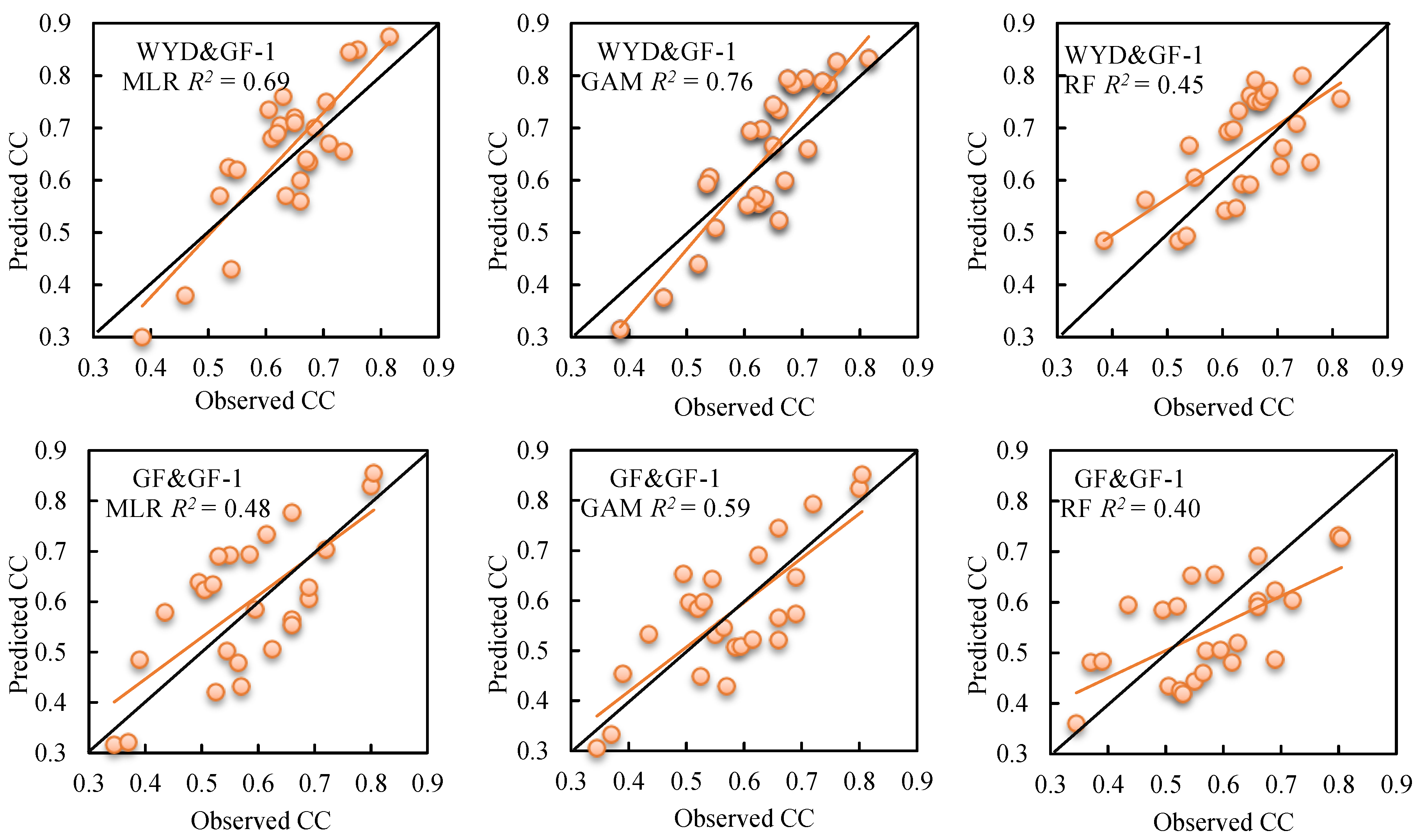
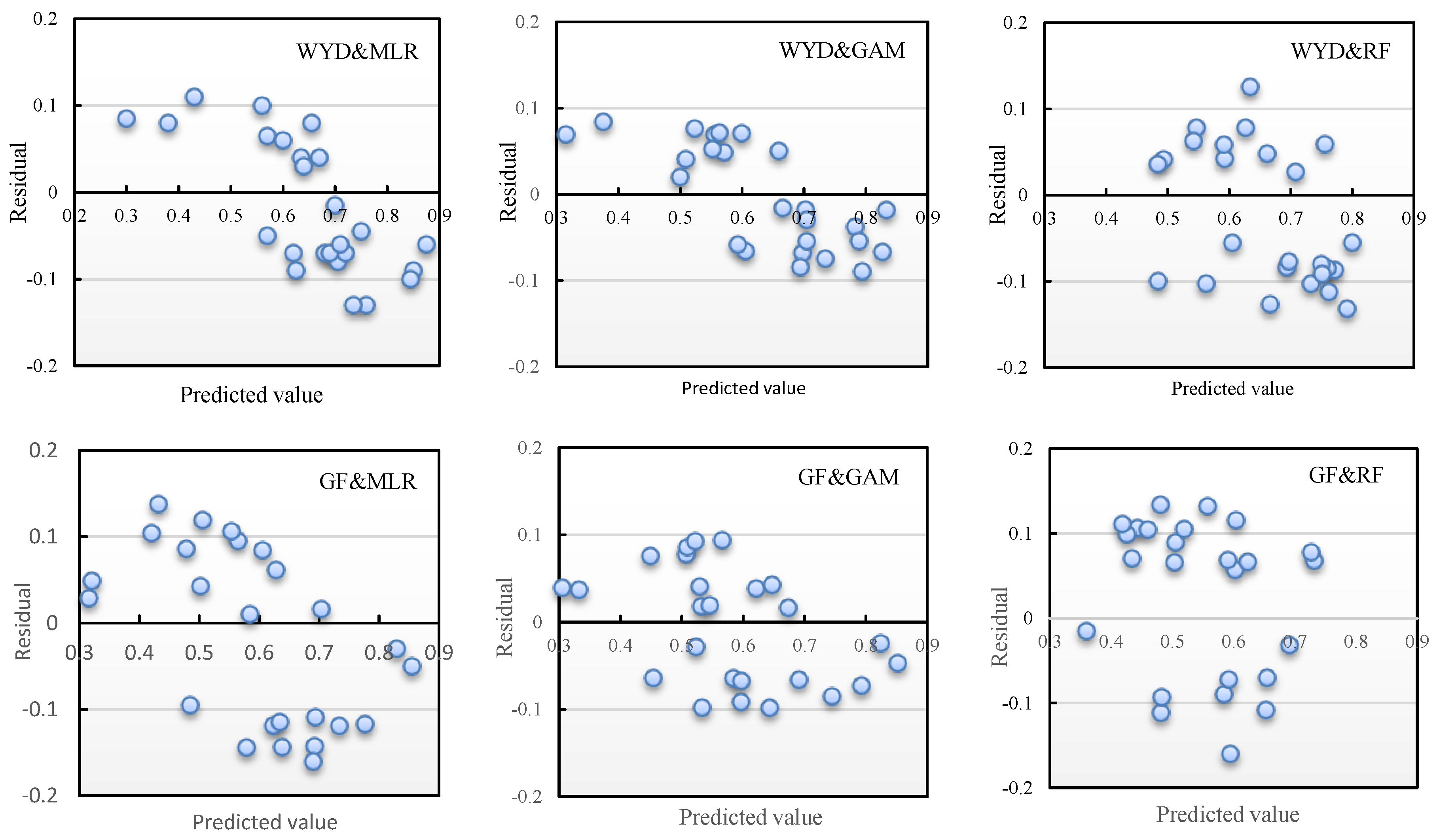
| Test Area | Model | Model Form | R2 | RMSE | rRMSE |
|---|---|---|---|---|---|
| WYD (Wangyedian) | MLR | CC = −96.55× DVI + 6.79× NIR + 240.73× RDVI − 0.37× RVI−106.85× SAVI + 47.37× SR − 37.85 | 0.69 | 0.0843 | 13.31% |
| GAM | CC = f(RDVI) + f(RVI) + f(NIR) + 0.60 | 0.76 | 0.0632 | 9.98% | |
| RF | CC = f(GREEN, NIR, DVI, RVI, SR, NDVI, RDVI, PVI, SAVI, MSAVI) | 0.45 | 0.0953 | 15.05% | |
| GF (Gaofeng) | MLR | CC = −3666.73×DVI + 34.00×MSAVI − 1813.71×NDVI + 22.25×NIR + 10430.38×RDVI − 5020.57×SAVI − 1.03 | 0.48 | 0.1018 | 17.61% |
| GAM | CC = f(DVI) + f(PVI) + f(NIR) + 0.58 | 0.59 | 0.0967 | 16.73% | |
| RF | CC = f(GREEN, NIR, DVI, RVI, SR, NDVI, RDVI, PVI, SAVI, MSAVI) | 0.40 | 0.1152 | 19.93% |
| Data Source | R2 | RMSE | rRMSE% | Method | n | Reference |
|---|---|---|---|---|---|---|
| Aerial Multispectral Sensor | 0.79 | Parametric model (MLR) | 6 | Le´vesque (2003) [55] | ||
| SPOT5 | 0.68 | 0.06 | Parametric model (partial least squares) | 39 | Wolter et al. (2009) [31] | |
| SPOT5 | 0.52 | 0.05 | Parametric model (partial least squares) | 40 | Wolter et al. (2009) [31] | |
| Sentinel-2A MSI | 0.69 | 0.11 | 16.0 | Semiparametric model (GAM) | 19 | Korhonen et al. (2017) [13] |
| Landsat 8 OLI | 0.70 | 0.10 | 15.0 | Semiparametric model (GAM) | 19 | Korhonen et al. (2017) [13] |
| Landsat 8 OLI | 0.12 | 12.0 | Nonparametric model (RF) | 60 | Halperin et al. (2016) [9] | |
| RapidEye | 0.12 | 12.3 | Nonparametric model (RF) | 60 | Halperin et al. (2016) [9] | |
| Landsat+LiDAR | 0.66 | 0.07 | Nonparametric model (RF) | >100 | Ahmed et al. (2015) [33] | |
| Landsat 8 OLI | 0.13 | 14.2 | Nonparametric model (KNN) | 60 | Halperin et al. (2016) [9] | |
| RapidEye | 0.11 | 14.6 | Nonparametric model (KNN) | 60 | Halperin et al. (2016) [9] |
© 2020 by the authors. Licensee MDPI, Basel, Switzerland. This article is an open access article distributed under the terms and conditions of the Creative Commons Attribution (CC BY) license (http://creativecommons.org/licenses/by/4.0/).
Share and Cite
Li, J.; Mao, X. Comparison of Canopy Closure Estimation of Plantations Using Parametric, Semi-Parametric, and Non-Parametric Models Based on GF-1 Remote Sensing Images. Forests 2020, 11, 597. https://doi.org/10.3390/f11050597
Li J, Mao X. Comparison of Canopy Closure Estimation of Plantations Using Parametric, Semi-Parametric, and Non-Parametric Models Based on GF-1 Remote Sensing Images. Forests. 2020; 11(5):597. https://doi.org/10.3390/f11050597
Chicago/Turabian StyleLi, Jiarui, and Xuegang Mao. 2020. "Comparison of Canopy Closure Estimation of Plantations Using Parametric, Semi-Parametric, and Non-Parametric Models Based on GF-1 Remote Sensing Images" Forests 11, no. 5: 597. https://doi.org/10.3390/f11050597