Regional Variability of the Romanian Main Tree Species Growth Using National Forest Inventory Increment Cores


Abstract
:
1. Introduction
2. Methods
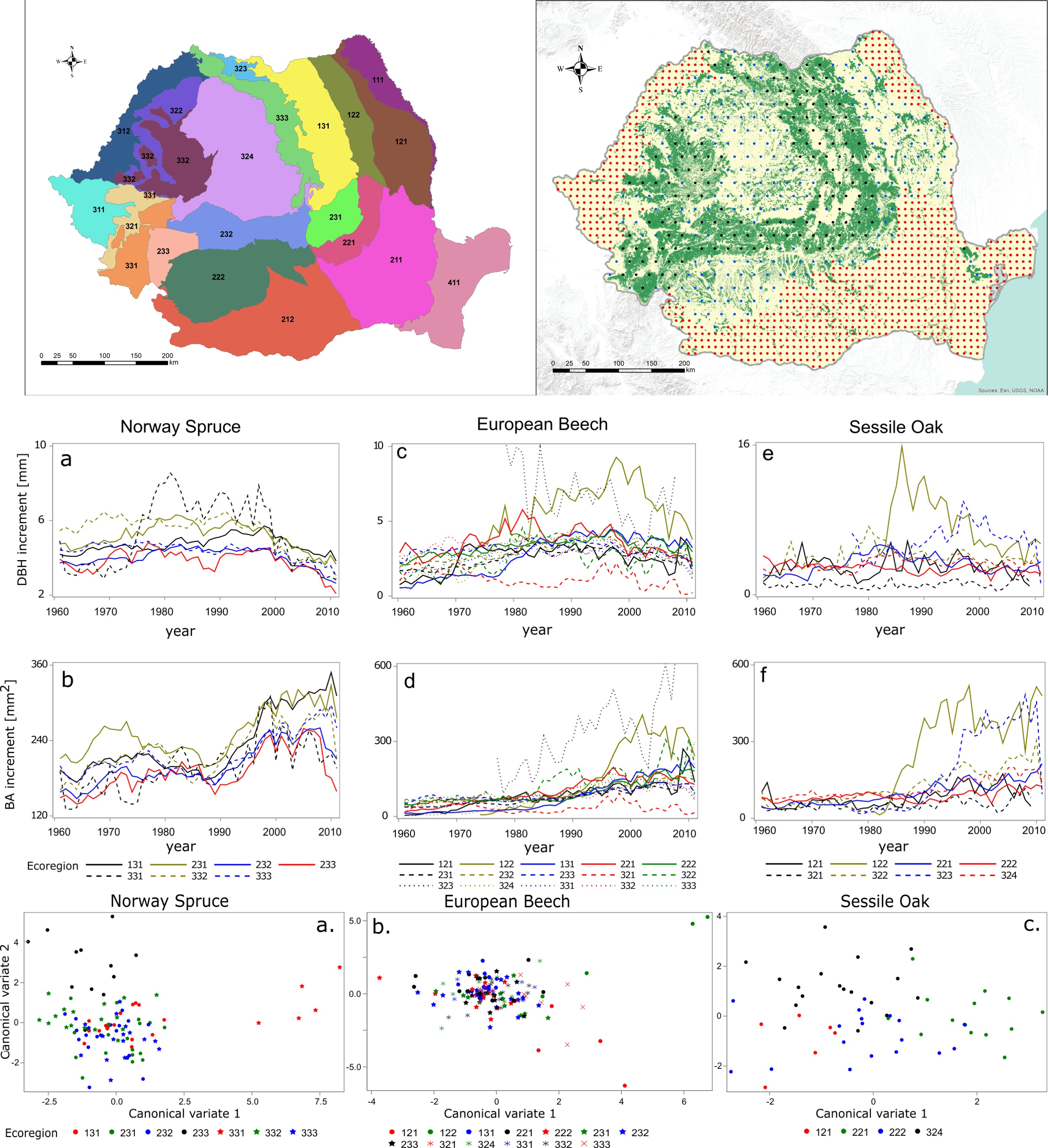
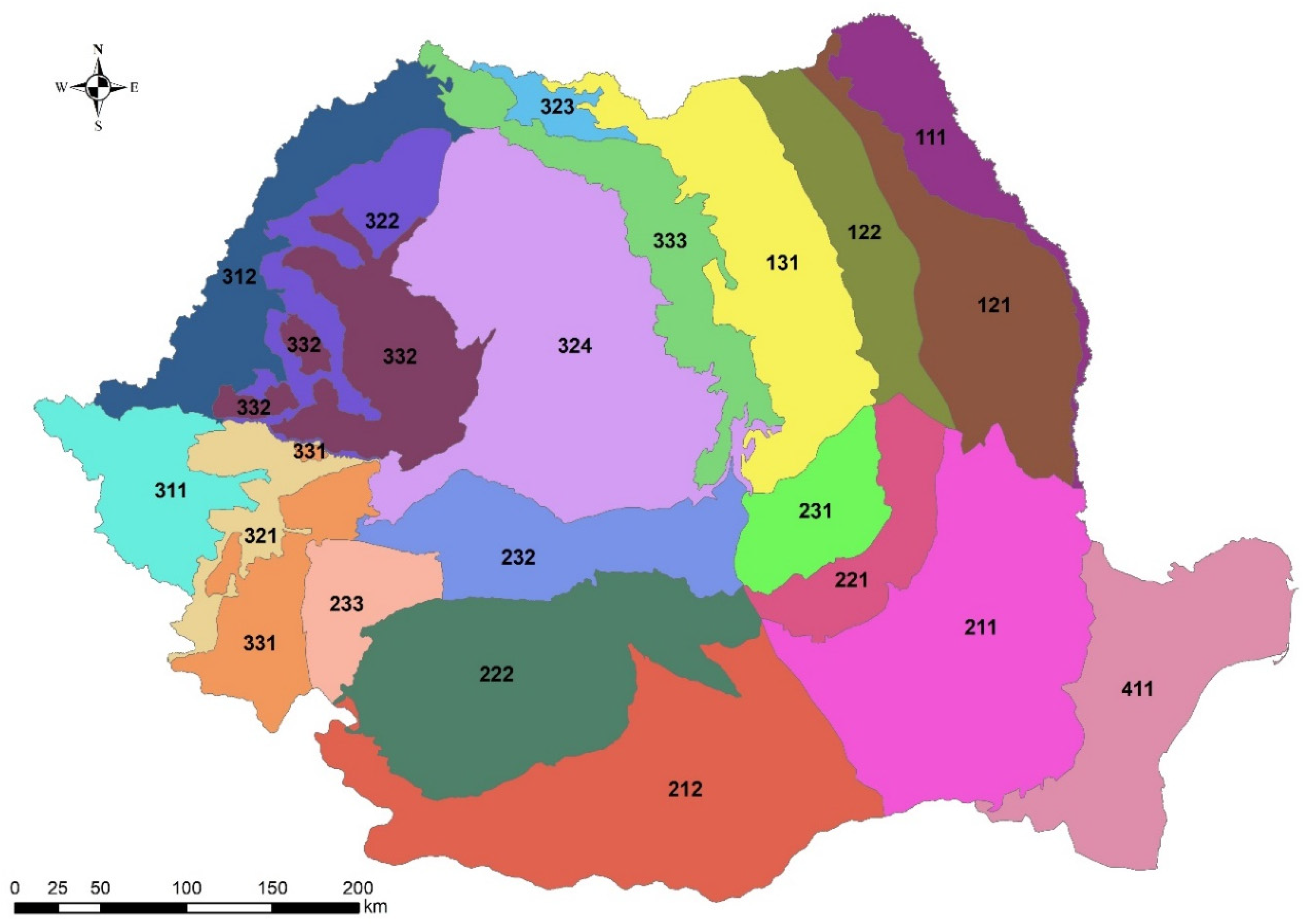
2.1. Romanian Ecoregions
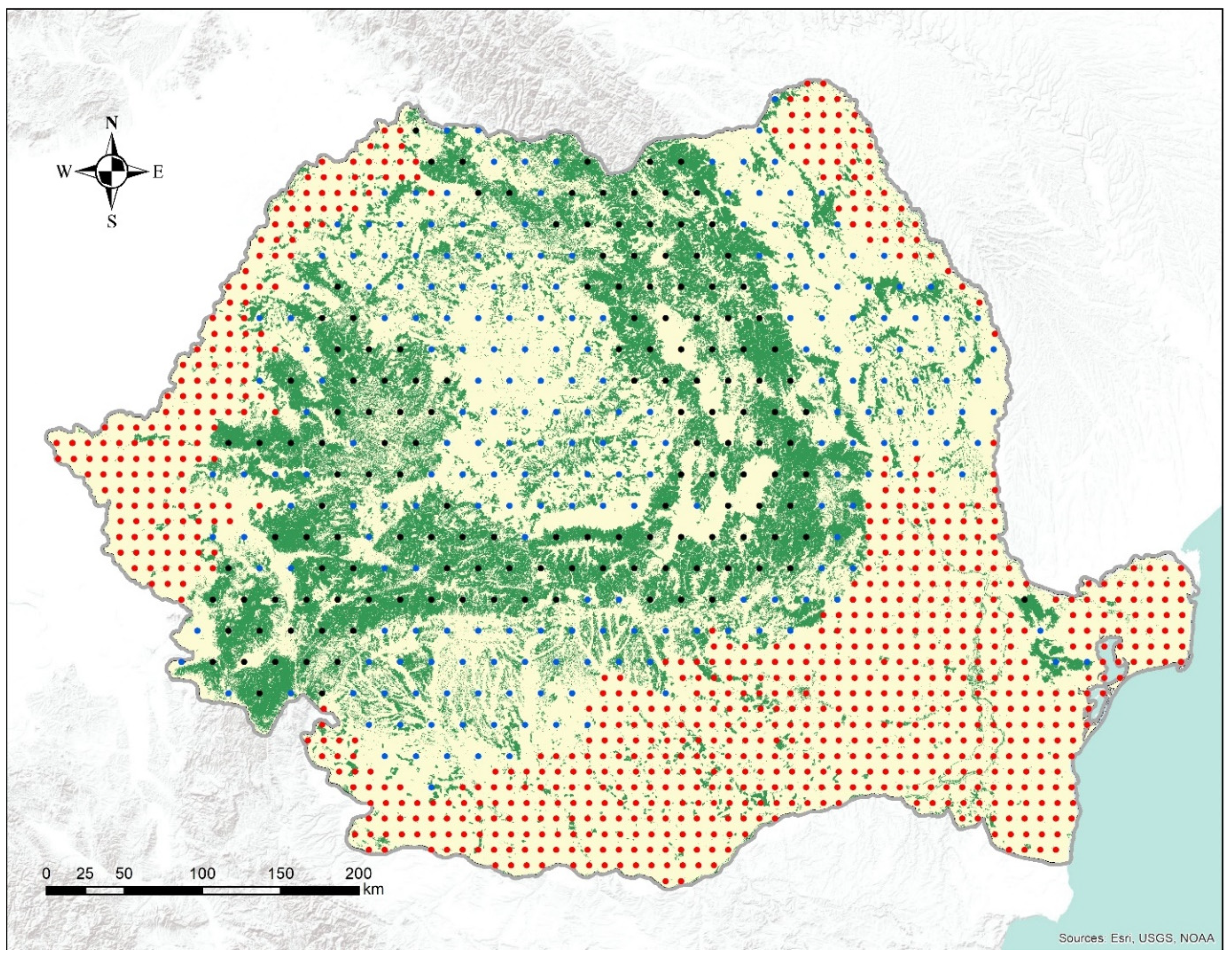
2.2. Increment Cores
2.3. Analysis
2.3.1. Mixed Models Analysis
2.3.2. Multivariate Analysis
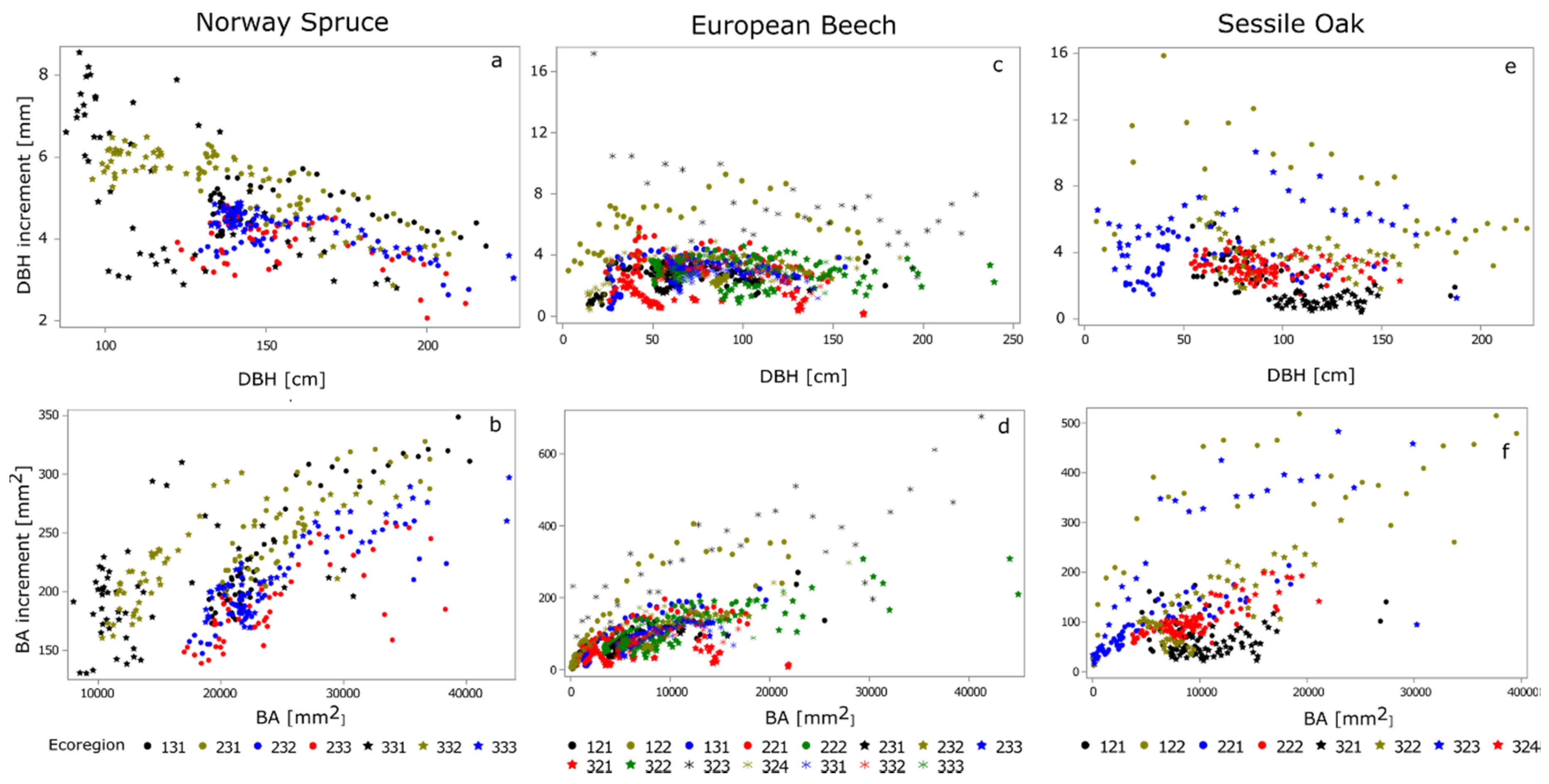
3. Results
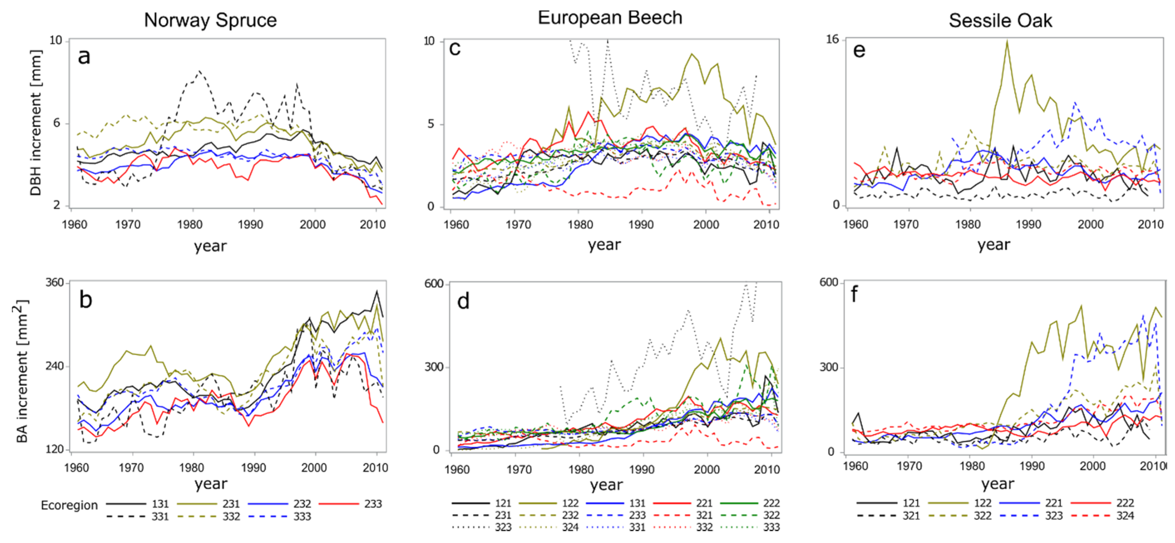
3.1. Mixed Models Analysis
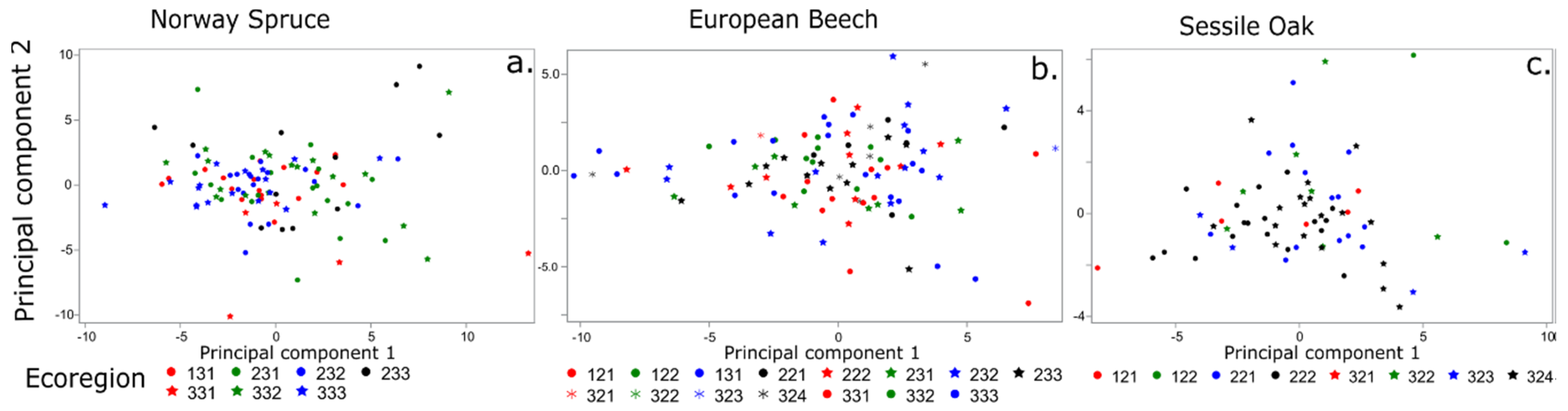
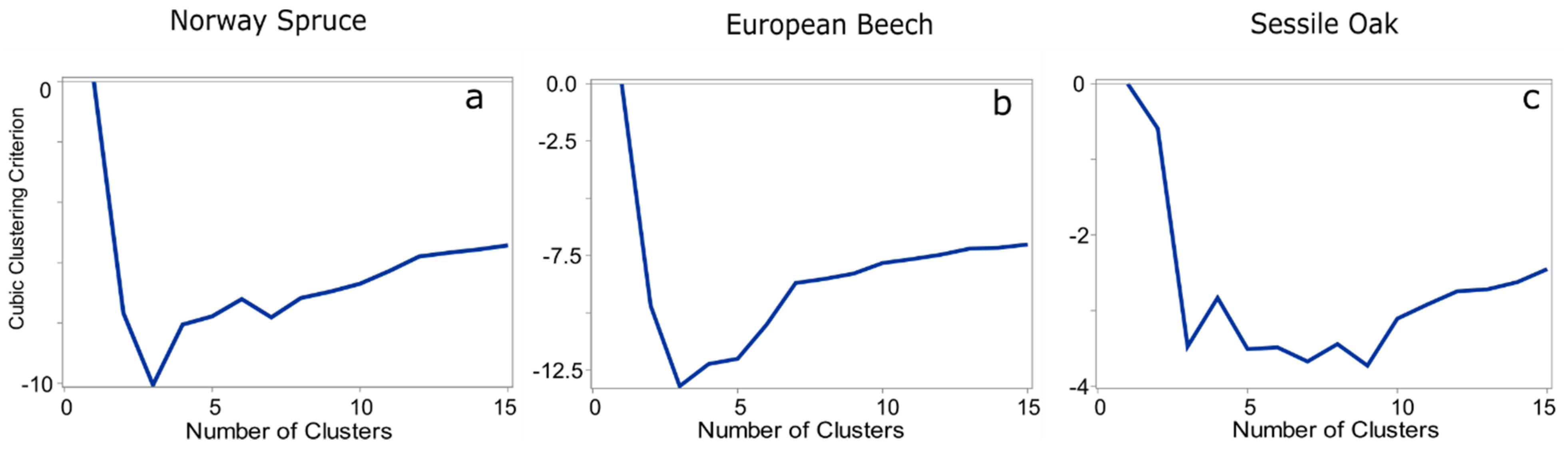
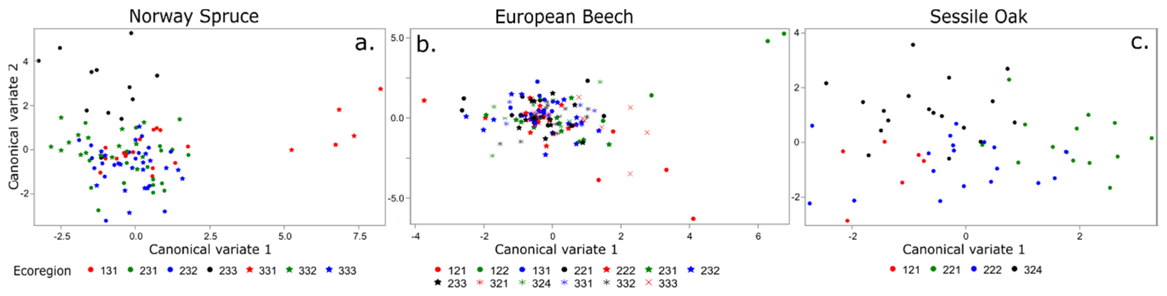
3.2. Multivariate Analysis
4. Discussion
5. Conclusions
Author Contributions
Acknowledgments
Conflicts of Interest
References
- Zianis, D.; Muukkonen, P.; Mäkipää, R.; Mencuccini, M. Biomass and Stem Volume Equations for Tree Species in Europe; Silva Fennica Monographs 4: Tampere, Finland, 2005. [Google Scholar]
- Bailey, R.G. Delineation of ecosystem regions. Environ. Manag. 1983, 7, 365–373. [Google Scholar] [CrossRef] [Green Version]
- Hughes, R.M.; Omernik, J.M. Ecological regions (ecoregions). In Environmental Geology; Springer: Dordrecht, The Netherlands, 1999; pp. 155–159. ISBN 978-1-4020-4494-6. [Google Scholar]
- Omernik, J.M. Perspectives on the nature and definition of ecological regions. Environ. Manag. 2004, 34, S27–S38. [Google Scholar] [CrossRef] [PubMed]
- Indreica, A.; Turtureanu, P.D.; Szabó, A.; Irimia, I. Romanian forest database: A phytosociological archive of woody vegetation. Phytocoenologia 2017, 47, 389–392. [Google Scholar] [CrossRef]
- Šijačić-Nikolić, M.; Milovanović, J.; Nonic, M. (Eds.) Forests of Southeast Europe under a Changing Climate: Conservation of Genetic Resources; Advances in Global Change Research; Springer International Publishing: Berlin/Heidelberg, Germany, 2019; ISBN 978-3-319-95266-6. [Google Scholar]
- Stapf, O. Conspectul Florei României. Nature 1899, 59, 221. [Google Scholar] [CrossRef] [Green Version]
- Bechtold, W.A.; Patterson, P.L. The Enhanced Forest Inventory and Analysis Program -National Sampling Design and Estimation Procedures; U.S. Department of Agriculture, Forest Service, Southern Research Station: Asheville, NC, USA, 2005; p. 85.
- Vidal, C.; Belouard, T.; Herve, J.C.; Rober, N.; Wolsak, J. A New Flexible Forest Inventory in France; USDA Forest Service: Portland, ME, USA, 2007; pp. 67–73.
- Tomppo, E.; Gschwantner, T.; Lawrence, M.; McRoberts, R.E. (Eds.) National Forest Inventories: Pathways for Common Reporting; Springer: Dordrecht, The Netherlands, 2010; ISBN 978-90-481-3232-4. [Google Scholar]
- IFN National Forest Inventory. Available online: https://roifn.ro/site/en/ (accessed on 6 August 2019).
- Marin, G.; Bouriaud, O.; Dumitru, M.; Nitu, D. Romania. In National Forest Inventories: Pathways for Common Reporting; Springer: Heidelberg, Germany, 2010; pp. 473–480. [Google Scholar]
- Charru, M.; Seynave, I.; Morneau, F.; Bontemps, J.-D. Recent changes in forest productivity: An analysis of national forest inventory data for common beech (Fagus sylvatica L.) in north-eastern France. For. Ecol. Manag. 2010, 260, 864–874. [Google Scholar] [CrossRef]
- Evans, M.E.K.; Falk, D.A.; Arizpe, A.; Swetnam, T.L.; Babst, F.; Holsinger, K.E. Fusing tree-ring and forest inventory data to infer influences on tree growth. Ecosphere 2017, 8, e01889. [Google Scholar] [CrossRef] [Green Version]
- Metsaranta, J.M. Dendrochronological procedures improve the precision and accuracy of tree and stand age estimates in the western Canadian boreal forest. For. Ecol. Manag. 2020, 457, 117657. [Google Scholar] [CrossRef]
- Marin, G.; Abrudan, I.; Strimbu, B.M. Increment cores of the National Forest Inventory from Romania. Math. Comput. For. Nat. Resour. Sci. 2019, 11, 294. [Google Scholar]
- Nyland, R.D. Silvicuture: Concepts and Applications; McGraw-Hill: New York, NY, USA, 1996. [Google Scholar]
- Kuglitsch, F.G.; Toreti, A.; Xoplaki, E.; Della-Marta, P.M.; Zerefos, C.S.; Türkeş, M.; Luterbacher, J. Heat wave changes in the eastern Mediterranean since 1960. Geophys. Res. Lett. 2010, 37. [Google Scholar] [CrossRef] [Green Version]
- Zuidhoff, F.S.; Kolstrup, E. Changes in palsa distribution in relation to climate change in Laivadalen, northern Sweden, especially 1960–1997. Permafr. Periglac. Process. 2000, 11, 55–69. [Google Scholar] [CrossRef]
- Gregory, P.J.; Marshall, B. Attribution of climate change: A methodology to estimate the potential contribution to increases in potato yield in Scotland since 1960. Glob. Chang. Biol. 2012, 18, 1372–1388. [Google Scholar] [CrossRef]
- Wang, S.; Zhang, M.; Li, Z.; Wang, F.; Li, H.; Li, Y.; Huang, X. Glacier area variation and climate change in the Chinese Tianshan Mountains since 1960. J. Geogr. Sci. 2011, 21, 263–273. [Google Scholar] [CrossRef]
- Yue, T.X.; Fan, Z.M.; Liu, J.Y. Changes of major terrestrial ecosystems in China since 1960. Glob. Planet. Chang. 2005, 48, 287–302. [Google Scholar] [CrossRef]
- Posmentier, E.S.; Cane, M.A.; Zebiak, S.E. Tropical pacific climate trends since 1960. J. Clim. 1989, 2, 731–736. [Google Scholar] [CrossRef] [Green Version]
- Husch, B.; Beers, T.W.; Kershaw, J.A. Forest Mensuration, 4th ed.; John Wiley and Sons: Hoboken, NJ, USA, 2002. [Google Scholar]
- Pretzsch, H. Forest Dynamics, Growth and Yield; Springer: Berlin, Germany, 2009. [Google Scholar]
- Weiskittel, A.R.; Hann, D.W.; Kershaw, J.A.; Vanclay, J.K. Forest Growth and Yield Modeling; Wiley-Blackwell: Chichester, UK, 2011; Volume 430. [Google Scholar]
- Crowder, M.J.; Hand, D.J. Analysis of Repeated Measures; Monographs on Statistics and Applied Probability; Chapman and Hall: London, UK, 1990. [Google Scholar]
- Fitzmaurice, G.M.; Laird, N.M.; Ware, J.H. Applied Longitudinal Analysis; Wiley: Hoboken, NJ, USA, 2004; ISBN 978-0-471-21487-8. [Google Scholar]
- Pinheiro, J.; Bates, D. Mixed Effects Models in S and S-PLUS; Springer: New York, NY, USA, 2000. [Google Scholar]
- Gotway, C.A.; Stroup, W.W. A generalized linear model approach to spatial data analysis and prediction. J. Agric. Biol. Environ. Stat. 1997, 2, 157–178. [Google Scholar] [CrossRef]
- Neter, J.; Kutner, M.H.; Nachtsheim, C.J.; Wasserman, W. Applied Linear Statistical Models; WCB McGraw-Hill: Boston, MA, USA, 1996. [Google Scholar]
- SAS Institute. SAS® 9.4; SAS Institute Inc.: Cary, NC, USA, 2013. [Google Scholar]
- Rencher, A.C. Methods of Multivariate Analysis; John Wiley and Sons: New York, NY, USA, 2002. [Google Scholar]
- Hardle, W.; Simar, L. Applied Multivariate Statistical Analysis; Springer: New York, NY, USA, 2003. [Google Scholar]
- Tabachnick, B.G.; Fidell, L.S. Using Multivariate Statistics; Allyn and Bacon: Needham Heights, MA, USA, 2001. [Google Scholar]
- Strimbu, B.M.; Hickey, G.M.; Strimbu, V.G.; Innes, J.L. On the use of statistical tests with non-normally distributed data in landscape change detection. For. Sci. 2009, 55, 72–83. [Google Scholar]
- Seppelt, R.; Richter, O. “It was an artefact not the result”: A note on systems dynamic model development tools. Environ. Model. Softw. 2005, 20, 1543–1548. [Google Scholar] [CrossRef]
- Oliver, C.D.; Larson, B.C. Forest Stand Dynamics, updated ed.; John Wiley & Sons, Inc.: New York, NY, USA, 1996; ISBN 978-0-471-13833-4. [Google Scholar]
- Hasenauer, H. Concepts within tree growth modeling. In Sustainable Forest Management: Growth Models for Europe; Hasenauer, H., Ed.; Springer Berlin Heidelberg: Berlin/Heidelberg, Germany, 2006; pp. 3–17. ISBN 978-3-540-31304-5. [Google Scholar]
- Strimbu, V.C.; Bokalo, M.; Comeau, P.G. Deterministic models of growth and mortality for jack pine in boreal forests of western Canada. Forests 2017, 8, 410. [Google Scholar] [CrossRef] [Green Version]
- Taylor, A.R.; Chen, H.Y.H.; VanDamme, L. A review of forest succession models and their suitability for forest management planning. For. Sci. 2009, 55, 23–36. [Google Scholar]
- Savva, Y.; Oleksyn, J.; Reich, P.B.; Tjoelker, M.G.; Vaganov, E.A.; Modrzynski, J. Interannual growth response of Norway spruce to climate along an altitudinal gradient in the Tatra Mountains, Poland. Trees 2006, 20, 735–746. [Google Scholar] [CrossRef]
- Andreassen, K.; Solberg, S.; Tveito, O.E.; Lystad, S.L. Regional differences in climatic responses of Norway spruce (Picea abies L. Karst) growth in Norway. For. Ecol. Manag. 2006, 222, 211–221. [Google Scholar] [CrossRef]
- Kramer, K.; Leinonen, I.; Loustau, D. The importance of phenology for the evaluation of impact of climate change on growth of boreal, temperate and Mediterranean forests ecosystems: An overview. Int. J. Biometeorol. 2000, 44, 67–75. [Google Scholar] [CrossRef] [PubMed]
- Zhang, Q.; Alfaro, R.I.; Hebda, R.J. Dendroecological studies of tree growth, climate and spruce beetle outbreaks in Central British Columbia, Canada. For. Ecol. Manag. 1999, 121, 215–225. [Google Scholar] [CrossRef]
- Shifley, S.R. A Generalized System of Models Forecasting Central States Tree Growth; Research Paper NC-279; US Department of Agriculture, Forest Service, North Central Forest Experiment Station: St. Paul, MN, USA, 1987; Volume 279.
- West, P.W. Use of diameter increment and basal area increment in tree growth studies. Can. J. For. Res. 1980, 10, 71–77. [Google Scholar] [CrossRef]
- Russell, M.B.; Weiskittel, A.R.; Kershaw, J.A., Jr. Comparing strategies for modeling individual-tree height and height-to-crown base increment in mixed-species Acadian forests of northeastern North America. Eur. J. For. Res. 2014, 133, 1121–1135. [Google Scholar] [CrossRef]
- Griffiths, R.P.; Madritch, M.D.; Swanson, A.K. The effects of topography on forest soil characteristics in the Oregon Cascade Mountains (USA): Implications for the effects of climate change on soil properties. For. Ecol. Manag. 2009, 257, 1–7. [Google Scholar] [CrossRef]
- Sandel, B.; Svenning, J.-C. Human impacts drive a global topographic signature in tree cover. Nat. Commun. 2013, 4, 2474. [Google Scholar] [CrossRef] [Green Version]
- Laubhann, D.; Sterba, H.; Reinds, G.J.; De Vries, W. The impact of atmospheric deposition and climate on forest growth in European monitoring plots: An individual tree growth model. For. Ecol. Manag. 2009, 258, 1751–1761. [Google Scholar] [CrossRef]
- Scharnweber, T.; Manthey, M.; Criegee, C.; Bauwe, A.; Schröder, C.; Wilmking, M. Drought matters–Declining precipitation influences growth of Fagus sylvatica L. and Quercus robur L. in north-eastern Germany. For. Ecol. Manag. 2011, 262, 947–961. [Google Scholar] [CrossRef]
- Toledo, M.; Poorter, L.; Peña-Claros, M.; Alarcón, A.; Balcázar, J.; Leaño, C.; Licona, J.C.; Llanque, O.; Vroomans, V.; Zuidema, P.; et al. Climate is a stronger driver of tree and forest growth rates than soil and disturbance. J. Ecol. 2011, 99, 254–264. [Google Scholar] [CrossRef]
- Adams, H.R.; Barnard, H.R.; Loomis, A.K. Topography alters tree growth–climate relationships in a semi-arid forested catchment. Ecosphere 2014, 5, art148. [Google Scholar] [CrossRef]
- Tardif, J.; Camarero, J.J.; Ribas, M.; Gutiérrez, E. Spatiotemporal variability in tree growth in the central pyrenees: climatic and site influences. Ecol. Monogr. 2003, 73, 241–257. [Google Scholar] [CrossRef] [Green Version]
- Spiecker, H. Tree rings and forest management in Europe. Dendrochronologia 2002, 20, 191–202. [Google Scholar] [CrossRef]


| Ecoregion Name | Ecoregion Code | Soil | Geomorphology | Geology | Province | Area [ha] |
|---|---|---|---|---|---|---|
| Moldavian Plateau | 121 | Chernozems, Phaezems, Luvisols, Fluvisols, Gleysols | Plateau | Sands, Gravels, Marls, Loess, Sandstones | Moldavia | 1,352,075 |
| Moldavian Hills | 122 | Luvisols, Eutric Cambisols, Phaezems | Hills | Marls, Calcarous Marls, Sandstones, Conglomerates, Tuffs | Moldavia | 806,488 |
| Eastern Carpathians | 131 | Eutric Cambisols, Dystric Cambisols, Entic podzols, Haplic podzol, Rendzic leptosol | Mountains | Flysch deposits | Moldavia | 1,546,525 |
| Buzau-Vrancea piedmonts | 221 | Regosols, Luvisols, Eutric Cambisols | Hills | Sands, Clay-sands, Marls, Sandstones, Limestones | Moldavia | 595,917 |
| Getic plateau | 222 | Chernozems, Phaezems, Luvisols, Eutric Cambisols, Vertisols, Fluvisols, Gleysols | Plateau | Marls, Sandy-marls, Sandstones, Tuffs, Sands, Gravels, Loess, | Muntenia | 1,934,478 |
| Buzau-Vrancea mountains | 231 | Dystric Cambisols Eutric Cambisols | Mountains | Flysch deposits Conglomerates | Muntenia | 550,591 |
| East Southern Carpathians | 232 | Dystric Cambisols Entic podzols, Haplic podzol, Rendzic leptosol | Mountains | Schists, Phyllites, Gneiss, Conglomerates, Limestones, | Muntenia | 1,028,094 |
| West Southern Carpathians | 233 | Dystric Cambisols Eutric Cambisols, Entic podzols, Haplic podzol, Rendzic leptosol | Mountains | Limestones, Schists, Phyllites, Granites | Muntenia | 449,804 |
| Caras Hills | 321 | Luvisols, Vertisols | Hills | Argillaceous marls, Sands, Gravels | Banat | 444,045 |
| Cris Hills | 322 | Luvisols, Eutric Cambisols | Hills | Sands, Gravels, Loess deposits | Transylvania | 679,685 |
| Maramures plateau | 323 | Eutric Cambisols, Luvisols | Plateau | Marls, Tuffs, Sandstones | Transylvania | 161,904 |
| Transylvania Plateau | 324 | Luvisols, Phaezems, Chernozems | Plateau | Marls, Calcarous marls tuffs, Sandstones, Conglomerates | Transylvania | 2,798,764 |
| Banat Mountains | 331 | Eutric Cambisols, Luvisols, Dystric Cambisols, Entic podzols, Rendzic leptosol | Mountains | Schists, Granites, Gabbro, Limestones | Banat | 708,961 |
| Western Carpathians | 332 | Eutric Cambisols, Luvisols, Dystric Cambisols, Rendzic leptosol | Mountains | Schists, Gneiss, Granites, Limestones, Sandstones | Transylvania | 1,054,126 |
| Volcanic ridge | 333 | Andosols, Entic podzols | Mountains | Lahar deposits, Andesites | Transylvania | 950,029 |
| Number of Rings | Number of Increment Cores | |||||
|---|---|---|---|---|---|---|
| Ecoregion (code) | Norway Spruce | European Beech | Sessile Oak | Norway Spruce | European Beech | Sessile Oak |
| Moldavian Plateau (121) | 2881 | 6575 | 41 | 93 | ||
| Moldavian Hills (122) | 8687 | 2385 | 112 | 29 | ||
| Eastern Carpathians (131) | 49,576 | 2286 | 986 | 332 | ||
| Buzau-Vrancea piedmonts (221) | 11,572 | 4400 | 142 | 87 | ||
| Getic plateau (222) | 15,496 | 13,962 | 223 | 219 | ||
| Buzau-Vrancea mountains (231) | 15,749 | 24,447 | 336 | 292 | ||
| East Southern Carpathians (232) | 27,969 | 30,700 | 506 | 387 | ||
| West Southern Carpathians (233) | 4259 | 20,280 | 84 | 258 | ||
| Caras Hills (321) | 1577 | 1419 | 20 | 17 | ||
| Cris Hills (322) | 2379 | 2969 | 31 | 44 | ||
| Maramures plateau (323) | 272 | 706 | 4 | 11 | ||
| Transylvania Plateau (324) | 13,763 | 17,075 | 187 | 253 | ||
| Banat Mountains (331) | 1654 | 36,007 | 47 | 427 | ||
| Western Carpathians (332) | 9102 | 21,448 | 228 | 285 | ||
| Volcanic ridge (333) | 28,595 | 23,445 | 568 | 287 | ||
| Total | 136,904 | 241,240 | 49,491 | 2755 | 3028 | 753 |
| Ecoregion Name | Norway Spruce | European Beech | Sessile Oak | |||
|---|---|---|---|---|---|---|
| DBHi [mm] | BAi [mm2] | DBHi [mm] | BAi [mm2] | DBHi [mm] | BAi [mm2] | |
| Moldavian Plateau (121) | 2.62 (1.655) | 86.20 (136.97) | 3.06 (1.282) | 87.46 (82.572) | ||
| Moldavian Hills (122) | 6.65 (1.419) | 223.12 (168.848) | 7.7 (1.696) | 343.7 (158.178) | ||
| Eastern Carpathians (131) | 4.81 (1.790) | 242.41 (183.54) | 3.26 (1.437) | 95.93 (119.595) | ||
| Buzau-Vrancea piedmonts (221) | 3.79 (1.291) | 116.32 (99.491) | 3.45 (1.514) | 109.59 (110.656) | ||
| Getic plateau (222) | 3.49 (1.434) | 104.26 (111.399) | 2.78 (1.160) | 86.88 (79.274) | ||
| Buzau-Vrancea mountains (231) | 5.21 (1.796) | 259.18 (174.2) | 2.68 (1.266) | 79.63 (93.75) | ||
| East Southern Carpathians (232) | 4.06 (1.552) | 205.57 (148.561) | 3.19 (1.293) | 103.07 (99.455) | ||
| West Southern Carpathians (233) | 3.87 (1.663) | 195.75 (162.814) | 3.21 (1.214) | 93.28 (89.638) | ||
| Caras Hills (321) | 1.23 (0.939) | 35.37 (66.591) | 1.08 (0.197) | 51.65 (22.047) | ||
| Cris Hills (322) | 2.63 (1.414) | 123.64 (129.655) | 4.15 (1.498) | 144.01 (116.801) | ||
| Maramures plateau (323) | 7.16 (1.336) | 327.48 (143.497) | 6.13 (1.738) | 230.53 (232.496) | ||
| Transylvania Plateau (324) | 3.32 (1.418) | 98.47 (118.498) | 3.4 (1.392) | 120.2 (114.688) | ||
| Banat Mountains (331) | 5.52 (1.848) | 218.39 (172.912) | 2.64 (1.331) | 82.91 (97.022) | ||
| Western Carpathians (332) | 5.27 (1.699) | 236.36 (167.421) | 3.09 (1.158) | 88.88 (82.883) | ||
| Volcanic ridge (333) | 4.35 (1.570) | 220.25 (161.321) | 3.27 (1.502) | 108.19 (125.989) | ||
| Ecoregion | 131 | 231 | 232 | 233 | 331 | 332 | 333 |
|---|---|---|---|---|---|---|---|
| 131 | |||||||
| 231 | DBHi | ||||||
| 232 | BAi | ||||||
| 233 | DBHi/BAi | DBHi | DBHi | ||||
| 331 | DBHi | DBHi | |||||
| 332 | DBHi | ||||||
| 333 |
| Ecoregion | 121 | 122 | 131 | 221 | 222 | 231 | 232 | 233 | 321 | 322 | 323 | 324 | 331 | 332 | 333 |
|---|---|---|---|---|---|---|---|---|---|---|---|---|---|---|---|
| 121 | DBHi/BAi | DBHi | |||||||||||||
| 122 | DBHi | DBHi | |||||||||||||
| 131 | DBHi/BAi | DBHi | DBHi/BAi | ||||||||||||
| 221 | BAi | DBHi/BAi | DBHi | DBHi | |||||||||||
| 222 | DBHi/BAi | DBHi/BAi | BAi | DBHi/BAi | |||||||||||
| 231 | BAi | ||||||||||||||
| 232 | DBHi/BAi | BAi | DBHi | ||||||||||||
| 233 | DBHi/BAi | ||||||||||||||
| 321 | DBHi/BAi | DBHi | DBHi/BAi | ||||||||||||
| 322 | |||||||||||||||
| 323 | |||||||||||||||
| 324 | |||||||||||||||
| 331 | DBHi | ||||||||||||||
| 332 | |||||||||||||||
| 333 |
| Ecoregion | 121 | 122 | 221 | 222 | 321 | 322 | 323 | 324 |
|---|---|---|---|---|---|---|---|---|
| 121 | ||||||||
| 122 | ||||||||
| 221 | DBHi/BAi | DBHi | DBHi | |||||
| 222 | DBHi | |||||||
| 321 | DBHi/BAi | DBHi/BAi | ||||||
| 322 | DBHi | |||||||
| 323 | ||||||||
| 324 |
| Species | Groups of Ecoregions | Minimum Difference among Groups | % of Variation Explained | |
|---|---|---|---|---|
| DBHi | BAi | |||
| Norway spruce | 3 | 0.29 | 83.7 | 91.8 |
| European beech | 3 | 0.25 | 70.1 | 83.2 |
| Sessile oak | 3 | 0.25 | 71.5 | 87.5 |
© 2020 by the authors. Licensee MDPI, Basel, Switzerland. This article is an open access article distributed under the terms and conditions of the Creative Commons Attribution (CC BY) license (http://creativecommons.org/licenses/by/4.0/).
Share and Cite
Marin, G.; Strimbu, V.C.; Abrudan, I.V.; Strimbu, B.M. Regional Variability of the Romanian Main Tree Species Growth Using National Forest Inventory Increment Cores. Forests 2020, 11, 409. https://doi.org/10.3390/f11040409
Marin G, Strimbu VC, Abrudan IV, Strimbu BM. Regional Variability of the Romanian Main Tree Species Growth Using National Forest Inventory Increment Cores. Forests. 2020; 11(4):409. https://doi.org/10.3390/f11040409
Chicago/Turabian StyleMarin, Gheorghe, Vlad C. Strimbu, Ioan V. Abrudan, and Bogdan M. Strimbu. 2020. "Regional Variability of the Romanian Main Tree Species Growth Using National Forest Inventory Increment Cores" Forests 11, no. 4: 409. https://doi.org/10.3390/f11040409