Comparison of GF2 and SPOT6 Imagery on Canopy Cover Estimating in Northern Subtropics Forest in China

 ,
,
Abstract
:1. Introduction
2. Materials and Methods
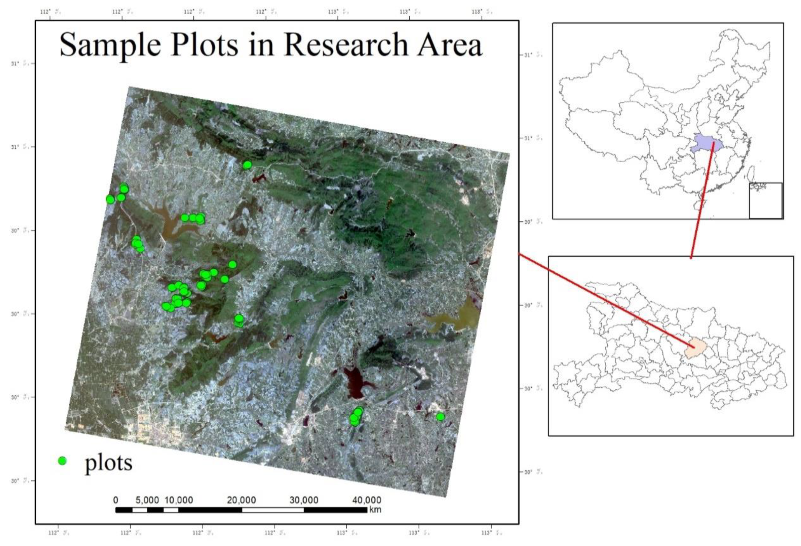
2.1. Study Area
2.2. Data
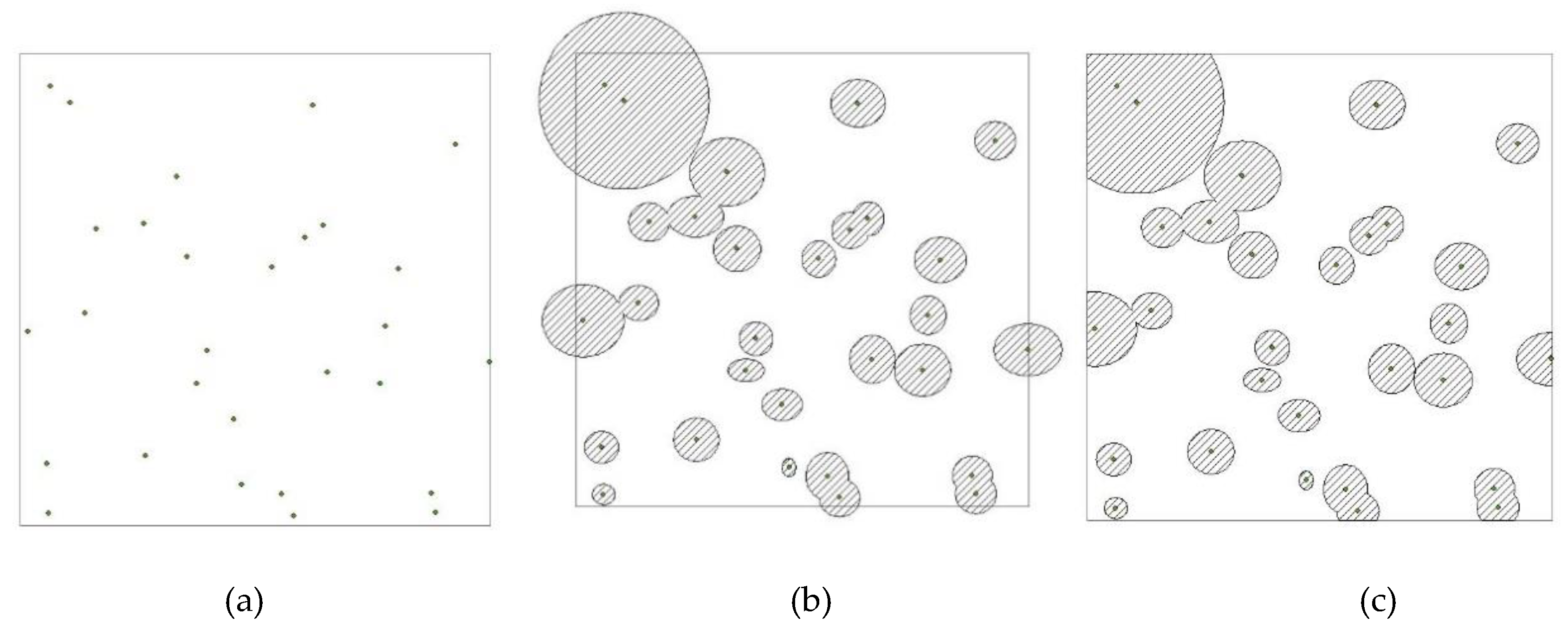
2.2.1. Field Data
2.2.2. Remote Sensing imagery
2.2.3. Predictor Variables
2.3. Modeling Methods
2.4. Model Evaluations
3. Results
3.1. Canopy Cover Characteristics in Different Forest Types
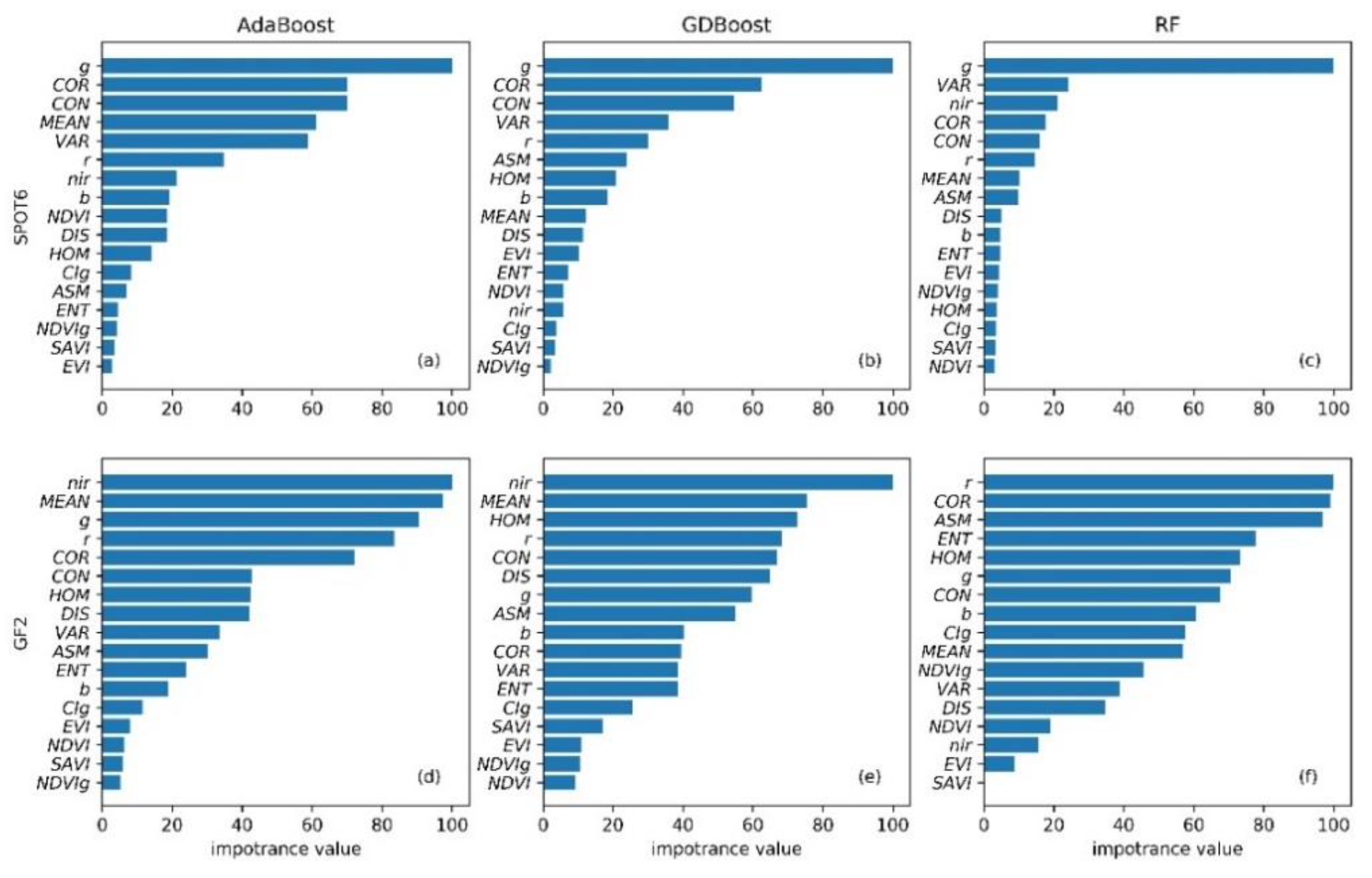
3.2. Assess the Relative Importance Value of Predictors for the Three Models
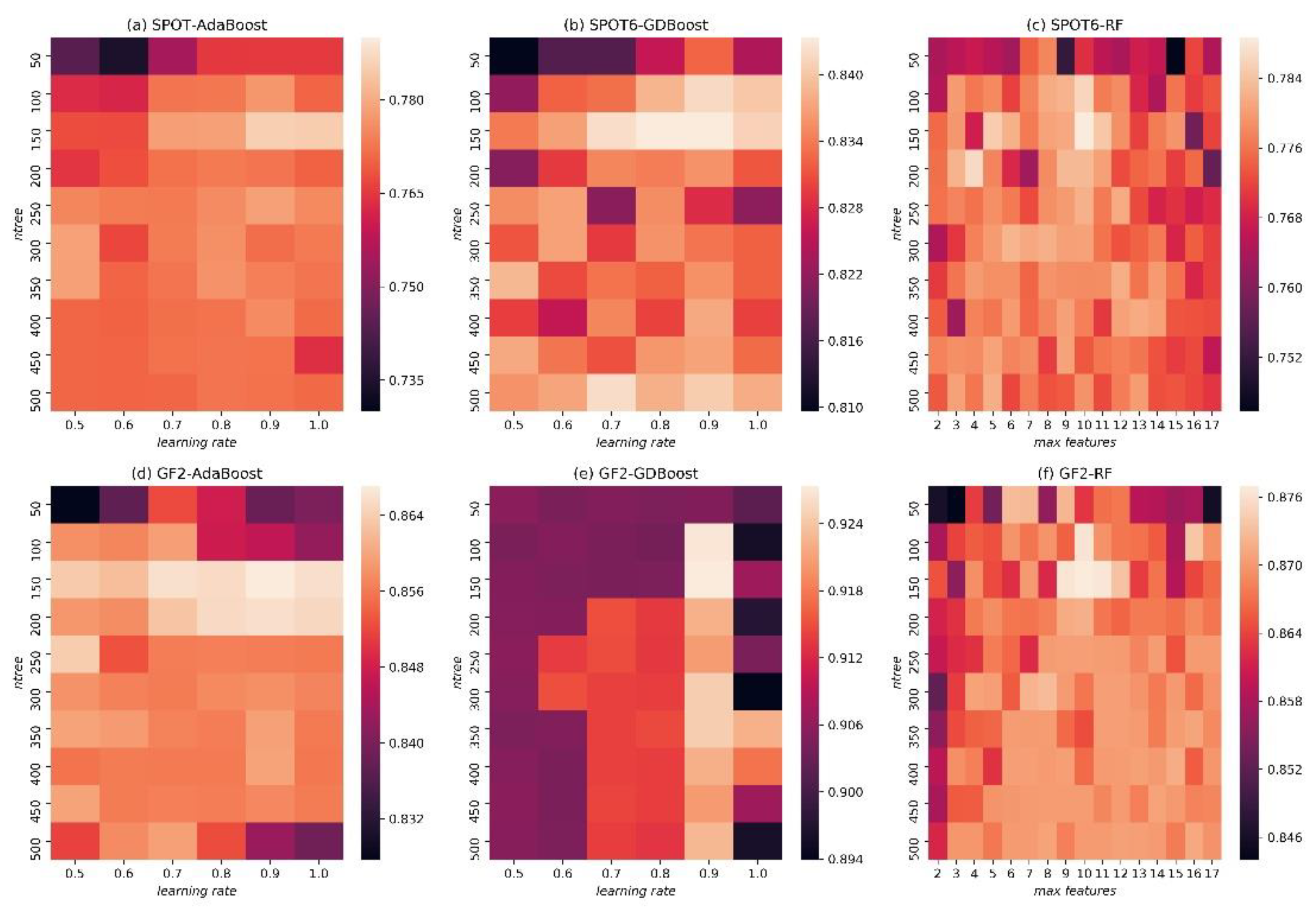
3.3. Parameter Tuning for Models
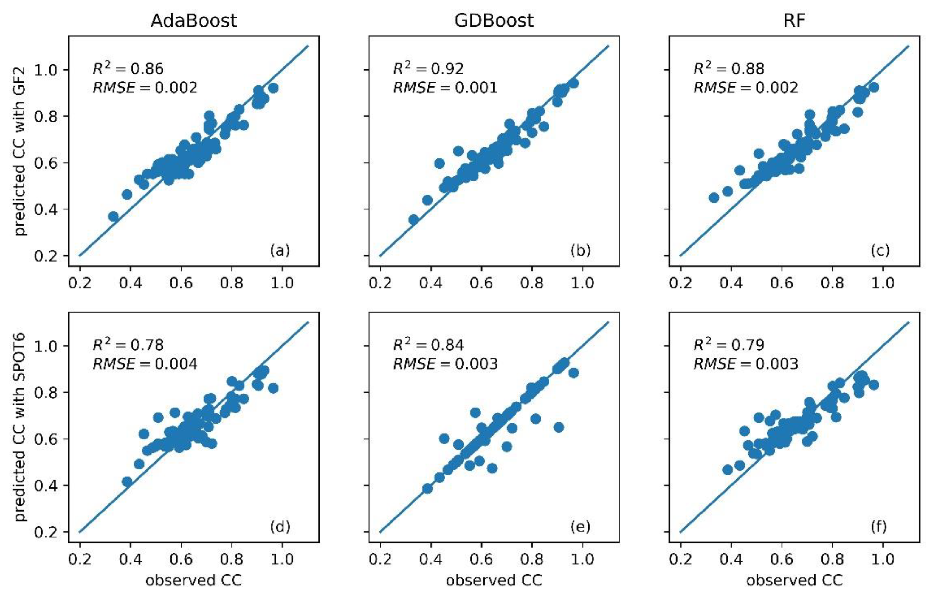
3.4. Canopy Cover Estimation Accuracy
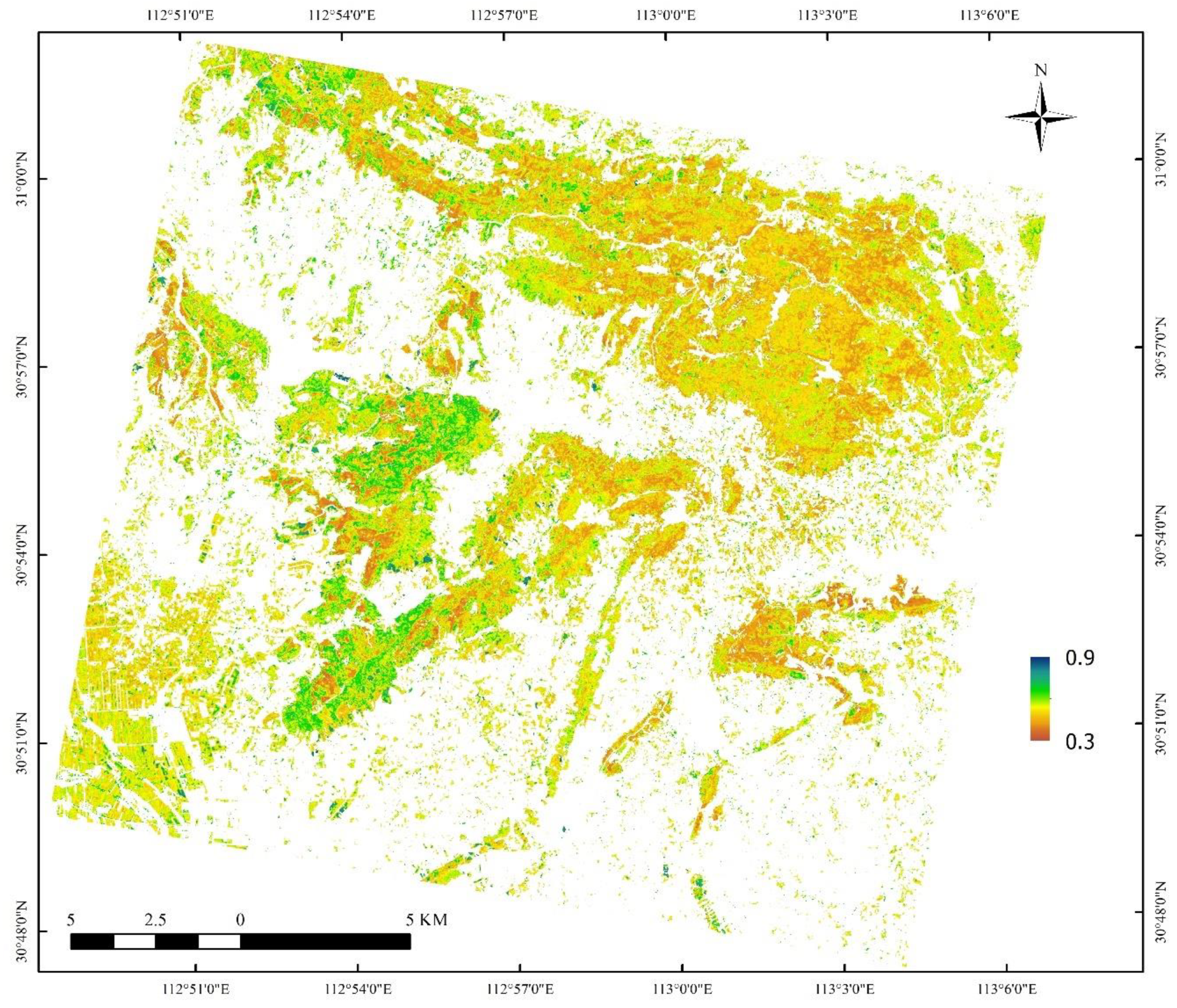
3.5. Mapping Results
4. Discussion
5. Conclusions
Author Contributions
Funding
Acknowledgments
Conflicts of Interest
References
- Jennings, S.B.; Brown, N.D.; Sheil, D. Assessing forest canopies and understorey illumination: Canopy closure, canopy cover and other measures. For. Int. J. For. Res. 1999, 72, 59–74. [Google Scholar] [CrossRef]
- Tichý, L. Field test of canopy cover estimation by hemispherical photographs taken with a smartphone. J. Veg. Sci. 2016, 27, 427–435. [Google Scholar] [CrossRef]
- Falkowski, M.J.; Evans, J.S.; Naugle, D.E.; Hagen, C.A.; Carleton, S.A.; Maestas, J.D.; Khalyani, A.H.; Poznanovic, A.J.; Lawrence, A.J. Mapping Tree Canopy Cover in Support of Proactive Prairie Grouse Conservation in Western North America. Rangel. Ecol. Manag. 2017, 70, 15–24. [Google Scholar] [CrossRef] [Green Version]
- Hansen, M.C.; DeFries, R.S.; Townshend, J.R.G.; Carroll, M.; Dimiceli, C.; Sohlberg, R.A. Global Percent Tree Cover at a Spatial Resolution of 500 Meters: First Results of the MODIS Vegetation Continuous Fields Algorithm. Earth Interact. 2003, 7, 1–15. [Google Scholar] [CrossRef] [Green Version]
- Huang, C.; Zhou, Z.; Wang, D.; Dian, Y. Monitoring forest dynamics with multi-scale and time series imagery. Environ. Monit. Assess. 2016, 188, 273. [Google Scholar] [CrossRef] [PubMed]
- Monsef, H.A.-E.; Smith, S.E. A new approach for estimating mangrove canopy cover using Landsat 8 imagery. Comput. Electron. Agric. 2017, 135, 183–194. [Google Scholar] [CrossRef]
- Halperin, J.; LeMay, V.; Coops, N.; Verchot, L.; Marshall, P.; Lochhead, K. Canopy cover estimation in miombo woodlands of Zambia: Comparison of Landsat 8 OLI versus RapidEye imagery using parametric, nonparametric, and semiparametric methods. Remote Sens. Environ. 2016, 179, 170–182. [Google Scholar] [CrossRef]
- Hilker, T.; Wulder, M.A.; Coops, N.C.; Seitz, N.; White, J.C.; Gao, F.; Masek, J.G.; Stenhouse, G. Generation of dense time series synthetic Landsat data through data blending with MODIS using a spatial and temporal adaptive reflectance fusion model. Remote Sens. Environ. 2009, 113, 1988–1999. [Google Scholar] [CrossRef]
- Korhonen, L.; Packalen, P.; Rautiainen, M. Comparison of Sentinel-2 and Landsat 8 in the estimation of boreal forest canopy cover and leaf area index. Remote Sens. Environ. 2017, 195, 259–274. [Google Scholar] [CrossRef]
- Morrison, J.; Higginbottom, T.P.; Symeonakis, E.; Jones, M.J.; Omengo, F.; Walker, S.L.; Cain, B. Detecting Vegetation Change in Response to Confining Elephants in Forests Using MODIS Time-Series and BFAST. Remote Sens. 2018, 10, 1075. [Google Scholar] [CrossRef] [Green Version]
- Ruefenacht, B. Comparison of Three Landsat TM Compositing Methods: A Case Study Using Modeled Tree Canopy Cover. Photogramm. Eng. Remote Sens. 2016, 82, 199–211. [Google Scholar] [CrossRef]
- Chemura, A.; Mutanga, O.; Odindi, J. Empirical Modeling of Leaf Chlorophyll Content in Coffee (Coffea Arabica) Plantations With Sentinel-2 MSI Data: Effects of Spectral Settings, Spatial Resolution, and Crop Canopy Cover. IEEE J. Sel. Top. Appl. Earth Obs. Remote Sens. 2017, 10, 5541–5550. [Google Scholar] [CrossRef]
- Mu, X.; Song, W.; Gao, Z.; McVicar, T.R.; Donohue, R.J.; Yan, G. Fractional vegetation cover estimation by using multi-angle vegetation index. Remote Sens. Environ. 2018, 216, 44–56. [Google Scholar] [CrossRef]
- Schultz, M.; Clevers, J.G.P.W.; Carter, S.; Verbesselt, J.; Avitabile, V.; Quang, H.V.; Herold, M. Performance of vegetation indices from Landsat time series in deforestation monitoring. Int. J. Appl. Earth Obs. Geoinf. 2016, 52, 318–327. [Google Scholar] [CrossRef]
- Yu, W.; Li, J.; Liu, Q.; Zeng, Y.; Zhao, J.; Xu, B.; Yin, G. Global Land Cover Heterogeneity Characteristics at Moderate Resolution for Mixed Pixel Modeling and Inversion. Remote Sens. 2018, 10, 856. [Google Scholar] [CrossRef] [Green Version]
- Hauser, L.T.; Vu, G.N.; Nguyen, B.A.; Dade, E.; Nguyen, H.M.; Nguyen, T.T.Q.; Le, T.Q.; Vu, L.H.; Tong, A.T.H.; Pham, H.V. Uncovering the spatio-temporal dynamics of land cover change and fragmentation of mangroves in the Ca Mau peninsula, Vietnam using multi-temporal SPOT satellite imagery (2004–2013). Appl. Geogr. 2017, 86, 197–207. [Google Scholar] [CrossRef]
- Cheng, Y.; Jin, S.; Wang, M.; Zhu, Y.; Dong, Z. Image Mosaicking Approach for a Double-Camera System in the GaoFen2 Optical Remote Sensing Satellite Based on the Big Virtual Camera. Sensors 2017, 17, 1441. [Google Scholar] [CrossRef] [Green Version]
- Li, S.M.; Li, Z.Y.; Chen, E.X.; Liu, Q.W. Object-Based Forest Cover Monitoring Using Gaofen-2 High Resolution Satellite Images. ISPRS—Int. Arch. Photogramm. Remote Sens. Spat. Inf. Sci. 2016, XLI-B8, 1437–1440. [Google Scholar] [CrossRef] [Green Version]
- Tong, X.-Y.; Lu, Q.; Xia, G.-S.; Zhang, L. Large-scale Land Cover Classification in GaoFen-2 Satellite Imagery. arXiv 2018, arXiv:180600901 Cs. [Google Scholar]
- Mahoney, C.; Hopkinson, C. Continental Estimates of Canopy Gap Fraction by Active Remote Sensing. Can. J. Remote Sens. 2017, 43, 345–359. [Google Scholar] [CrossRef]
- Hu, T.; Su, Y.; Xue, B.; Liu, J.; Zhao, X.; Fang, J.; Guo, Q. Mapping Global Forest Aboveground Biomass with Spaceborne LiDAR, Optical Imagery, and Forest Inventory Data. Remote Sens. 2016, 8, 565. [Google Scholar] [CrossRef] [Green Version]
- Xu, M.; Liu, R.; Chen, J.M.; Liu, Y.; Shang, R.; Ju, W.; Wu, C.; Huang, W. Retrieving leaf chlorophyll content using a matrix-based vegetation index combination approach. Remote Sens. Environ. 2019, 224, 60–73. [Google Scholar] [CrossRef]
- Gitelson, A.A.; Kaufman, Y.J.; Merzlyak, M.N. Use of a green channel in remote sensing of global vegetation from EOS-MODIS. Remote Sens. Environ. 1996, 58, 289–298. [Google Scholar] [CrossRef]
- Gitelson, A.A.; Kaufman, Y.J.; Stark, R.; Rundquist, D. Novel algorithms for remote estimation of vegetation fraction. Remote Sens. Environ. 2002, 80, 76–87. [Google Scholar] [CrossRef] [Green Version]
- Heryadi, Y.; Miranda, E. Land Cover Classification Based on Sentinel-2 Satellite Imagery Using Convolutional Neural Network Model: A Case Study in Semarang Area, Indonesia. In Intelligent Information and Database Systems: Recent Developments; Huk, M., Maleszka, M., Szczerbicki, E., Eds.; Springer International Publishing: Cham, Switzerland, 2020; Volume 830, pp. 191–206. ISBN 978-3-030-14131-8. [Google Scholar]
- Dian, Y.; Li, Z.; Pang, Y. Spectral and Texture Features Combined for Forest Tree species Classification with Airborne Hyperspectral Imagery. J. Indian Soc. Remote Sens. 2014, 43, 101–107. [Google Scholar] [CrossRef]
- Zhao, Q.; Wang, F.; Zhao, J.; Zhou, J.; Yu, S.; Zhao, Z. Estimating Forest Canopy Cover in Black Locust (Robinia pseudoacacia L.) Plantations on the Loess Plateau Using Random Forest. Forests 2018, 9, 623. [Google Scholar] [CrossRef] [Green Version]
- Carreiras, J.M.B.; Pereira, J.M.C.; Pereira, J.S. Estimation of tree canopy cover in evergreen oak woodlands using remote sensing. For. Ecol. Manag. 2006, 223, 45–53. [Google Scholar] [CrossRef]
- Humagain, K.; Portillo-Quintero, C.; Cox, R.D.; Cain, J.W. Estimating forest canopy cover dynamics in Valles Caldera National Preserve, New Mexico, using LiDAR and Landsat data. Appl. Geogr. 2018, 99, 120–132. [Google Scholar] [CrossRef]
- Jia, K.; Liang, S.; Gu, X.; Baret, F.; Wei, X.; Wang, X.; Yao, Y.; Yang, L.; Li, Y. Fractional vegetation cover estimation algorithm for Chinese GF-1 wide field view data. Remote Sens. Environ. 2016, 177, 184–191. [Google Scholar] [CrossRef]
- LARSSON, H. Linear regressions for canopy cover estimation in Acacia woodlands using Landsat-TM, -MSS and SPOT HRV XS data. Int. J. Remote Sens. 1993, 14, 2129–2136. [Google Scholar] [CrossRef]
- Parmehr, E.G.; Amati, M.; Taylor, E.J.; Livesley, S.J. Estimation of urban tree canopy cover using random point sampling and remote sensing methods. Urban For. Urban Green. 2016, 20, 160–171. [Google Scholar] [CrossRef]
- Papadopoulos, S.; Azar, E.; Woon, W.-L.; Kontokosta, C.E. Evaluation of tree-based ensemble learning algorithms for building energy performance estimation. J. Build. Perform. Simul. 2018, 11, 322–332. [Google Scholar] [CrossRef]
- Pedregosa, F.; Varoquaux, G.; Gramfort, A.; Michel, V.; Thirion, B.; Grisel, O.; Blondel, M.; Prettenhofer, P.; Weiss, R.; Dubourg, V.; et al. Scikit-learn: Machine Learning in Python. J. Mach. Learn. Res. 2011, 12, 2825–2830. [Google Scholar]
- Ma, Q.; Su, Y.; Guo, Q. Comparison of Canopy Cover Estimations from Airborne LiDAR, Aerial Imagery, and Satellite Imagery. IEEE J. Sel. Top. Appl. Earth Obs. Remote Sens. 2017, 10, 4225–4236. [Google Scholar] [CrossRef]
- Mohamed, A.E.A. Mapping Tree Canopy Cover in the Semi-Arid Sahel Using Satellite Remote Sensing and Google Earth Imagery. Master’s Thesis, Lund University, Lund, Sweden, 2017. [Google Scholar]
- Hunt, E.R.; Hively, W.D.; McCarty, G.W.; Daughtry, C.S.T.; Forrestal, P.J.; Kratochvil, R.J.; Carr, J.L.; Allen, N.F.; Fox-Rabinovitz, J.R.; Miller, C.D. NIR-Green-Blue High-Resolution Digital Images for Assessment of Winter Cover Crop Biomass. GISci. Remote Sens. 2011, 48, 86–98. [Google Scholar] [CrossRef]


| SPOT6 | GF2 | |||
|---|---|---|---|---|
| Band | Wavelength (nm) | Resolution (m) | Wavelength (nm) | Resolution (m) |
| Blue (B) | 455–525 | 6.8 | 450–520 | 4 |
| Green (G) | 530–590 | 6.8 | 520–590 | 4 |
| Red (R) | 625–695 | 6.8 | 630–690 | 4 |
| Near infrared (NIR) | 760–890 | 6.8 | 770–890 | 4 |
| Panchromatic | 455–745 | 1.5 | 450–900 | 1 |
| Vegetation Indices (VIs) | Formula |
|---|---|
| 1. Normalized difference vegetation index (NDVI) | |
| 2. Normalized difference index using the green band (NDVIg) | |
| 3. Chlorophyll index using the green band (CIg) | |
| 4. Enhanced Vegetation Index (EVI) | |
| 5. Soil Adjusted Vegetation Index (SAVI) |
| Gray Level Co-Occurrence Matrix based Texture Parameter Estimation | Formula |
|---|---|
| 1. Mean (MEAN) | |
| 2. Homogeneity (HOM) | |
| 3. Contrast (CON) | |
| 4. Dissimilarity (DIS) | |
| 5. Entropy (ENT) | |
| 6. Variance (VAR) | |
| 7. Angular Second Moment (ASM) | |
| 8. Correlation (COR) |
| Species Type | Number | Mean of Canopy Cover (CC) | Std of CC | Coefficient Variation |
|---|---|---|---|---|
| Needle foresta | 41 | 0.623 | 0.128 | 20.55% |
| Broadleaf forestb | 24 | 0.770 | 0.110 | 14.29% |
| Mixed forestc | 32 | 0.564 | 0.120 | 21.28% |
| Sensor | Method | Coefficient of Determination (R2) | Root Mean Square Error (RMSE) | Mean Absolute Error (MAE) |
|---|---|---|---|---|
| SPOT6 | AdaBoost | 0.78 | 0.004 | 0.046 |
| GDBoost | 0.84 | 0.003 | 0.019 | |
| RF | 0.79 | 0.003 | 0.042 | |
| GF2 | AdaBoost | 0.86 | 0.002 | 0.038 |
| GDBoost | 0.92 | 0.001 | 0.022 | |
| RF | 0.88 | 0.002 | 0.030 |
| CC | Percent (%) |
|---|---|
| <0.4 | 0.03 |
| 0.4–0.6 | 51.58 |
| 0.6–0.8 | 48.32 |
| 0.8–1.0 | 0.07 |
© 2020 by the authors. Licensee MDPI, Basel, Switzerland. This article is an open access article distributed under the terms and conditions of the Creative Commons Attribution (CC BY) license (http://creativecommons.org/licenses/by/4.0/).
Share and Cite
Zhou, J.; Dian, Y.; Wang, X.; Yao, C.; Jian, Y.; Li, Y.; Han, Z. Comparison of GF2 and SPOT6 Imagery on Canopy Cover Estimating in Northern Subtropics Forest in China. Forests 2020, 11, 407. https://doi.org/10.3390/f11040407
Zhou J, Dian Y, Wang X, Yao C, Jian Y, Li Y, Han Z. Comparison of GF2 and SPOT6 Imagery on Canopy Cover Estimating in Northern Subtropics Forest in China. Forests. 2020; 11(4):407. https://doi.org/10.3390/f11040407
Chicago/Turabian StyleZhou, Jingjing, Yuanyong Dian, Xiong Wang, Chonghuai Yao, Yongfeng Jian, Yuan Li, and Zeming Han. 2020. "Comparison of GF2 and SPOT6 Imagery on Canopy Cover Estimating in Northern Subtropics Forest in China" Forests 11, no. 4: 407. https://doi.org/10.3390/f11040407