A Tutorial on Model-Assisted Estimation with Application to Forest Inventory

Abstract

National forest inventories in many countries combine expensive ground plot data with remotely-sensed information to improve precision in estimators of forest parameters. A simple post-stratified estimator is often the tool of choice because it has known statistical properties, is easy to implement, and is intuitive to the many users of inventory data. Because of the increased availability of remotely-sensed data with improved spatial, temporal, and thematic resolutions, there is a need to equip the inventory community with a more diverse array of statistical estimators. Focusing on generalized regression estimators, we step the reader through seven estimators including: Horvitz Thompson, ratio, post-stratification, regression, lasso, ridge, and elastic net. Using forest inventory data from Daggett county in Utah, USA as an example, we illustrate how to construct, as well as compare the relative performance of, these estimators. Augmented by simulations, we also show how the standard variance estimator suffers from greater negative bias than the bootstrap variance estimator, especially as the size of the assisting model grows. Each estimator is made readily accessible through the new R package, mase. We conclude with guidelines in the form of a decision tree on when to use which an estimator in forest inventory applications.

1. Introduction

The US Forest Service Forest Inventory and Analysis Program (FIA) is tasked with monitoring status and trends in forested ecosystems across the U.S. It provides estimates of numerous forest attributes in a variety of domains, such as county, state, and regional levels. Estimators are expected to be both unbiased and precise, be computationally feasible for nationwide processing, and be easily explained to a broad user base. To achieve its estimation goals, FIA takes a quasi-systematic sample of ground plots over a five or 10 year period, depending on the state, with a base sampling intensity of one plot per every 2500 ha (6000 acres) [1]. Note that this base grid may be intensified in different parts of the country to meet specific client needs or address pressing regional issues. Intensification procedures are documented by Blackard and Patterson [2]. FIA’s quasi-systematic design was the result of creating a unified sampling frame from five separate regional FIA programs already in operation. The objective was to create a consistent national sampling design while preserving as much historic data as possible [3]. A hexagonal grid was projected over the US and sample plots were located within each hexagonal cell by selecting one pre-existing plot from the historic inventories within the cell based on closeness to hexagon center. Plots were randomly selected from hexagons without pre-existing plots. Plots were randomly selected from hexagons without pre-existing plots. On each plot, a suite of variables are measured. Using only the FIA plot data, it is possible to construct unbiased estimators for the forest attributes of interest. However, such estimators potentially suffer from a large degree of variability, especially when the number of ground plots in the domain of interest is small.

The variances of the estimators can be decreased by using auxiliary information which is available on a much finer grid. FIA currently uses one wall-to-wall data product as auxiliary data to reduce the variance of the estimator through post-stratification. In Utah, for example, points are classified as either forest or nonforest. Using this single categorical variable, the post-stratified estimator is constructed by taking the weighted average of the forest variable across both categories. However, FIA also has access to a wealth of other auxiliary variables, such as spectral bands and indices from Landsat, topographic information, as well as a variety of Landsat-based maps of forest characteristics such as forest type. These remotely sensed data are available at every point, or pixel, of a 30 m by 30 m grid. Taking full advantage of the available auxiliary data has the potential to increase the precision of FIA’s estimators.

One way to use the auxiliary information is to build a model for the variable of interest using the plot data on the variable of interest and the auxiliary data located on the points of the 30 m by 30 m grid which are closest to the ground plots. After building the model using these data, predictions of the variable of interest are generated for every point on the grid. The assumed statistical framework dictates how the model accounts for the sampling design and how the predicted values are aggregated to form an estimator. In model-assisted estimation, we are not making the assumption that the population was really generated by that model. We simply use the model as a vehicle for estimating parameters in the regression estimator formula. In many cases, the model-assisted estimator is robust to model mis-specification, meaning they are asymptotically unbiased for the population attribute and the variance formulas are valid, regardless of whether or not the working model is an accurate reflection of the relationship between the variable of interest and auxiliary variables. Many possible working models have been postulated and their properties, such as asymptotic unbiasedness, studied in the survey statistics literature. Some common parametric model examples include linear regression [4,5], logistic regression [6], and penalized linear regression [7]. In recent years, non-parametric models, such as local polynomial regression [8], penalized splines [9,10], regression splines [11], and neural networks [12] have been considered to allow for a more flexible model. Breidt and Opsomer [13] provide a comprehensive overview of the predictive models that have been studied for model-assisted estimation, along with guidance on demonstrating consistency of these estimators and corresponding variance estimators. They point out that it depends on the modeling technical and may require smoothness conditions, which has also bore out in empirical work [14].

The adequacy of these models becomes important when it comes to efficiency because the true variance of the estimator does depend on the effectiveness of the working model at predicting the variable of interest. If the variable of interest is not well predicted by the working model, then the model-assisted estimator will not be any less variable than an estimator that does not use auxiliary information and may even be more variable. However, as the prediction accuracy of the working model increases, the true variance of the estimator decreases.

We are following a predictive modeling approach for estimator construction. Model-assisted estimation can also be conceptualized through calibration, a technique where the survey weights of an estimator are adjusted to account for auxiliary information. Many of the estimators we present here, such as the post-stratified estimator, can be framed as a calibration estimator [15]. In addition, similar to the use of penalized regression in the predictive modeling approach, penalized methods have also been introduced in the calibration literature [16,17,18] and applied to forest inventory data [19]. See [15] for an introduction to calibration.

For several decades, the use of model-assisted estimation has been a vibrant research topic for land cover area estimation, with overviews of these efforts given by Gallego [20] and Stehman [21]. Within forest inventory specifically, several papers have explored various model-assisted estimators. While most have used a parametric model, such as linear regression [22], logistic regression [23], or nonlinear regression [24], a few non-parametric models have also been explored. Examples include generalized semi-parametric additive models [13] and K nearest neighbors [25], kernel regression [14]. Ståhl et al. [26] thoroughly reviews the use of models in forest inventories and compares the model-assisted, model-based, and hybrid approaches. While tremendous progress has been made in the literature, FIA still relies exclusively on post-stratification for production processing of its estimates. In some regions of the country, post-strata are simple forest/nonforest classes, while in other regions, continuous variables are binned into classes for the post-stratification process.

The aim of this article is to provide a tutorial on several parametric, model-assisted estimators and to provide guidance on their use in forest inventory applications. Under the umbrella of a generalized regression estimator, we step the reader through progressively more complex estimators, and illustrate their application using forest inventory data in Daggett County, UT, USA. We focus on estimating means and proportions, depending on whether the forest variable of interest is quantitative or categorical. We restrict our attention to parametric models since they tend to outperform, in terms of mean squared error, non-parametric models when the ratio of sample size to number of predictors is small [27]. Since FIA has access to a large number of auxiliary variables, some of which contain similar information, it is likely that multicollinearity exists among the variables and that some variables are not useful predictors of the forest variable of interest. Therefore, special emphasis is placed on penalized regression techniques, such as least absolute shrinkage and selection operator (LASSO) [28], ridge regression [29], and elastic net [30], which stabilize parameter estimates and potentially shrink the model through a penalty term in the optimization criterion. In comparing the methods presented, we utilize a statistical learning perspective where we judge the methods based on their ability to produce precise estimates not on their ability to build an interpretable model. A secondary objective is to familiarize readers with the bootstrap variance estimator and its relative merits in comparison to the standard model-assisted variance estimators. An R package called mase, Model-Assisted Survey Estimators [31], which contains the functions to easily compute the estimators and the variance estimators, is provided on the Comprehensive R Archival Network (CRAN). Implementing these estimators operationally at the national level is being explored through a new data retrieval and reporting R package, FIESTA (Forest Inventory ESTimation for Analysis) [32]. Its model-assisted module links directly to the mase package described here and enables the easy use of estimators beyond post-stratification.

In addition to mase, there are other useful R packages for constructing model-assisted estimators for forest inventory. The package forestinventory allows for multi-phase estimation using a Monte Carlo approach [33]. See [34] for more details on the multi-phase regression estimator and [35] for the post-stratified estimator employed by forestinventory. Another software option is the survey package which contains a large collection of estimation techniques, including the regression estimator and allows for a wide variety of sampling designs [36,37]. To date, mase is the only package we know of that uses penalized regression techniques, such as LASSO, elastic net, and ridge regression.

FIA is responsible for reporting on dozens, if not hundreds, of forest attributes relating to merchantable timber and other wood products, fuels and potential fire hazard, condition of wildlife habitats, risk associated with fire, insects or disease, biomass, carbon storage, forest health, and other general characteristics of forest ecosystems. For FIA core reporting requirements, it is important that the estimates of different forest estimates can be made simultaneously, and are compatible (e.g., a small estimate of percent canopy cover should not correspond with a large estimate of trees per hectare). This is called generic inference. Compatibility can be achieved by utilizing the same (multivariate) model for every estimate. An example would be post-stratifying on the same post-strata for every variable. Another approach is to utilize a multivariate modeling approach, such as the multivariate K nearest neighbors model used by McRoberts, Chen, and Walters [38]. However, increasingly, FIA is being asked to provide estimates for individual variables of interest, and there is a need to make these estimates as precise as possible for management applications. This is called specific inference. In this case, a univariate model is fit specifically for the variable of interest, maximizing the efficiency gains in terms of variance. For our examples in this paper, we focus on specific inference for a particular attribute and allow the univariate model to change based on the variable of interest. However, most of the estimators described in this paper can accommodate generic inference, as presented in Section 3.5.

2. Example Data

For our example, Daggett county is the population of interest. Note that, although FIA and many natural resource applications toggle between finite and infinite population paradigms, we assume a finite population for the purpose of this article. To construct estimators of the desired forest attributes, the designated area is discretized into a finite number of population units, enumerated by $\{1,2,\dots ,N\}$, where the set is denoted by U. The resolution of the discretization reflects the resolution of the wall-to-wall auxiliary data. Although the finite population unit can be rescaled to alternative resolutions, we left the auxiliary data products at an approximate 30 m by 30 m resolution, which means each population unit represents approximately 0.090 ha of land. For Daggett county, there are 4,407,432 population units.

It is infeasible to measure field data at every 30 m by 30 m population unit. Instead, FIA samples the population using a geographically-based systematic sampling design, where each sample unit represents about every 2500 ha of land in Daggett county. Denote the collection of sample units by s with sample size equal to n. In the Interior West, a single sample is collected over a 10-year period. We consider the sample gathered from 2004 to 2013, which includes 80 sample units for Daggett County.

For each unit, FIA measures data on the forest variables that are needed to estimate the population quantities. While many variables are measured, our notation reflects a single forest attribute for simplicity. Denote the data on the variable of interest in the sample by ${\left\{y_i\right\}}_{i\in s}$, where $y_i$ represents the observed value for the i-th unit. We focus on four quantitative variables: percent canopy cover, basal area of live trees per hectare, trees per hectare, and volume of live trees in cubic meters per hectare and four categorical variables: presence/absence of lodgepole pine, presence/absence of pinyon or juniper, presence/absence of aspen, and forest or non-forest area. Define the finite population mean value of y by ${\mu }_y=N^{-1}{\sum }_{i\in U}{y}_i$. When y is a binary, categorical measure, then ${\mu }_y$ represents the proportion of the land in a particular category.

We follow a design-based approach to estimation and to quantifying the uncertainty in the estimators. This framework assumes the uncertainty in an estimator is generated by the sampling design and that the values of the variables are fixed, not random variables, for each unit in the population. The sampling design, denoted by $p\left(s\right)$, gives the probability distribution for all of the $2^N$ possible subsets of U.

Under the design-based approach, the estimation procedure typically accounts for the sampling mechanism to ensure the estimators have good statistical properties. This is commonly done by constructing estimators that incorporate each unit’s probability of inclusion in the sample. These values are called inclusion probabilities and are denoted by ${\pi }_i=P(i\in s)$. Estimating the variance of an estimator requires knowledge about the dependence in sampling two units which is summarized by the joint inclusion probabilities, ${\pi }_{ij}=P(i,j\in s)$. For FIA’s systematic sampling design, each population unit is equally likely to be selected for the sample; thus, ${\pi }_i=n{N}^{-1}$. Standard variance estimators require positive joint inclusion probabilities, a condition that does not hold for systematic sampling. According to Bechtold and Patterson [1], the FIA systematic sample can be approximated by a simple random sample without replacement since their geographically sorted design has little chance of being affected by periodicity. While there is increasing recognition that assuming simple random sampling for FIA’s quasi systematic design may pose challenges [39], we follow the assumptions made by Bechtold and Patterson [1]. In this case, the joint inclusion probabilities can be approximated by ${\pi }_{ij}=n(n-1)N^{-1}{(N-1)}^{-1}$, the joint inclusion probabilities under simple random sampling without replacement. Throughout the paper, we will present the form of the estimators under simple random sampling without replacement. For a more general treatment, see Breidt and Opsomer [13].

The auxiliary data are available at every unit in the population. Denote the p auxiliary variables for unit i by ${\left\{x_{ij}\right\}}_{j=1}^p$. We consider three groups of auxiliary data products, including vegetation indices, forestry maps, and topographic information. The vegetation indices were derived from Landsat imagery and include: the Normalized Difference Vegetation Index (NDVI [40]), which is sensitive to changes in plant vigor and canopy density, the Normalized Burn Ratio (DNBR [41]), a measure that is sensitive to both but is designed specifically for fire severity. Maps of forest characteristics, developed at 250 m resolution then rescaled to 30m, include a probability of forest classification (Prob_Forest [42]) as well as a binary forest-nonforest classification (FNF) derived by collapsing all forest types depicted by Ruefenacht et al. [43] into one. Finally, topographic predictors in this mountainous area include elevation from a digital elevation model (DEM [44]), as well as the derived variables slope (Slope, in degrees) and sine transformed aspect (Eastness [45]).

3. Generalized Regression Estimators

We consider several model-assisted estimators for ${\mu }_y$, which can all be written in the form of the generalized regression estimator (GREG)

$$\begin{array}{c}\hfill {\hat{\mu }}_y=\frac{1}{n}\left(\sum _{i\in s}{y}_i-\hat{m}\left({\mathit{x}}_i\right)\right)+\frac{1}{N}\sum _{i\in U}\hat{m}\left({\mathit{x}}_i\right)\end{array}$$

(1)

where $\hat{m}\left(\mathit{x}\right)$ is the predicted value of y given auxiliary data $\mathit{x}$ [46]. The estimator is composed of the mean of the predicted values over the population and the sample mean of residuals, which controls for model mis-specification. The exact form of the GREG estimator depends on the form of the model used to estimate y and the sampling design. Since the choice of model depends heavily on whether y is a quantitative or categorical measure, we have split our discussion of estimators based on variable type. In addition, since the form of the model also depends on what auxiliary data are available and how they relate with the variable of interest, we also present multiple models.

3.1. Horvitz–Thompson Estimator

Unfortunately, sometimes no useful auxiliary data are available for the population. In this case, instead of using the GREG, we can use the Horvitz–Thompson estimator (HT) [47], the average of the sample y values

$${\hat{\mu }}_{y,HT}=\frac{1}{n}\sum _{i\in s}{y}_i.$$

The HT is easy to compute and is design unbiased. However, when auxiliary data are available and related to the variable of interest, then the variance of the GREG will be less, sometimes substantially so, than the variance of the HT [48].

3.2. Estimating the Mean of a Quantitative Variable

When the variable of interest, y, is quantitative and the auxiliary data include a mix of quantitative and categorical variables, a common model to employ is the linear regression model:

$$\begin{array}{cc}\hfill y_i& ={\beta }_o+{\beta }_1{x}_{i1}+{\beta }_2{x}_{i2}+\dots +{\beta }_p{x}_{ip}+{ϵ}_i\hfill \\ \hfill & ={\mathit{x}}_i^T\mathit{\beta }+{ϵ}_i\hfill \end{array}$$

(2)

where ${\mathit{x}}_i={(1,x_{i1},x_{i2},\dots ,x_{ip})}^T$, $\mathit{\beta }={({\beta }_o,{\beta }_1,{\beta }_2,\dots ,{\beta }_p)}^T$, and the ${ϵ}_i$’s are independent random variables with mean zero and variance equal to ${\sigma }_i^2$. The model coefficients are estimated from the sample data using a weighted least-squares formula:

$$\begin{array}{cc}\hfill {\hat{\mathit{\beta }}}_s& =\underset{\mathit{\beta }}{\arg \min }{\displaystyle \sum _{i\in s}}\frac{{(y_i-{\mathit{x}}_i^T\mathit{\beta })}^2}{{\sigma }_i^2}\hfill \\ \hfill & ={\left({\displaystyle \sum _{i\in s}}\frac{{\mathit{x}}_i{\mathit{x}}_i^T}{{\sigma }_i^2}\right)}^{-1}{\displaystyle \sum _{i\in s}}\frac{{\mathit{x}}_i{y}_i}{{\sigma }_i^2}.\hfill \end{array}$$

(3)

The coefficient estimates minimize the weighted squared distance between the observed y values and the model predicted values and asymptotically approach in probability the population coefficients with respect to the design. Under an assumption of constant variance, the usual least squares estimates are obtained. For each $i\in U$, the predicted value

$$\hat{m}\left({\mathit{x}}_i\right)={\mathit{x}}_i^T{\hat{\mathit{\beta }}}_s$$

is computed and plugged into the GREG, given in Equation (1). In this paper, we call the GREG with a linear model, the regression estimator (REG). In the sub-sections that follow, we look at the REG under specific cases of the linear model.

3.2.1. Post-Stratified Estimator

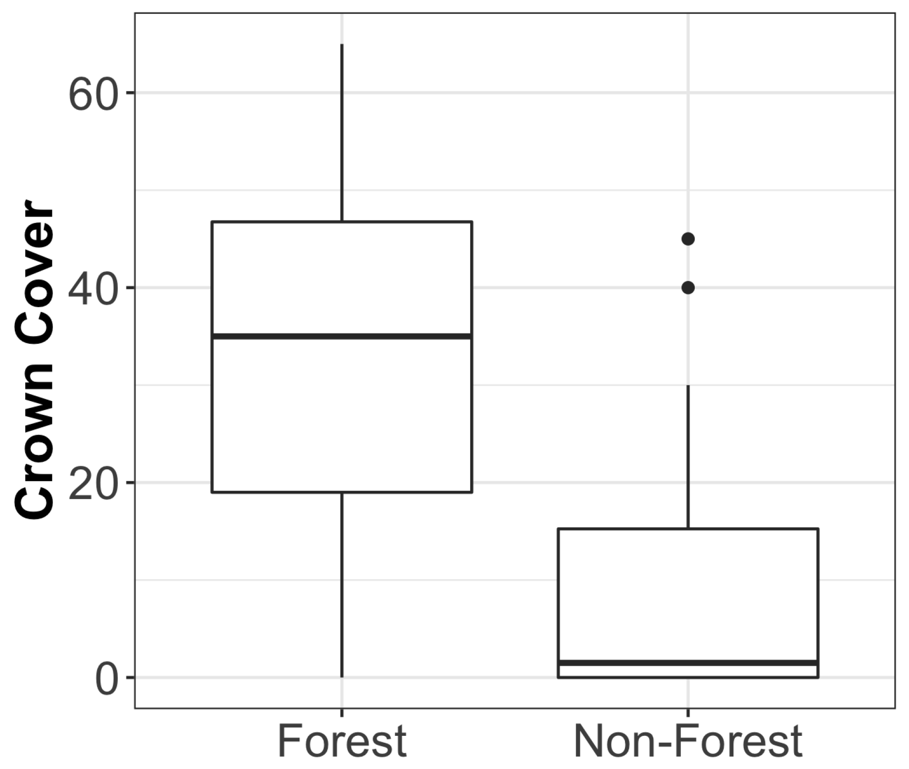
Suppose one categorical auxiliary data product is available. For example, some of the FIA regional units create a map of the population where each population unit is classified into either a forest stratum or a nonforest stratum. A graph of the percent crown cover by stratum is given in Figure 1. Forest classification is a good predictor of canopy cover for Daggett county since most of the plots labeled forest have a larger percent canopy cover than those labeled nonforest. Thus, including this variable in the estimation procedure should decrease the estimator’s variance.

To incorporate a categorical variable with D categories, the variable can be expressed in the linear model using indicator variables, where $x_{ij}=I\{i\in \mathrm{Category} j\}$ for $j=1,2,\dots ,D$. In this case, the model given in Equation (2) reduces to the group mean model,

$$\begin{array}{cc}\hfill y_i& =\sum _{j=1}^D{\beta }_j{x}_{ij}+{ϵ}_i\hfill \end{array}$$

where the intercept term is dropped [46]. Under this model, it is common to assume the variance is constant across the categories, ${\sigma }^2$. The jth entry in the estimated coefficient vector, given Equation (3), reduces to the following stratum mean estimator of y for category j,

$${\hat{\mathit{\beta }}}_{sj}=\frac{1}{n_j}\sum _{i\in s_j}{y}_i={\tilde{\mu }}_{y_j},$$

where $s_j$ represents the sample units in category j and $n_j={\sum }_{i\in s}{x}_{ij}$, the sample size in category j [46]. Now the GREG, given in Equation (1), simplifies to a weighted average of the post-strata means

$$\begin{array}{cc}\hfill {\hat{\mu }}_{y,PS}=& \frac{1}{N}\sum _{j=1}^D\frac{N_j}{n_j}\sum _{i\in s_j}{y}_i=\frac{1}{N}\sum _{j=1}^D{N}_j{\tilde{\mu }}_{y_j},\hfill \end{array}$$

which is the post-stratified estimator (PS). Therefore, the post-stratified estimator is a GREG under a group mean model.

Although here we describe building the post-stratified estimator based on a single categorical variable, the strata can be created by binning a mix of quantitative and categorical variables. McConville and Toth [49] explore the theoretical properties of a post-stratified estimator where the bins are created by a regression tree. In the context of forest inventory, Pulkkinen et al. [50] and Myllymäki et al. [51] explore the utility of post-strata generated by regression trees.

3.2.2. Ratio Estimator

If the available auxiliary variable is quantitative instead of categorical, then a simple model to consider is the ratio model

$$\begin{array}{cc}\hfill y_i& =\beta x_i+{ϵ}_i.\hfill \end{array}$$

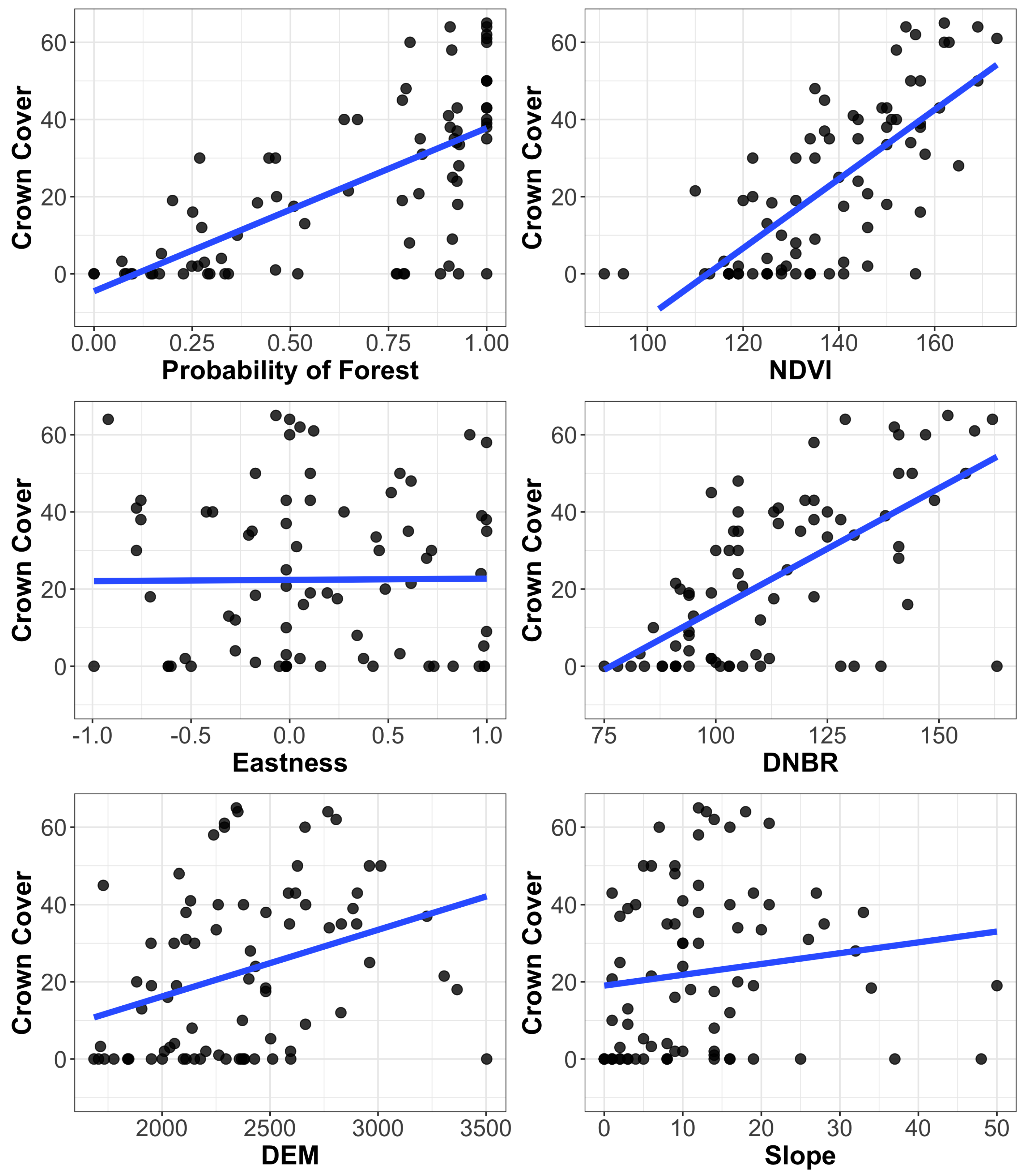
which assumes a linear relationship through the origin. The pairwise scatterplots in Figure 2 allow us to assess the applicability of using this model to approximate the relationship between percent crown cover, one of the variables of interest, and the quantitative auxiliary variables. While several variables appear to have a fairly linear relationship with crown cover, only the relationship between probability of forest and percent crown cover appears to go through, or at least close to, the origin. A common variance structure for the ratio model is ${\sigma }^2{x}_i$. This variance structure is appropriate for the given example since crown cover tends to be more variable as the probability of forest increases.

For the ratio model with ${\sigma }_i^2={\sigma }^2{x}_i$, the estimated coefficient is a ratio of the Horvitz–Thompson estimator of ${\mu }_y$ and the Horvitz–Thompson estimator of ${\mu }_x$,

$${\hat{\beta }}_s={\hat{\mu }}_{x,HT}^{-1}{\hat{\mu }}_{y,HT}$$

and the GREG, given in Equation (1), reduces to [46]

$$\begin{array}{cc}\hfill {\hat{\mu }}_y& =\frac{{\mu }_x}{{\hat{\mu }}_{x,HT}}{\hat{\mu }}_{y,HT}.\hfill \end{array}$$

It is called the ratio estimator (RATIO) because it equals a scaled Horvitz–Thompson estimator where the adjustment term is the ratio of mean value of the auxiliary variable and its corresponding Horvitz–Thompson estimate. While the ratio estimator is simple and can be appropriate when the trend between the variables is a positive, linear relationship through the origin, a REG with a simple linear regression model is usually preferred as it is not constrained by an intercept term set to zero and captures negative linear relationships.

3.2.3. Lasso/Ridge

FIA has access to many more than just a single, auxiliary data product. Thus, consideration of the general linear model is appropriate, but utilizing all of the available predictor variables in the model, along with interaction and higher order terms, can increase the variance of the GREG [7]. Therefore, building the GREG based on a subset of the variables is advantageous. Of course, determining which subset is most appropriate for each variable of interest can be extremely time-consuming. Särndal, Swensson, and Wretman [46] call this factor the “cost of the ‘informed expert’ ” and for inventories such as FIA where there are many y variables, the cost of utilizing an ‘informed expert’ to select a subset of predictor variables for each y can be quite high. In the forest inventory context, Moser et al. [24] explored model selection techniques based on genetic algorithms and random forests. In this paper, we tackle model selection with a penalized regression algorithm where model selection is folded into the estimation of the regression coefficients. This estimation procedure is achieved by adding a penalization to the coefficient estimation criterion which shrinks the magnitude of the coefficients towards zero. Model selection occurs when a subset of the coefficients receives an estimate of zero.

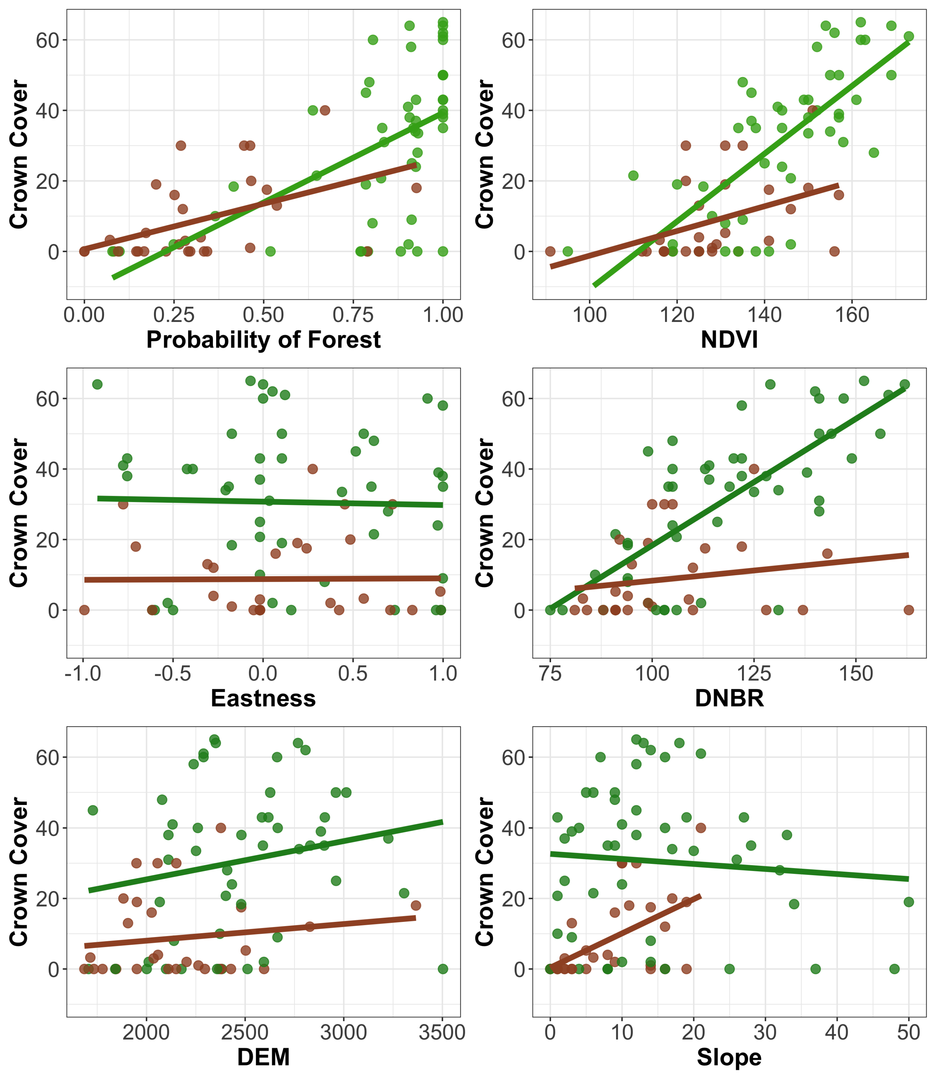
To motivate penalized regression, consider the graphs given in Figure 3. Based on these graphs, a few assessments can be made regarding the utility of the auxiliary variables in the linear regression model. Eastness probably is not a useful predictor of crown cover. In addition, while there appears to be linear relationships, of varying degrees, between crown cover and the other variables, there are also important interactive effects between a couple of the variables and forest classification. 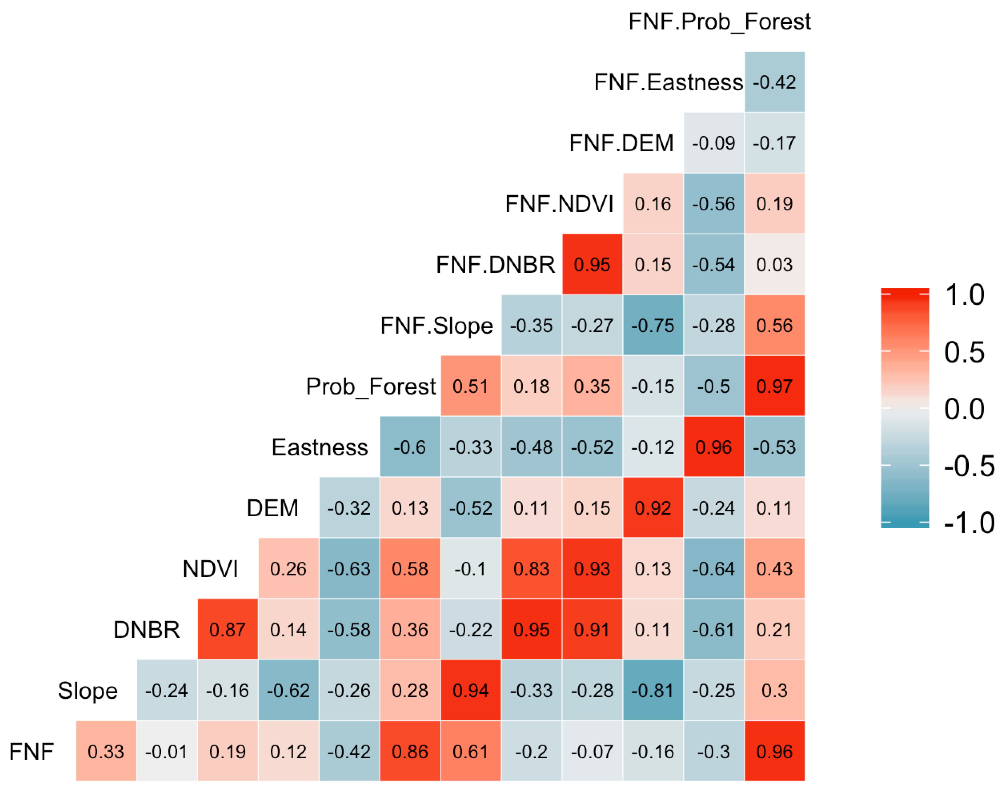Figure 4 provides the pairwise correlations for all seven predictors and their interaction term with FNF. There is a moderately high degree of positive correlation betwen NDVI and DNBR and, as expected, there is a high correlation between the predictors and their interaction term with FNF. These figures imply that both multicollinearity and extraneous predictors exist and therefore a full unpenalized model for crown cover is not advisable.

Instead of using diagnostic graphs to determine the model form, we can consider a large model and incorporate model selection into the coefficient estimation through a penalized least squares criterion. This new criterion, called the elastic net [30], is given by

$$\begin{array}{cc}\hfill {\hat{\mathit{\beta }}}_s& =\underset{\mathit{\beta }}{\arg \min }\left\{\sum _{i\in s}\frac{{(y_i-{\mathit{x}}_i^T\mathit{\beta })}^2}{{\sigma }_i^2}+\lambda \left[\alpha \sum _{j=1}^p\left|{\beta }_j\right|+(1-\alpha )\sum _{j=1}^p{\beta }_j^2\right]\right\}\hfill \end{array}$$

where $\lambda$, a non-negative constant, controls the degree of penalization and $\alpha$, which takes on values between 0 and 1, dictates the mixture of the two different penalties on the coefficients. The first penalty, called the lasso penalty [28], controls the size of the sum of the absolute value of the coefficients and the second penalty, called the ridge penalty [29], controls the size of the sum of the squared coefficients. While both penalties shrink the coefficients towards zero, the lasso penalty will shrink some coefficients to exactly zero if $\lambda$ is large enough. Therefore, the lasso penalty incorporates model selection into the coefficient estimation criterion. However, when multicollinearity is high between predictors, the lasso will tend to only select one of the correlated variables [30]. In these cases of high multicollinearity, the ridge penalty tends to have greater predictive performance [28]. In general, Tibshirani [28] found that the lasso penalty outperforms the ridge penalty when several extraneous auxiliary variables are present and either a few very predictive auxiliary variables or a small to moderate number of moderately predictive auxiliary variables. In contrast, the ridge performs better than the lasso when most of the auxiliary predictors are weakly predictive or multicollinearity is high. If both multicollinearity exists between predictors and several predictors may be extraneous, then elastic net, a compromise between lasso and ridge, is advisable.

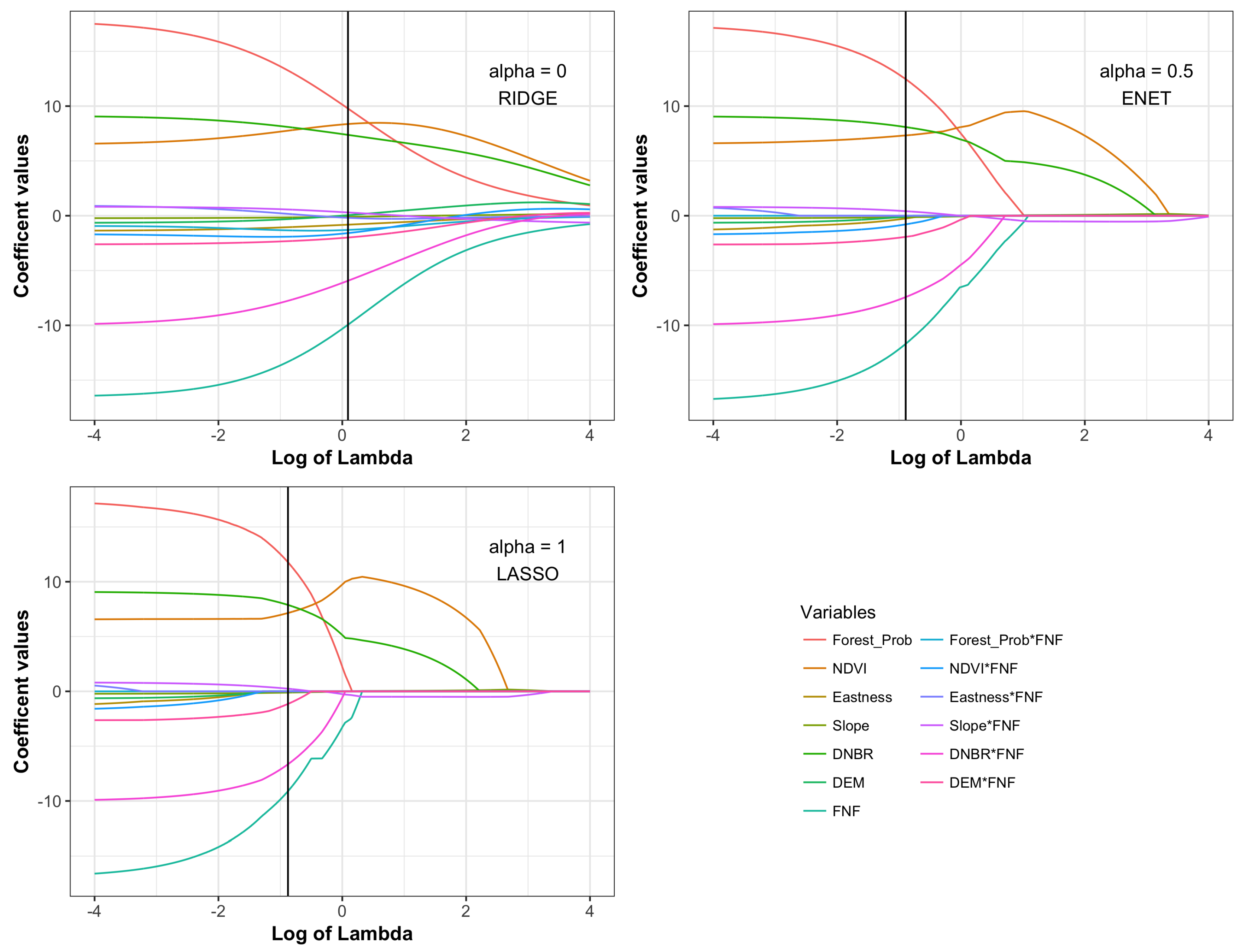
Figure 5 displays the coefficient paths of the model for percent crown cover across a range of $\lambda$ values and for three different penalty mixtures: $\alpha =0,0.5,1$, which we denote by RIDGE, ENET, and LASSO, respectively. As $\lambda$ increases, the coefficient estimates shrink toward zero, though never equaling zero for RIDGE. The selected $\lambda$ value, denoted by the vertical black line in the graphs, is the value which minimizes the mean cross-validation error for 10-fold cross-validation. Three predictors and five predictors were dropped from the model for ENET and LASSO, respectively. While we consider three values for $\alpha$ here, it is also possible to use cross-validation to simultaneously select both $\lambda$ and $\alpha$.

3.3. Estimating the Proportion of a Categorical Variable

For categorical variables, such as presence/absence of a particular species of tree, a common population quantity of interest is the frequency distribution of the variable. We restrict our attention to binary variables, but the results can easily be extended. Let $y_i=I\{i\in \mathrm{category}1\}$ be an indicator function for category 1. Then, ${\mu }_y$ represents the population proportion for category 1.

The REG, along with the specific cases discussed in the previous sub-section, is often employed to estimate ${\mu }_y$. A more realistic working model to assume is the logistic model, which produces estimated proportions that are bounded between 0 and 1. Since the logistic model respects the range of the variable of interest while the linear model does not, a GREG that employs the logistic model has the potential for greater reductions in the variance of the estimator.

In this case, we model the probability the i-th unit is in category 1, given the auxiliary data, with the following formula

$$\begin{array}{c}\hfill P(y_i=1|{\mathit{x}}_i)=\frac{\exp \left({\mathit{x}}_i^T\mathit{\beta }\right)}{1+\exp \left({\mathit{x}}_i^T\mathit{\beta }\right)}=g\left({\mathit{x}}_i^T\mathit{\beta }\right)\end{array}$$

with the logit link function

$$\begin{array}{c}\hfill \mathrm{logit}\left(g\left({\mathit{x}}_i^T\mathit{\beta }\right)\right)=\log \left(\frac{g\left({\mathit{x}}_i^T\mathit{\beta }\right)}{1-g\left({\mathit{x}}_i^T\mathit{\beta }\right)}\right)={\mathit{x}}_i^T\mathit{\beta }.\end{array}$$

The coefficient estimates are found by minimizing the negative log-likelihood under a Bernoulli model:

$$\begin{array}{cc}\hfill {\hat{\mathit{\beta }}}_s& =\underset{\mathit{\beta }}{\arg \min }[-{\displaystyle \sum _{i\in s}}\left\{y_i{\mathit{x}}_i^T\mathit{\beta }-\log \left[1+\exp ({\mathit{x}}_i^T\mathit{\beta })\right]\right\}].\hfill \end{array}$$

The GREG under a logistic model, denoted by LREG, is found by setting $\hat{m}\left({\mathit{x}}_i\right)=g\left({\mathit{x}}_i^T{\hat{\mathit{\beta }}}_s\right)$ in Equation (1) [6]. Model selection is also appropriate under a logistic model and the elastic net (LENET), lasso (LLASSO), or ridge (LRIDGE) penalization can be added to the criterion for the logistic regression coefficient estimates.

3.4. Variance Estimation

From the design-based perspective, the variance of a finite population estimator can be described as a measure of how much the estimate changes from sample to sample under the sampling design, $p(·)$. The formula for the variance is given by

$$V_p\left({\hat{\mu }}_y\right)=E_p\left\{{\left[{\hat{\mu }}_y-E_p\left({\hat{\mu }}_y\right)\right]}^2\right\}$$

with design expected value $E_p\left({\hat{\mu }}_y\right)={\sum }_{s\subset U}{\hat{\mu }}_y\left(s\right)p\left(s\right)$. The variance of the HT is given by

$$\begin{array}{c}\hfill V\left({\hat{\mu }}_{y,HT}\right)=\left(1-\frac{n}{N}\right)\frac{1}{n}\frac{1}{N-1}\sum _{i\in U}{\left(y_i-{\mu }_y\right)}^2\end{array}$$

where an unbiased estimator is obtained by replacing the population variance with the sample variance [46]

$$\begin{array}{c}\hfill \hat{\mathrm{V}}\left({\hat{\mu }}_{y,HT}\right)=\left(1-\frac{n}{N}\right)\frac{1}{n}\frac{1}{n-1}\sum _{i\in s}{\left(y_i-{\hat{\mu }}_{y,HT}\right)}^2.\end{array}$$

Since the GREG is a complex function of the sample, the variance of the GREG cannot be written in a closed form. Using a Taylor expansion of ${\hat{\mu }}_y$, one can obtain an approximate variance

$$\begin{array}{c}\hfill \mathrm{AV}\left({\hat{\mu }}_y\right)=\left(1-\frac{n}{N}\right)\frac{1}{n}\frac{1}{N-1}\sum _{i\in U}{\left(y_i-m_U\left({\mathit{x}}_i\right)\right)}^2\end{array}$$

(4)

where $m_U(·)$ is the population-level fit of the model. While $\mathrm{AV}\left({\hat{\mu }}_y\right)$ tends to approximate the true variance well for models with few predictors, it can underestimate the true variance as the model size grows since Equation (4) does not include a term that captures model estimation error. Notice from the form of Equation (4) that the approximate variance can only decrease as more predictors are added to the model. However, the true variance may increase since the model fits become more variable.

The approximate variance cannot be computed since it depends on population values for both $\mathit{x}$, which are known, and y, which are unknown outside of the sample. The utility of the approximate variance is that it provides a variance estimator formula to modify with sample-based components. The standard method to estimate the variance is to plug the sample estimated model prediction, $\hat{m}(·)$, in for the population-level fit of the model, $m_U(·)$, and to average the squared residual terms over the sample (instead of the population),

$$\hat{V}\left({\hat{\mu }}_y\right)=\left(1-\frac{n}{N}\right)\frac{1}{n}\frac{1}{n-1}\sum _{i\in s}{\left(y_i-\hat{m}\left({\mathit{x}}_i\right)\right)}^2.$$

This estimator is asymptotically unbiased for the GREG under mild regularity conditions [52]. The standard variance estimator does, however, have some shortcomings for finite samples. The estimator tends to underestimate the true variance for large working models since it does not account for the estimation error in $\hat{m}\left(\mathit{x}\right)$ [48]. Similar to the approximate variance, the variance estimator will only decrease as predictors are added to the working model; however, the true variance may actually increase, especially if the number of predictors is large compared to the sample size. McConville et al. [7] show that, as the number of predictors in the working model increases, the negative bias of the standard variance estimator also increases. Beyond parametric working models, Kangas et al. [14] provide evidence that the standard variance estimator can also underestimate the variance when a kernel model is employed as the working model.

One alternative is to construct a bootstrap variance estimator which captures the estimate’s sampling variability if the bootstrap procedure correctly mimics the sampling procedure. In this paper, we focus on the bootstrap procedure under simple random sampling without replacement. See Mashreghi, Haziza, and Léger [53] for bootstrap methods which handle other complex sampling designs.

The bootstrap method mimics the variability induced by the sampling design by taking a random sample with replacement from the sample. The steps of the bootstrap procedure are:

• Take a simple random sample with replacement of size n from the original sample. Since you are sampling with replacement, you won’t get the same sample back each time. This sample is called a bootstrap sample.
• Compute the estimator, ${\hat{\mu }}_y$, on the bootstrap sample.
• Repeat step 1 and step 2 $B-1$ more times until the mean of the bootstrap estimates and the standard error of the bootstrap estimates have satisfied a convergence criterion, such as there is less than a one percent change in the mean and standard error over all iterations compared to the mean and standard error for the first $B-100$ iterations.

The bootstrap variance estimator is given by

$${\hat{V}}_B\left({\hat{\mu }}_y\right)=\left(\frac{n}{n-1}\right)\left(\frac{N-n}{N-1}\right)\frac{1}{B-1}\sum _{b=1}^B{({\hat{\mu }}_y^{\left(b\right)}-{\overline{\hat{\mu }}}_y)}^2$$

where ${\hat{\mu }}_y^{\left(b\right)}$ is the bth bootstrap estimate and ${\overline{\hat{\mu }}}_y=B^{-1}{\sum }_{b=1}^B{\hat{\mu }}_y^{\left(b\right)}$. The bootstrap variance estimator has two bias adjustment terms: $n{(n-1)}^{-1}$ adjusts for the bias induced by taking a bootstrap sample (i.e., sampling with replacement from the sample) instead of a random sample from the population and $(N-n){(N-1)}^{-1}$ accounts for the without replacement sampling in the original design. In Section 5, we conduct a simulation study to compare the performance of the standard variance estimator and the bootstrap variance estimator for the GREGs presented in this article.

3.5. Survey Weights

For a particular variable of interest, we have focused on finding which form of the GREG and which subset of predictors provides an estimate with a small standard error. That is, we have given examples in specific inference. However, FIA reports on many characteristics of forest ecosystems. In this case, it is not feasible to specify a unique working model for each variable. Instead, generic inference is employed where a single set of survey weights is applied to all variables of interest to produce the necessary estimates. Survey weights are derived from our sampling design and adjusted based on our ancillary information to ensure internal consistency amongst the estimates.

Fortunately, all of the linear regression estimators, except the LASSO and ENET, can be written as a weighted average of the variable:

$$\begin{array}{c}\hfill {\hat{\mu }}_y=N^{-1}\sum _{i\in s}{w}_i{y}_i\end{array}$$

(5)

where ${\left\{w_i\right\}}_{i\in s}$ is the set of survey weights. In particular, the REG estimator can be written as

$${\hat{\mu }}_y=N^{-1}\sum _{i\in s}\left[1+N{({\mathit{\mu }}_x-{\hat{\mathit{\mu }}}_{x,HT})}^T{\left(\sum _{j\in s}\frac{{\mathit{x}}_j{\mathit{x}}_j^T}{{\sigma }_j^2}\right)}^{-1}{\mathit{x}}_i\right]y_i=N^{-1}\sum _{i\in s}{w}_i{y}_i$$

where ${\mathit{\mu }}_x$ is a vector that contains the finite population means of the auxiliary variables and ${\hat{\mathit{\mu }}}_{x,HT}$ contains the corresponding HT estimators. The LASSO, ENET, and GREG estimators that employ a logistic or penalized logistic model can not be written in this form because the model fits of these estimators are not linear combinations of the y-values.

Notice that the survey weights are a function of the auxiliary data and inclusion probabilities and are not a function of the variable of interest itself. This implies that the survey weights can be applied to any variable of interest to obtain a mean estimator of the desired attribute. However, the variance of the estimator will still depend on how well the linear model and set of variables predict the variable of interest. Therefore, it is important to pick a set of auxiliary variables that relate with a broad number of the forest variables when conducting generic inference.

3.5.1. Condition-Level Estimates

The linearity of Equation (5) allows the estimator to be broken down by condition or by domain. A condition is defined as an area of relatively uniform ground cover, such as water, nonforest, or forest, further partitioned by forest type, stand size class, regeneration status or tree density and a domain is a sub-population, such as county, of the finite population of interest. An important distinction between conditions and domains is that a plot can be partitioned by multiple conditions while it only belongs to a single domain.

Suppose there are K possible conditions. Let $c_{ik}$ be the proportion of plot i that is in condition k and note that ${\sum }_{k=1}^K{c}_{ik}=1$. In this case, the population total of variable y in condition k is given by $t_{y,c_k}={\sum }_{i\in U}{y}_i{c}_{ik}$ and is estimated by applying the survey weights to the set ${\left\{y_i{c}_{ik}\right\}}_{i\in s}$, ${\hat{t}}_{y,c_k}={\sum }_{i\in s}{w}_i{y}_i{c}_{ik}$. An important property is that the sum of the total estimates across conditions equals the estimate of the sum of the totals across conditions:

$$\begin{array}{cc}\hfill {\hat{\mu }}_y& =N^{-1}{\hat{t}}_y\hfill \\ \hfill & =N^{-1}{\displaystyle \sum _{i\in s}}{w}_i{y}_i\hfill \\ \hfill & =N^{-1}{\displaystyle \sum _{i\in s}}{w}_i{y}_i(c_{i1}+c_{i2}+\cdots +c_{iK})\hfill \\ \hfill & =N^{-1}\left({\displaystyle \sum _{i\in s}}{w}_i{y}_i{c}_{i1}+{\displaystyle \sum _{i\in s}}{w}_i{y}_i{c}_{i2}+\cdots +{\displaystyle \sum _{i\in s}}{w}_i{y}_i{c}_{iK}\right)\hfill \\ \hfill & =N^{-1}\left({\hat{t}}_{y,c_1}+{\hat{t}}_{y,c_2}+\cdots +{\hat{t}}_{y,c_K}\right),\hfill \end{array}$$

This condition ensures that the estimates in a table will add up to the marginals of the table, a valuable measure of internal consistency.

3.5.2. Domain Estimates

Suppose the finite population can be partitioned into H sub-populations or domains, $U=U_1\cup U_2\cup \dots \cup U_H$ and similarly the sample can be partitioned, $s=s_1\cup s_2\cup \dots \cup s_H$. The total of domain h is $t_{y,h}={\sum }_{i\in U_h}{y}_i$ and the survey weighted domain estimate is ${\hat{t}}_{y,h}={\sum }_{i\in s_h}{w}_i{y}_i$. As with the condition-level estimates, the domain estimates are also internally consistent:

$$\begin{array}{cc}\hfill {\hat{\mu }}_y& =N^{-1}{\displaystyle \sum _{i\in s}}{w}_i{y}_i\hfill \\ \hfill & =N^{-1}{\displaystyle \sum _{i\in s}}{w}_i{y}_i(I\{i\in s_1\}+I\{i\in s_2\}+\cdots +I\{i\in s_H\})\hfill \\ \hfill & =N^{-1}{\displaystyle \sum _{i\in s_1}}{w}_i{y}_i+{\displaystyle \sum _{i\in s_2}}{w}_i{y}_i+\cdots +{\displaystyle \sum _{i\in s_H}}{w}_i{y}_i\hfill \\ \hfill & =N^{-1}\left({\hat{t}}_{y,1}+{\hat{t}}_{y,2}+\cdots +{\hat{t}}_{y,H}\right).\hfill \end{array}$$

This type of domain estimator is called an indirect estimator because the same model is applied across all domains. A direct estimator would allow the model to vary across domains and would produce a set of weights ${\left\{w_i\right\}}_{i\in s_h}$ for each domain.

4. Daggett County Estimates

For the four quantitative variables of interest, percent canopy cover, basal area per hectare, trees per hectare, and volume of trees, estimates of the population mean and bootstrap standard error were computed for each of the estimators presented in Section 2 where constant variance was assumed for each model except the ratio model. In terms of predictors, the HT utilized no auxiliary data, the PS utilized FNF, the RATIO and REG_2 used Prob_Forest, and the other estimators utilized the six quantitative predictors, FNF, and the interactions between the quantitative predictors and FNF. The penalized regression estimators, LASSO, ENET, and RIDGE can be seen as potential compromises between the REG_1 which uses the full model and the REG_2 which uses a simple linear regression model with the generally strongest predictor.

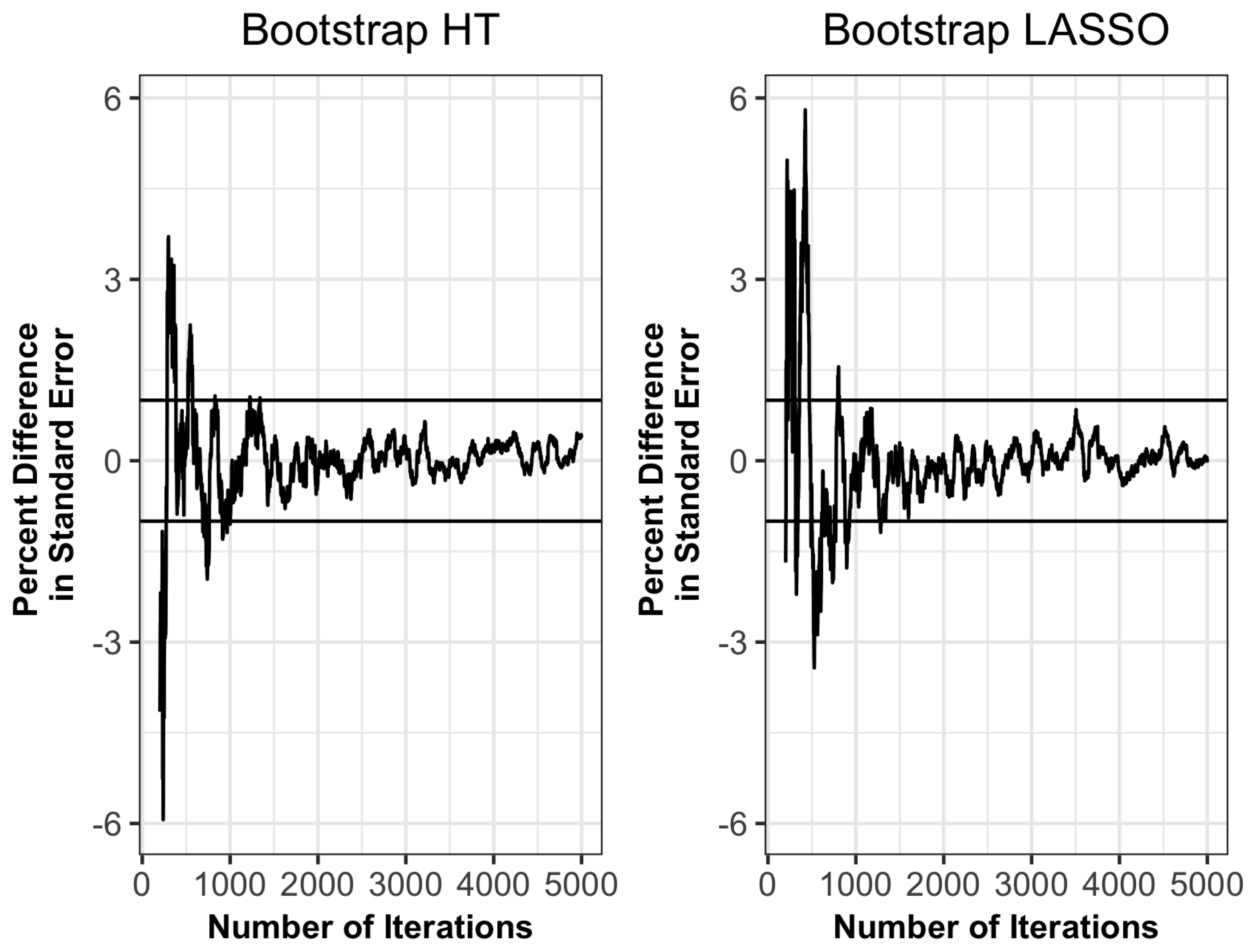
For the four binary variables, presence or absence of lodgepole pine, presence or absence of pinyon-juniper, presence or absence of aspen and forest or non-forest, an estimate of the population proportion and bootstrap standard error were computed, where a logistic regression model was used for the LREG_1, LREG_2, LLASSO, LENET, and LRIDGE and the same predictors were utilized as those used for the quantitative variables of interest. For each estimator, 5000 bootstrap samples were taken to compute the bootstrap standard error, although the standard error estimates tended to consistently meet the convergence rule after 2000 iterations as shown in Figure A1 in the Appendix A.

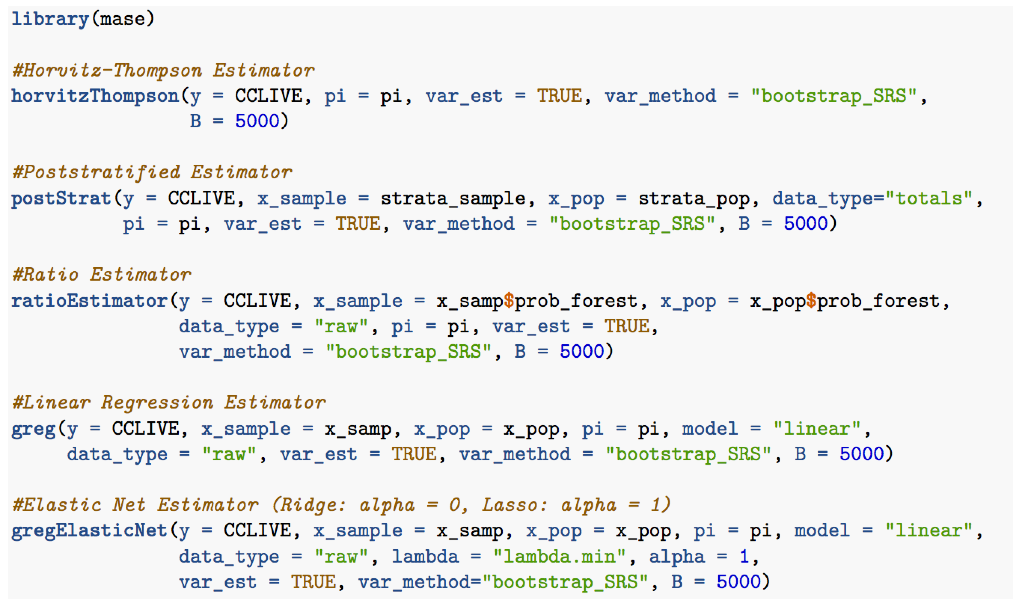
The estimates and the relative standard errors for the quantitative variables are given in

Table 1. Mean estimates (Estimate) and relative standard errors (RSE) for the quantitative forest variables.

	Canopy Cover		Basal Area (per Hectare)		Trees (per Hectare)		Volume (Cubic Meters per Hectare)
Estimator	Estimate	RSE	Estimate	RSE	Estimate	RSE	Estimate	RSE
HT	22.43	10.48	157.61	11.92	809.92	17.96	42.64	12.17
PS	22.89	8.74	159.59	11.37	831.15	16.30	43.62	10.25
RATIO	21.23	7.91	149.19	10.69	766.66	16.01	40.36	9.86
REG_1	23.46	7.72	160.06	15.21	768.46	13.87	41.37	12.01
REG_2	20.99	8.05	149.60	11.09	740.23	15.08	39.80	9.87
LASSO	23.38	6.84	162.26	12.01	784.36	13.85	42.79	10.38
ENET	23.63	6.73	164.82	11.76	838.11	13.35	42.94	10.11
RIDGE	23.51	6.59	161.07	12.97	787.13	13.53	41.89	10.29

and

Table 2. Proportion estimates (Estimate) and relative standard errors (RSE) for the categorical forest variables.

	Lodgepole Pine		Pinyon-Juniper		Aspen		Forest
Estimator	Estimate	RSE	Estimate	RSE	Estimate	RSE	Estimate	RSE
HT	0.24	19.75	0.30	17.33	0.14	28.26	0.74	6.78
PS	0.25	17.89	0.30	17.39	0.14	26.76	0.75	5.63
RATIO	0.22	17.78	0.28	17.61	0.13	26.92	0.70	5.16
LREG_1	0.26	10.55	0.30	15.46	0.17	33.53	0.71	7.30
LREG_2	0.20	15.35	0.30	17.57	0.12	26.83	0.72	5.29
LLASSO	0.28	11.87	0.30	14.86	0.15	26.85	0.72	5.39
LENET	0.26	13.69	0.29	14.98	0.14	27.54	0.73	5.73
LRIDGE	0.27	11.85	0.29	14.73	0.14	27.59	0.72	5.26

for the binary variables. All estimates and their relative standard errors were generated using the mase package [31] in R [54]. Example code for generating estimates for quantitative and binary variables using the regression estimator is displayed in Figure 6.

Several observations can be made about the estimators and the relative performance of the estimators. Because the proportion of forested land in U happens to be greater than the proportion in this particular sample, the PS tends to yield slightly larger estimates than the HT. The PS also yields a smaller standard error than the HT, providing evidence that this simple forest indicator is a useful predictor for many forest variables. However, the RATIO and REG_2/LREG_2, which utilize the quantitative variable, Prob_Forest, instead of the forest indicator variable, provide further gains in performance and produce estimates that are smaller than HT or PS. For this example, the quantitative variable Prob_Forest is a stronger predictor than the categorical variable FNF and therefore the PS has a higher SE. For situations where the strongest predictor is categorical, the PS will likely have a smaller standard error than the RATIO or REG_2/LREG_2.

Recall that the RATIO is most appropriate when you have access to one quantitative auxiliary variable and want to utilize regression through the origin. Another option when you have a single quantitative variable is to fit the REG or LREG, which utilize simple linear regression or logistic regression, respectively. These estimates are given by REG_2 and LREG_2 in our results. As seen in the results the RATIO and REG_2/LREG_2 perform fairly similarly but the REG_2/LREG_2 is more flexible since it allows for an intercept term in the model.

The HT and PS tend to be more variable than the REG_1 and LREG_1, which use all of the predictors in a linear and a logistic model, respectively. However, the standard error of the REG_2 and LREG_2 can be negatively impacted by a large model, as observed in estimating the average basal area per tree or the average canopy cover. In both of these cases, the RATIO and REG_2 outperform the REG_1 because they were built using only the most useful variable. This comparison showcases the importance of selecting a good subset of predictors for the estimators, a feature of the penalized techniques. The penalized regression estimators are fairly similar in their sampling variability and have the smallest standard error for most of the forest variables.

These results also provide insights into the challenges of generic inference. PS can be seen as a simple generic estimator while REG_1 is a more complex generic estimator but both have their drawbacks. If we construct a single set of weights based on PS, then we lose precision in estimating attributes such as average trees per hectare, which correlates with most of the auxiliary variables, resulting in 10 out of 13 non-zero coefficients in the LASSO estimator. However, if we instead use all of the auxiliary variables as REG_1 does, then we lose efficiency when estimating attributes that don’t relate with most of the auxiliary variables. For example, the LASSO estimator for the presence of aspen only retained 3 of the 13 model coefficients and its LREG_1 had the highest relative standard error. Selecting a good set of variables for creating generic survey weights requires balancing the gains in precision from estimating attributes that relate with the auxiliary data and the losses for attributes that are uncorrelated with the auxiliary data.

5. Simulation Study

To further illustrate the relative performance of the estimators and variance estimators presented, we report the results of a simulation study. In particular, we study the impact of including irrelevant auxiliary information when fitting the working model, $m\left(\mathit{x}\right)$. Since model-assisted estimators are robust, in terms of bias, to model mis-specification, we sought to understand how much the inclusion of irrelevant variables increases the variance of the estimator and impacts the variance estimators.

We consider the following model for generating the variable of interest:

$$y_i=2x_{1i}+0.5x_{2i}+0x_{3i}+\cdots +0x_{pi}+{ϵ}_i$$

where ${ϵ}_i$ follows a shifted exponential distribution with mean of zero and the rate parameter, which describes the distribution’s shape, of 0.2. Therefore, the model contains two relevant predictor variables and $p-2$ irrelevant predictor variables. Each auxiliary variable, $x_j$, is generated independently from a normal distribution with a mean of six and a standard deviation of 2 except $x_3$ and $x_4$. These variables were generated to have a correlation of 0.89 and 0.71 with $x_2$ to make it more difficult for the lasso method to detect whether or not these predictors are relevant. To study the impact of irrelevant predictors and of the working model size, we let the number of auxiliary variables to grow, setting p equal to $10,20,40$ when fitting the REG, LASSO, and RIDGE. We compare these estimators to the oracle estimator (ORACLE), a REG built with the true predictors, $x_1$ and $x_2$. While the ORACLE is infeasible in practice, in simulations, it allows us to study the impact of irrelevant predictors. Since the useful predictors are quantitative, not categorical, we excluded PS from the simulation study. We also excluded the ENET because it behaved very similarly to the LASSO.

We generated a single finite population of size N = 10,000. We then drew 2000 simple random samples of size $n=150$ with replacement. We chose a sample size of 150 because this is typical number of ground plots in a county in the Interior West. The repeated sampling from a single population mimics the expected variability of the sampling design and therefore allows us to compute the empirical mean,

$$\mathrm{E}\left({\hat{\mu }}_y\right)=\frac{1}{1000}\sum _{b=1}^{1000}{\hat{\mu }}_y^{\left(b\right)},$$

the empirical variance,

$$\mathrm{Var}\left({\hat{\mu }}_y\right)=\frac{1}{1000}\sum _{b=1}^{1000}{\left[{\hat{\mu }}_y^{\left(b\right)}-\mathrm{E}\left({\hat{\mu }}_y\right)\right]}^2,$$

and the empirical root mean squared error

$$\mathrm{RMSE}\left({\hat{\mu }}_y\right)=\sqrt{\frac{1}{1000}\sum _{b=1}^{1000}{\left[{\hat{\mu }}_y^{\left(b\right)}-{\mu }_y\right]}^2}=\sqrt{\mathrm{Bias}{\left({\hat{\mu }}_y\right)}^2+\mathrm{Var}\left({\hat{\mu }}_y\right)},$$

where ${\hat{\mu }}_y^{\left(b\right)}$ is the value of the estimator for the b-th sample. Although all of the estimators presented are asymptotically unbiased under a wide range of sampling designs, they can still exhibit bias in finite samples. Therefore, we also compute the percent relative bias of the estimator

$$\left[\frac{\mathrm{E}\left({\hat{\mu }}_y\right)-{\mu }_y}{{\mu }_y}\right]100\%=\left[\frac{\mathrm{Bias}\left({\hat{\mu }}_y\right)}{{\mu }_y}\right]100\%.$$

for both the estimators and the variance estimators.

The percent relative bias was less than 1% for all estimators and is therefore not displayed.

Table 3. Simulation Results: Ratio of root mean squared errors compared to ORACLE (Root MSE Ratios), percentage relative bias (PRB) of standard and bootstrap variance estimators, confidence interval (CI) coverage for nominal 95% confidence intervals.

		Empirical Variance	Root MSE Ratios	PRB of Standard Variance Estimators	PRB of Bootstrap Variance Estimators	CI Coverage with Standard Variance Estimators	CI Coverage with Bootstrap Variance Estimators
	HT	0.27	1.30	3.43	3.32	95.70	95.55
	ORACLE	0.16	1.00	−1.04	1.70	94.50	94.95
p = 5	REG	0.16	1.01	−5.27	1.88	93.95	94.95
	LASSO	0.16	1.01	−3.59	0.72	94.20	95.10
	RIDGE	0.16	1.01	−4.42	1.41	94.00	95.20
p = 10	REG	0.17	1.02	−11.44	3.67	92.10	94.25
	LASSO	0.16	1.01	−5.09	0.56	92.65	93.70
	RIDGE	0.17	1.02	−9.44	2.01	92.60	93.85
p = 20	REG	0.19	1.06	−27.11	2.64	89.85	94.75
	LASSO	0.18	1.02	−13.70	−7.75	92.10	92.85
	RIDGE	0.19	1.05	−23.58	−5.64	90.85	93.55
p = 20	REG	0.22	1.17	−46.85	25.42	83.75	96.25
	LASSO	0.16	1.01	−7.50	−0.43	93.30	94.45
	RIDGE	0.19	1.09	−30.31	−3.03	88.60	93.65

displays the empirical variance of the estimators. All estimators are less variable than HT, which uses no working model. However, as the model size increases, so does the variance of the estimator. Since we have access to the entire population, the approximate variance of each estimator, given by Equation (4), was also computed. For HT, the approximate variance was essentially equal to the empirical variance, while for the rest of the estimators the approximate variance was about 0.11, regardless of p. For these estimators, the approximate variance underestimated the true variance, especially as p increased, an issue discussed in Section 3.4.

To compare the efficiency of the estimators, Table 3 also contains the ratio of the root mean squared error of the estimators to the root mean squared error of the ORACLE. As the number of extraneous predictors increases, the REG becomes more variable. The LASSO remains almost as variable as the ORACLE and the RIDGE, which shrinks the coefficient estimates but does not perform model selection, is slightly less efficient than the LASSO.

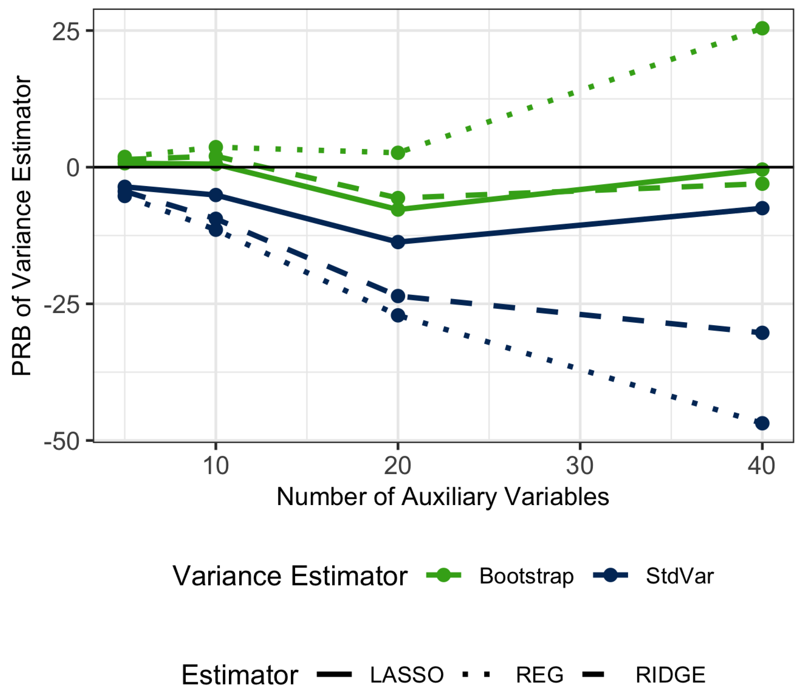
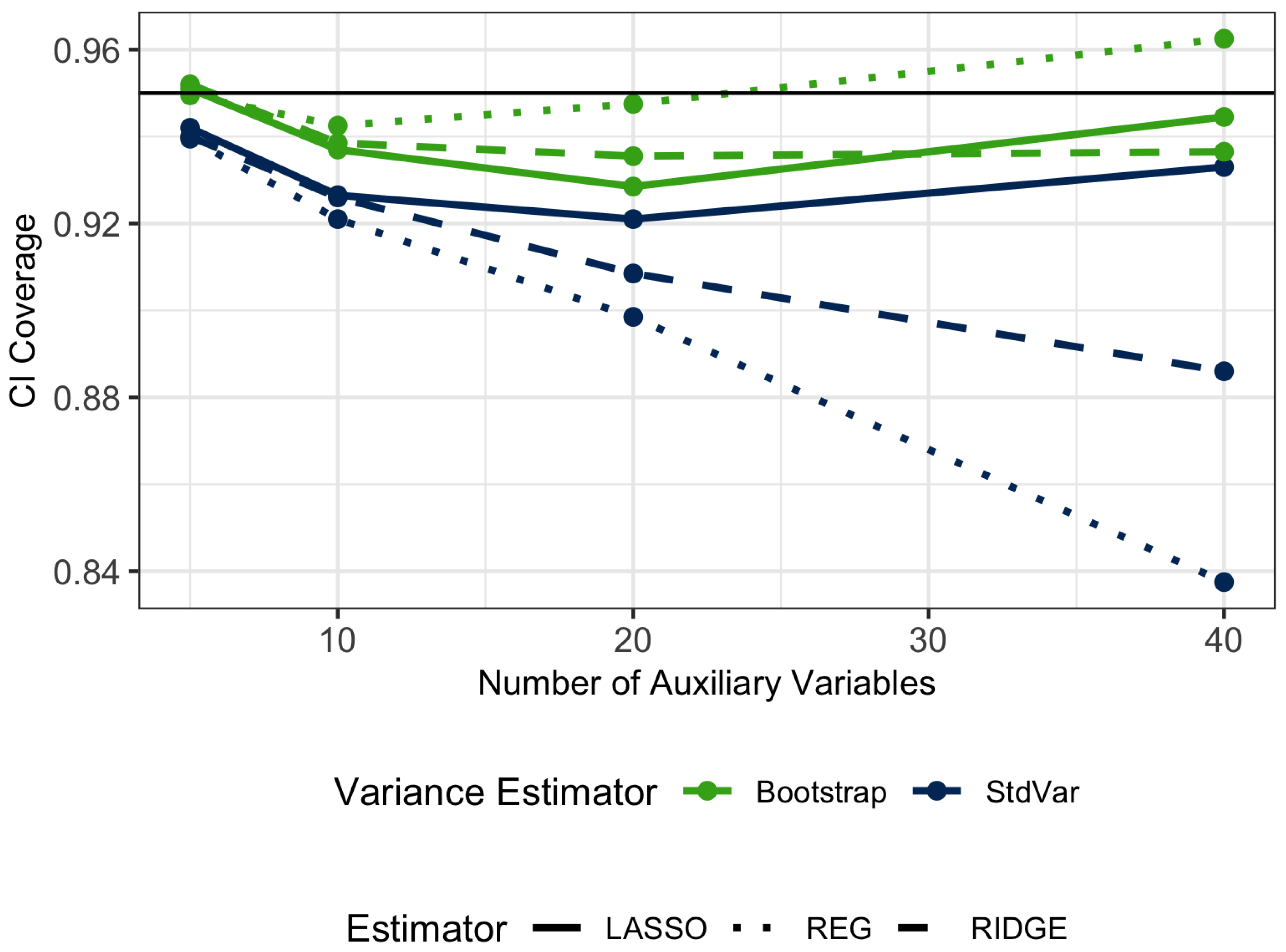
Regarding the variance estimators, Table 3 displays the percent relative bias of the variance estimators and the confidence interval coverage for nominal 95% confidence intervals for all of the estimators. Figure 7 and Figure 8 track the relationship between the number of auxiliary variables and the percent relative bias of the variance estimators and confidence interval coverage. The standard variance estimator has significant negative bias which increases as the models contain more extraneous variables. The bootstrap variance estimator is less biased and produces confidence intervals that are closer to the nominal coverage. The bootstrap variance estimator does overestimate the variance for the REG when the number of predictors is 40, likely since the ratio of sample size to predictors is small in this case and therefore the model fits are highly variable. For the penalized regression estimators, the bootstrap variance estimator stays close to the true variance, even as the number of predictors increases.

6. Conclusions

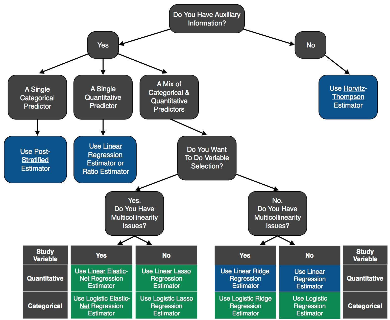
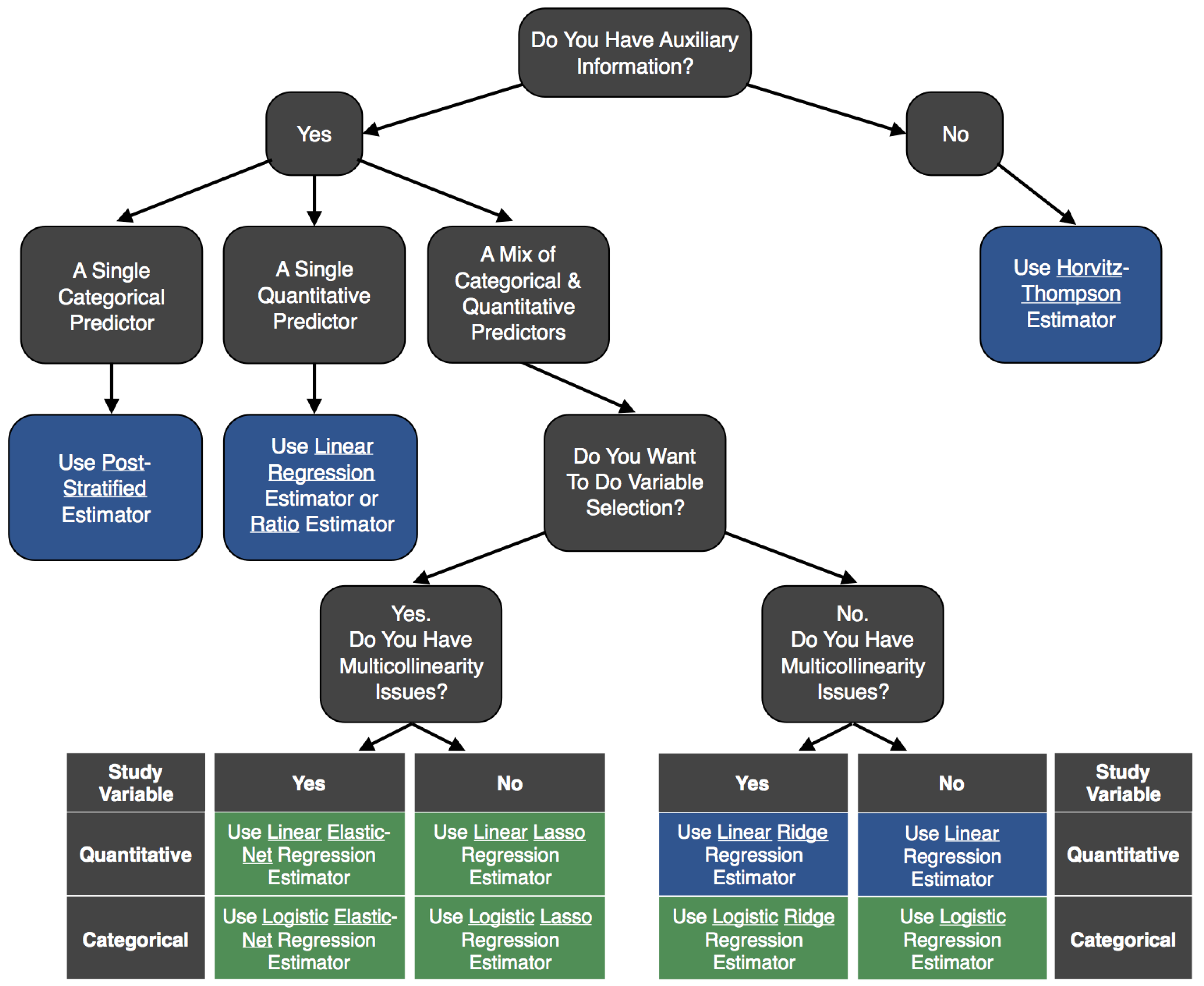
The utility of a given estimator and variance estimator depends on what auxiliary data are available and how the auxiliary data relate with the variable of interest. Figure 9 summarizes the differences between the estimators and their applicability based on the available data. Since the elastic net and lasso perform variable selection, these methods can also help determine which ancillary data layers enhance estimates of forest attributes. Although forest inventories do estimate other population quantities, such as ratios, these quantities can often be written as a function of means. In that case, the quantity can be estimated by inserting the estimated means using one of the model-assisted estimators described in this paper. When estimating a ratio, the resulting estimator would be a ratio of model-assisted estimators. The variance can also be estimated by utilizing the bootstrap procedure given in Section 3.3 where the function of the estimated means is computed at Step 2.

In this paper, we present a class of model-assisted, parametric, generalized regression estimators. By progressively stepping through each estimator, we illustrate how poststratification, ratio, regression, lasso, ridge, and elastic net are all just special cases of a GREG. This allows different estimators to be more easily explained to a broad user community that is currently most familiar with poststratification. We illustrate that all of the linear regression estimators of the population mean, except the lasso and elastic net, can be written in the form of survey weights, and thus support generic inference where means and totals on many forest variables need to be estimated simultaneously. Through simulation, we also illustrate how sensitive closed form variance estimators can be subject to underestimating the variance, building a stronger case for bootstrap variance estimators in practice. The magnitude of the negative bias is difficult to predict since it depends on many factors, including the sample size, the number of auxiliary variables, the correlation structure between the auxiliary variables, and the signal-to-noise ratio. More work is needed to develop specific guidelines for when the standard variance estimator is no longer appropriate, as well as to explore the consequences of assuming a simple random sample design for something that is quasi-systematic. As pointed out by Magnussen et al. [55], when there is a trend in the data, variance estimators based on simple random sampling but applied to a systematic sample will over-estimate the variance. Improvements in variance estimates using a model-assisted estimator with auxiliary data correlated with the trend may be correcting for the over estimation of variances under the simple random sampling assumption, providing a more realistic estimate of the variance. This offers a different perspective on potential benefits of model-assisted estimators in forest inventory applications that warrants further investigation. We have uploaded the user-friendly mase package for immediate use in applications involving any sample survey data. For users of FIA data who need automated database queries and spatial intersection capabilities, mase has been incorporated into the R package FIESTA which is in beta test mode at the time of this publication and slated for public release in the fall.