Parameter Optimization of the 3PG Model Based on Sensitivity Analysis and a Bayesian Method


Abstract
:1. Introduction
2. Materials and Methods
2.1. Study Site
2.2. Methods
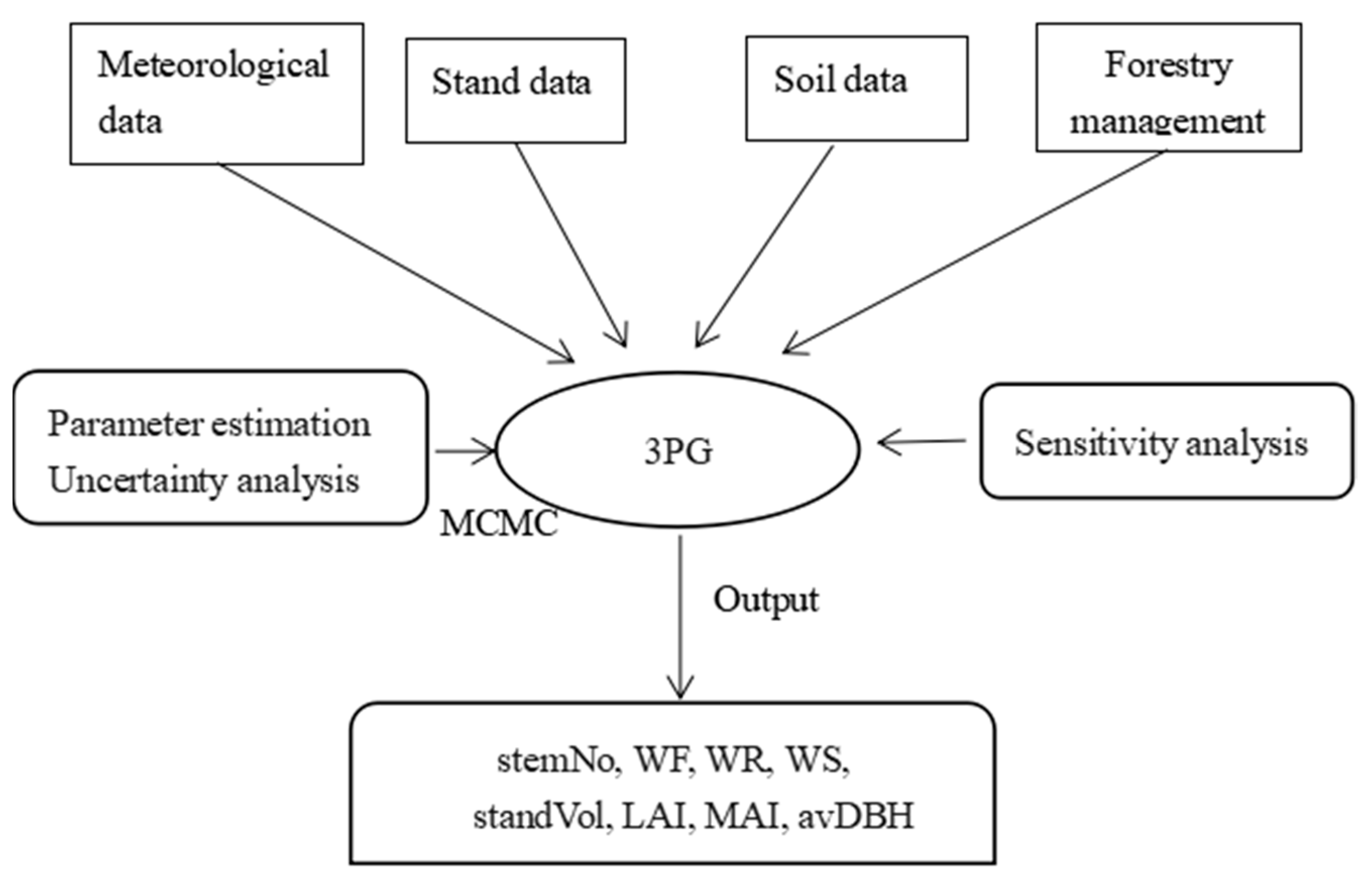
2.2.1. 3PG Model
2.2.2. Sensitivity Analysis
2.2.3. MCMC
3. Results
3.1. 3PG Model
3.2. MCMC Result
3.3. Comparative Analysis
4. Discussion
4.1. Parameter Sensitivity
4.2. Parameter Optimization using MCMC
4.3. Model Uncertainty
5. Conclusions
- (1)
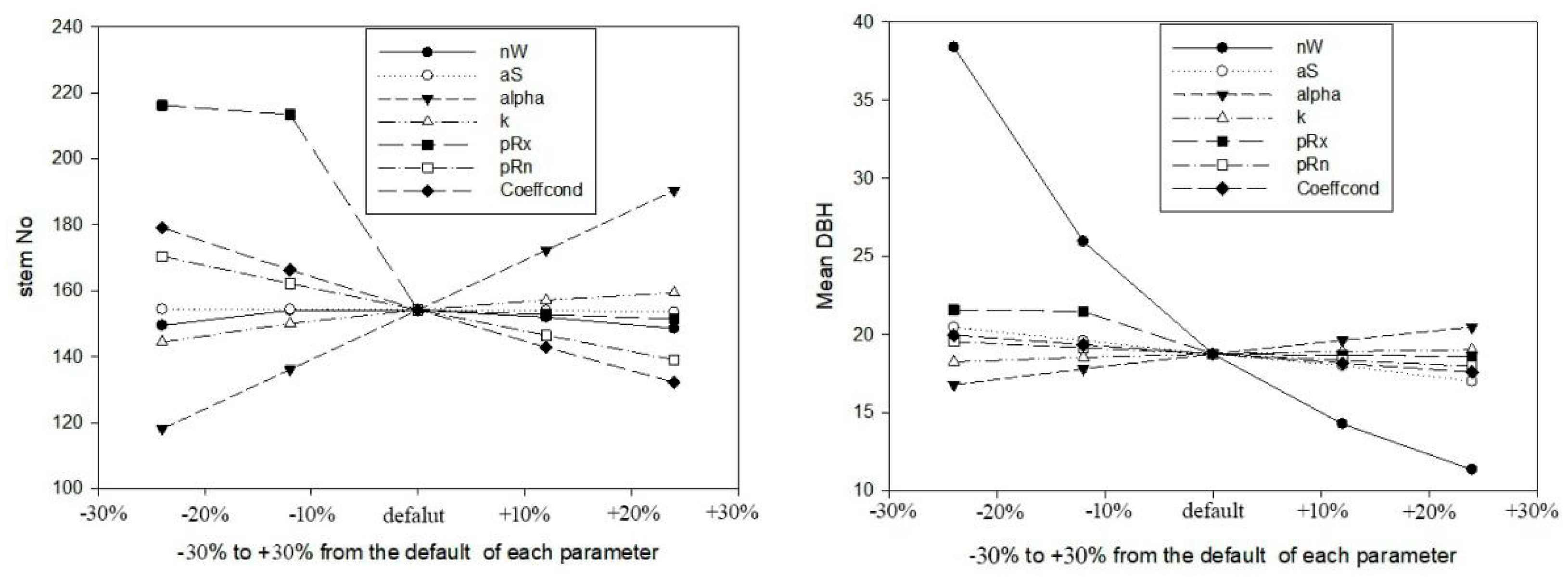
- Among the 63 parameters of the 3PG model, the parameters that are most sensitive to stand stocking and DBH were nWs, aWs, alphaCx, k, pRx, pRn, and CoeffCond.
- (2)
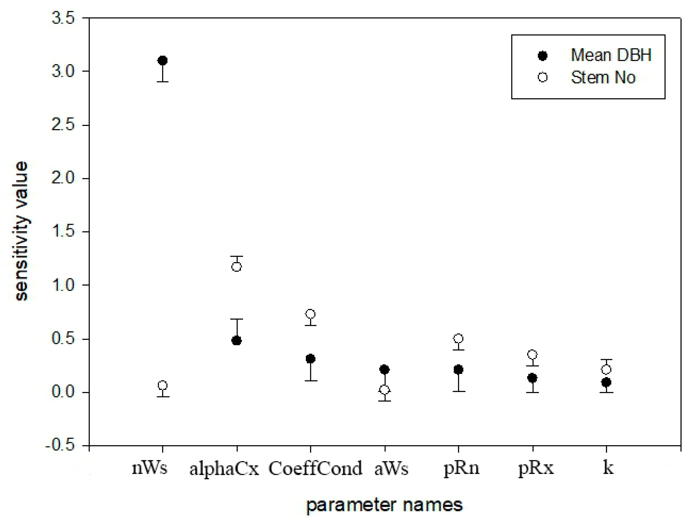
- The parameters that have the greatest influence on stand stocking are alphaCx, CoeffCond, pRn, pRx, k, nWs, and aW, and the parameters with the greatest influence on DBH are nWs, alphaCx, CoeffCond, aWs, pRn, pRx, and k.
- (3)
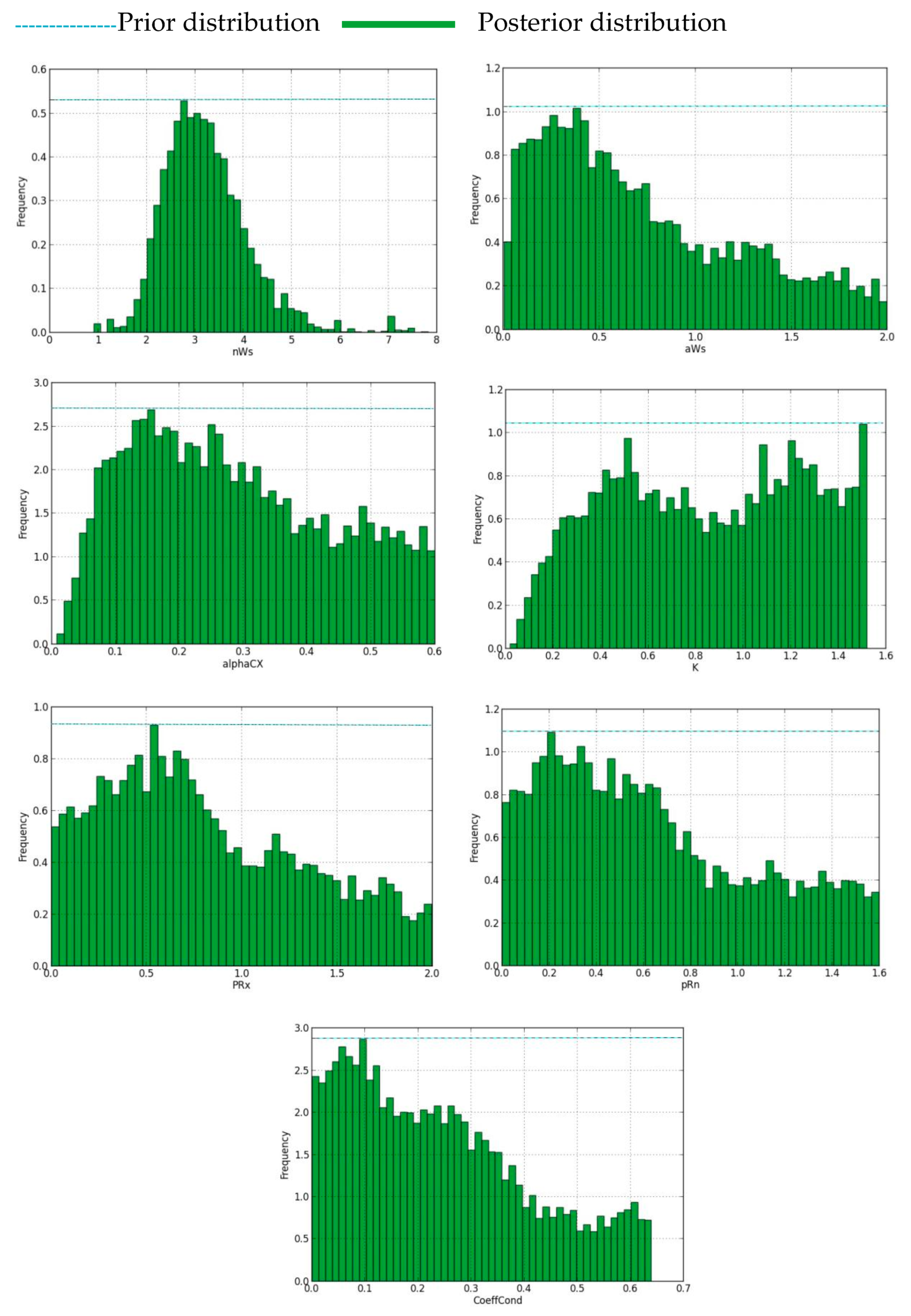
- The posterior probability distributions of nWs, aWs, alphaCx, pRx, pRn, and MaxCond have an approximately normal or skewed distribution with a prominent peak value; however, the peak value of k is not prominent, showing an irregular distribution.
- (4)
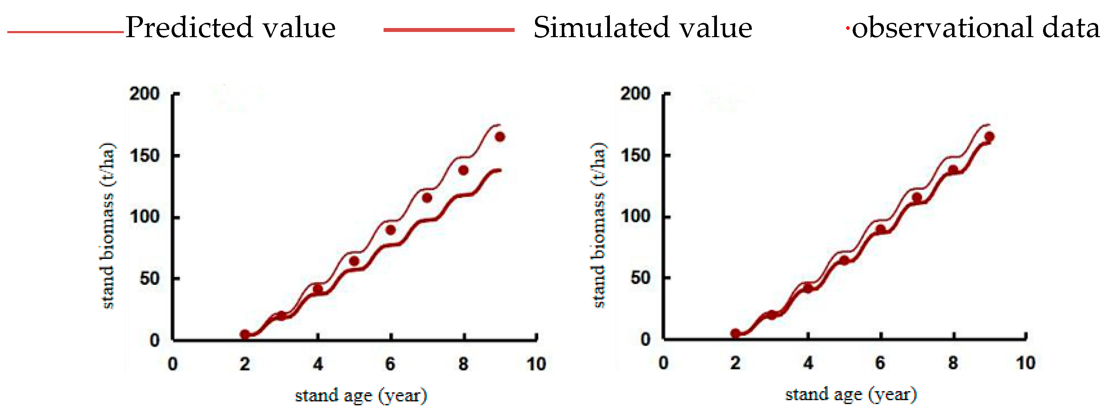
- Compared with the simulation results using the default parameters, the RMSEs of the stem values with the initial value (default parameter) and posterior value in the model simulation are 1.24 and 0.98, respectively; the RMSEs of the height values are 0.34 and 0.32, respectively; and the RMSEs of the DBH values are 0.71 and 0.69, respectively.
Author Contributions
Funding
Acknowledgments
Conflicts of Interest
References
- Luo, Y.; White, L.W.; Canadell, J.G.; DeLucia, E.H.; Ellsworth, D.S.; Finzi, A.; Lichter, J.; Schlesinger, W.H. Sustainability of terrestrial carbon sequestration: A case study in Duke Forest with inversion approach. Glob. Biogeochem. Cycles 2003, 17. [Google Scholar] [CrossRef]
- Raupach, M.R.; Rayner, P.J.; Barrett, D.J.; DeFries, R.S.; Heimann, M.; Ojima, D.S.; Quegan, S.; Schmullius, C.C. Model-data synthesis in terrestrial carbon observation: Methods, data requirements and data uncertainty specifications. Glob. Chang. Biol. 2005, 11, 378–397. [Google Scholar]
- Damian, J.B. Steady state turnover time of carbon in the Australian terrestrial biosphere. Glob. Biogeochem. Cycles 2002, 16, 55. [Google Scholar]
- Wang, Y.P.; Barrett, D.J. Estimating regional terrestrial carbon fluxes for the Australian continent using a multiple- constraint approach II. The Atmospheric constraint. Tellus B Chem. Phys. Meteorol. 2003, 55, 270–289. [Google Scholar]
- Rayner, P.J.; Scholze, M.; Knorr, W.; Kaminski, T.; Giering, R.; Widmann, H. Two decades of terrestrial carbon fluxes from a carbon cycle data assimilation system (CCDAS). Glob. Biogeochem. Cycles 2005, 19, GB2026. [Google Scholar] [CrossRef] [Green Version]
- Williams, M.; Schwarz, P.A.; Law, B.E.; Irvine, J.; Kurpius, M.R. An improved analysis of forest carbon dynamics using data assimilation. Glob. Chang. Biol. 2005, 11, 89–105. [Google Scholar]
- Luo, Y.; Weng, E.; Wu, X.; Gao, C.; Zhou, X.; Zhang, L. Parameter identifiability, constraint, and equifinality in data assimilation with ecosystem models. Ecol. Appl. 2009, 19, 571–574. [Google Scholar]
- Lin, J.C.; Pejam, M.R.; Chan, E.; Wofsy, S.C.; Gottlieb, E.W.; Margolis, H.A.; McCaughey, J.H. Attributing uncertainties in simulated biospheric carbon fluxes to different error sources. Glob. Biogeochem. Cycles 2011, 25. [Google Scholar] [CrossRef]
- Almeida, A.C.; Landsberg, J.J.; Sands, P.J. Parameterisation of 3-PG model for fast-growing Eucalyptus grandis plantations. For. Ecol. Manag. 2004, 193, 179–195. [Google Scholar]
- Metropolis, N.; Rosenbluth, A.W.; Rosenbluth, M.N.; Teller, A.H.; Teller, E. Equation of state calculations by fast computing machines. J. Chem. Phys. 1953, 21, 1087–1092. [Google Scholar] [CrossRef] [Green Version]
- Chib, S.; Greenberg, E. Understanding the Metropolis-Hastings algorithm. Am. Stat. 1995, 49, 327–335. [Google Scholar]
- Hastings W, K. Monte Carlo sampling methods using Markov chain and their applications. Biometrika 1970, 57, 97–109. [Google Scholar]
- Geman, S.; Geman, D. Stochastic Relaxation, Gibbs Distributions, and the Bayesian Restoration of Images. IEEE T. Pattern. Anal. 1987, 6, 721–741. [Google Scholar]
- Zobitz, J.M.; Desai, A.R.; Moore, D.J.P.; Chadwick, M.A. A primer for data assimilation with ecological models using Markov Chain Monte Carlo (MCMC). Oecologia 2011, 167, 599–611. [Google Scholar] [PubMed]
- Ren, X.; Honglin, H.; Moore, D.J.P.; Zhang, L.; Liu, M.; Li, F.; Yu, G.; Wang, H. Uncertainty analysis of modeled carbon and water fluxes in a subtropical coniferous plantation. J. Geophys. Res. Biogeosci. 2013, 118, 1674–1688. [Google Scholar]
- Ricciuto, D.M.; King, A.W.; Dragoni, D.; Post, W.M. Parameter and prediction uncertainty in an optimized terrestrial carbon cycle model: Effects of constraining variables and data record length. J. Geophys. Res. 2011, 116. [Google Scholar] [CrossRef] [Green Version]
- Landsberg, J.-J.; Waring, R.-H. A generalised model of forest productivity using simplified concepts of radiation-use efficiency, carbon balance and partitioning. For. Ecol. Manag. 1997, 95, 209–228. [Google Scholar]
- Hutchinson, M.F. The application of thin plate smoothing splines to continent-wide data assimilation. Data Assim. Syst. 1991, 27, 104–113. [Google Scholar]
- Coops, N.-C.; Waring, R.-H. Assessing forest growth across southwestern Oregon under a range of current and future global change scenarios using a process model, 3-PG. Glob. Chang. Biol. 2001, 7, 15–29. [Google Scholar]
- Esprey, L.-J.; Sands, P.-J.; Smith, C.-W. Understanding 3-PG using a sensitivity analysis. For. Ecol. Manag. 2004, 193, 235–250. [Google Scholar]
- Battaglia, M.; Sands, P. Application of sensitivity analysis to a model of Eucalyptus globulus plantation productivity. Ecol. Model. 1998, 111, 237–259. [Google Scholar] [CrossRef]
- Battagalia, M.; Sands, P.J. Process-based forest productivity models and their application in forest management. For. Ecol. Manag. 1998, 102, 13–32. [Google Scholar] [CrossRef]
- Song, X.; Bryan, B.A.; Almeida, A.C.; Paul, K.I.; Zhao, G.; Ren, Y. Time-dependent sensitivity of a process-based ecological model. Ecol. Model. 2013, 265, 114–123. [Google Scholar] [CrossRef]
- Song, X.; Bryan, B.A.; Paul, K.I.; Zhao, G. Variance-based sensitivity analysis of a forest growth model. Ecol. Model. 2012, 247, 135–143. [Google Scholar] [CrossRef]
- Mertens, J.; Madsen, H.; Feyen, L.; Jacques, D.; Feyen, J. Including prior information in the estimation of effective soil parameters in unsaturated zone modelling. J. Hydrol. 2004, 294, 251–269. [Google Scholar] [CrossRef]
- Seidel, S.J.; Palosuo, T.; Thorburn, P.; Wallach, D. Towards improved calibration of crop models: Where are we now and where should we go. Eur. J. Agron. 2018, 94, 25–35. [Google Scholar] [CrossRef]
- Gauch, H.G.; Hwang, J.G.; Fick, G.W. Model evaluation by comparison of model-based predictions and measured values. Agron. J. 2003, 95, 1442–1446. [Google Scholar] [CrossRef] [Green Version]
- Irmak, A.; Jones, J.W.; Batchelor, W.D.; Paz, J.O. Estimating spatially variable soil properties for application of crop models in precision. Agriculture 2001, 44, 1343. [Google Scholar] [CrossRef]
- Romanowicz, R.J.; Beven, K.J. Comments on generalised likelihood uncertainty estimation. Reliab. Eng. Syst. Saf. 2006, 91, 1315–1321. [Google Scholar] [CrossRef]
- Moulin, S.; Bondeau, A.; Delecolle, R. Combining agricultural crop models and satellite observations: From field to regional scales. Int. J. Remote Sens. 1998, 19, 1021–1036. [Google Scholar] [CrossRef]
- Iizumi, T.; Yokozawa, M.; Nishimori, M. Parameter estimation and uncertainty analysis of a large-scale crop model for paddy rice: Application of a Bayesian approach. Agric. For. Meteorol. 2009, 149, 333–348. [Google Scholar] [CrossRef]
- Marin, F.; Jones, J.W.; Boote, K.J. A stochastic method for crop models: Including uncertainty in a sugarcane model. Agron. J. 2017, 109, 483–495. [Google Scholar] [CrossRef]
- Kalnay, E.; Kanamitsu, M.; Kistler, R.; Collins, W.; Deaven, D.; Gandin, L.; Iredell, M.; Saha, S.; White, G.; Woollen, J.; et al. The NCEP/NCAR 40-year reanalysis project Bull. Am. Meteor. Soc 1996, 77, 437–471. [Google Scholar] [CrossRef] [Green Version]


| Month | Maximum Temperature/°C | Minimum Temperature/°C | Precipitation/mm | Solar Radiation (MJ*m2*d−1) | Frost Days/d |
|---|---|---|---|---|---|
| January | 22.45 | –1.88 | 36.29 | 25.45 | 0 |
| February | 23.94 | 2.16 | 89.38 | 23.27 | 0 |
| March | 24.53 | 4.02 | 915.97 | 19.85 | 0 |
| April | 25.51 | 10.69 | 146.07 | 14.36 | 0 |
| May | 26.96 | 13.95 | 148.8 | 10.08 | 0.67 |
| June | 27.6 | 18.39 | 224.55 | 7.91 | 2.25 |
| July | 28.58 | 21.43 | 187.58 | 8.46 | 3.75 |
| August | 27.97 | 21.99 | 295.55 | 11.82 | 2.5 |
| September | 27.18 | 17.36 | 210.4 | 15.62 | 0.33 |
| October | 25.9 | 9.75 | 33.53 | 20.44 | 0 |
| November | 23.79 | 3.83 | 21.32 | 23.61 | 0 |
| December | 21.43 | –0.44 | 35.42 | 25.64 | 0 |
| Parameter Name | Definition | Unit | Symbol | Value |
|---|---|---|---|---|
| pFS2 | Ratio of foliage:stem partitioning at B = 2 cm | - | p2 | 1 |
| pFS20 | Ratio of foliage:stem partitioning at B = 20 cm | - | p20 | 0.15 |
| aWS | Constant in stem mass vs. diameter relationship | - | aS | 0.095 |
| nWS | Power in stem mass vs. diameter relationship | - | nS | 2.4 |
| pRx | Maximum fraction of NPP to roots | - | ηRx | 0.8 |
| pRn | Minimum fraction of NPP to roots | - | ηRn | 0.25 |
| gammaF0 | Litterfall rate at t = 0 | month−1 | γF0 | 0.027 |
| gammaF1 | Litterfall rate for mature stands | month−1 | γF1 | 0.001 |
| tgammaF | Age at which litterfall rate has median value | month−1 | Ft | 12 |
| Rttover | Average monthly root turnover rate | month−1 | γR | 0.015 |
| Tmin | Minimum temperature for growth | °C | Tmin | 8.5 |
| Topt | Optimum temperature for growth | °C | Topt | 16 |
| Tmax | Maximum temperature for growth | °C | Tmax | 40 |
| kF | Number of production days lost for each frost day | days | kF | 0 |
| m0 | Value of m when FR = 0 | - | m0 | 0 |
| fN0 | Value of fN when FR = 0 | - | fN0 | 1 |
| fNn | Power of (1–FR) in fN | - | nfN | 0 |
| CoeffCond | Defines stomatal response to VPD | mbar | kD | 0.05 |
| fCalpha700 | Quantum efficiency at 700 ppm | - | fC700 | 0.7 |
| fCg700 | Canopy conductivity at 700 ppm | - | fCg700 | 0.7 |
| SWconst | Moisture ratio deficit which gives fθ= 0.5 | - | c | 0.7 |
| SWpower | Power of moisture ratio deficit in fθ | - | n | 9 |
| MaxAge | Maximum stand age used to compute relative age | yr | tx | 50 |
| nAge | Power of relative age in fage | - | nage | 4 |
| rAge | Relative age to give fage = 0.5 | - | rage | 0.95 |
| MinCond | Minimum canopy conductance | m s−1 | gCn | 0 |
| MaxCond | Maximum canopy conductance | m s−1 | gCx | 0.02 |
| LAIgcx | Canopy LAI for maximum canopy conductance | m2 m−2 | LCx | 3.33 |
| BLcond | Canopy boundary layer conductance | m s−1 | gB | 0.2 |
| gammaN0 | Seedling mortality rate (t = 0) | yr−1 | N0 | 0.03 |
| gammaNx | Mortality rate for older stands (large t) | yr−1 | N1 | 0.001 |
| tgammaN | Age at which γN = 1/2(γN0+γN1) | yr | tN | 12 |
| ngammaN | Shape of mortality response | - | nN | 0.015 |
| wSx1000 | Maximum stem mass per tree at 1000 trees/ha | kg/tree | wSx1000 | 300 |
| thinPower | Power in self-thinning law | - | nN | 3/2 |
| mF | Fractions of mean foliage, root, and stem biomass pools per tree on each dying tree | - | mF | 0 |
| mR | - | mR | 0.2 | |
| mS | - | mS | 0.2 | |
| SLA0 | Specific leaf area at a stand age of 0 | m2 kg−1 | σ0 | 11 |
| SLA1 | Specific leaf area for mature stands | m2 kg−1 | σ1 | 4 |
| tSLA | Age at which specific leaf area = (SLA0+SLA1)/2 | yr | t | 2.5 |
| MaxIntcptn | Maximum fraction of rainfall intercepted by canopy | - | iRx | 0.15 |
| LAImax-Intcptn | LAI for maximum rainfall interception | m2 m−2 | Lix | 0 |
| k | Extinction coefficient for PAR absorption by canopy | - | k | 0.5 |
| fullCanAge | Age at full canopy cover | yr | tc | 0 |
| alphaCx | Maximum canopy quantum efficiency | - | Cx | 0.06 |
| Y | Ratio NPP/GPP | - | Y | 0.47 |
| fracBB0 | Branch and bark fraction at a stand age of 0 | - | p | 0.75 |
| fracBB1 | Branch and bark fraction for mature stands | - | p | 0.15 |
| tBB | Age at which pBB = 1/2(PBB0+ PBB1) | yr | tBB | 2 |
| rhoMax | Minimum basic density for young trees | t m−3 | ρ0 | 0.5 |
| Maximum basic density for older trees | t m−3 | ρ1 | 0.5 | |
| tRho | Age at which p = 1/2 density of old and young trees | yr | tρ | 4 |
| aH | Constant in stem diameter to height relationship | yr | aH | 0 |
| nHB | Power of DBH in stem height relationship | - | nHB | 0 |
| nHN | Power of stocking in stem height relationship | - | nHN | 0 |
| aV | Constant in stem diameter to volume relationship | - | aV | 0 |
| nVB | Power of DBH in stem volume relationship | - | nVB | 0 |
| nVN | Power of stocking in stem volume relationship | - | nVN | 0 |
| Qa | Intercept in net radiation vs. solar radiation relationship | W m−2 | Qa | −90 |
| Qb | Slope of net radiation vs. solar radiation relationship | - | Qb | 0.8 |
| gDM_mol | Molecular weight of dry matter | g mol−1 | 24 | |
| molPAR_MJ | Conversion of solar radiation to PAR | mol MJ−1 | 2.3 |
| Parameter | Sensitivity Value (λ1) | Grade (λ1) | ||
|---|---|---|---|---|
| StemNo | DBH | StemNo | DBH | |
| nWS | –0.06 | –3.10 | 0 | 3 |
| aWS | –0.02 | –0.21 | 0 | 1 |
| alphaCx | 1.17 | 0.48 | 3 | 3 |
| k | 0.21 | 0.09 | 1 | 1 |
| pRx | –0.35 | –0.13 | 2 | 1 |
| pRn | –0.50 | –0.21 | 3 | 1 |
| CoeffCond | –0.73 | –0.31 | 3 | 2 |
| Parameter | Unit | Initial Value | Range | Mode | Mean + SD |
|---|---|---|---|---|---|
| nWS | - | 2.4 | [0,8] | 2.76 | 3.08 ± 0.17 |
| aWS | - | 0.095 | [0,2] | 0.42 | 0.58 ± 0.02 |
| alphaCx | - | 0.06 | [0,0.6] | 0.16 | 0.26 ± 0.1 |
| k | - | 0.5 | [0,1.5] | 1.04 | 0.80 ± 0.24 |
| pRx | - | 0.6 | [0,2] | 0.56 | 0.71 ± 0.09 |
| pRn | - | 0.25 | [0,1.6] | 0.24 | 0.59 ± 0.1 |
| CoeffCond | 1/mbar | 0.05 | [0,0.65] | 0.11 | 0.24 ± 0.01 |
| Height | DBH | Stand Biomass | ||||
|---|---|---|---|---|---|---|
| Before Optimization | After Optimization | Before Optimization | After Optimization | Before Optimization | After Optimization | |
| RMSE | 0.34 | 0.32 | 0.71 | 0.69 | 1.24 | 0.98 |
Publisher’s Note: MDPI stays neutral with regard to jurisdictional claims in published maps and institutional affiliations. |
© 2020 by the authors. Licensee MDPI, Basel, Switzerland. This article is an open access article distributed under the terms and conditions of the Creative Commons Attribution (CC BY) license (http://creativecommons.org/licenses/by/4.0/).
Share and Cite
Liu, C.; Zheng, X.; Ren, Y. Parameter Optimization of the 3PG Model Based on Sensitivity Analysis and a Bayesian Method. Forests 2020, 11, 1369. https://doi.org/10.3390/f11121369
Liu C, Zheng X, Ren Y. Parameter Optimization of the 3PG Model Based on Sensitivity Analysis and a Bayesian Method. Forests. 2020; 11(12):1369. https://doi.org/10.3390/f11121369
Chicago/Turabian StyleLiu, Chenjian, Xiaoman Zheng, and Yin Ren. 2020. "Parameter Optimization of the 3PG Model Based on Sensitivity Analysis and a Bayesian Method" Forests 11, no. 12: 1369. https://doi.org/10.3390/f11121369