A New Method for Forest Canopy Hemispherical Photography Segmentation Based on Deep Learning

Abstract

Research Highlights: This paper proposes a new method for hemispherical forest canopy image segmentation. The method is based on a deep learning methodology and provides a robust and fully automatic technique for the segmentation of forest canopy hemispherical photography (CHP) and gap fraction (GF) calculation. Background and Objectives: CHP is widely used to estimate structural forest variables. The GF is the most important parameter for calculating the leaf area index (LAI), and its calculation requires the binary segmentation result of the CHP. Materials and Methods: Our method consists of three modules, namely, northing correction, valid region extraction, and hemispherical image segmentation. In these steps, a core procedure is hemispherical canopy image segmentation based on the U-Net convolutional neural network. Our method is compared with traditional threshold methods (e.g., the Otsu and Ridler methods), a fuzzy clustering method (FCM), commercial professional software (WinSCANOPY), and the Habitat-Net network method. Results: The experimental results show that the method presented here achieves a Dice similarity coefficient (DSC) of 89.20% and an accuracy of 98.73%. Conclusions: The method presented here outperforms the Habitat-Net and WinSCANOPY methods, along with the FCM, and it is significantly better than the Otsu and Ridler threshold methods. The method takes the original canopy hemisphere image first and then automatically executes the three modules in sequence, and finally outputs the binary segmentation map. The method presented here is a pipelined, end-to-end method.

1. Introduction

1.1. Background

The forest canopy is the interface that directly interacts with the external atmospheric environment in the forest ecosystem. It integrates the most active biological components in the forest ecosystem [1]. The forest canopy structure not only determines the energy exchange of water, heat, air, light, and other substances between the arboreal layer and the external environment, but also affects many physiological and environmental factors such as understory vegetation and the soil environment, ultimately affecting the growth trend for the whole forest community [2]. Therefore, the acquisition of forest canopy structure parameters is very important for forest growth monitoring, biomass estimation, and forest growth simulation models.

Canopy hemispherical photography (CHP) technology can easily, quickly, and non-destructively measure the structural parameters of a forest canopy, such as the gap fraction (GF), clumping index, and leaf area index (LAI), etc. The GF is one of the most important forest canopy parameters. A change in canopy GF reflects a change in canopy structure and canopy growth, and provides an important theoretical basis for studying canopy characteristics and changes. In addition, the LAI, average leaf inclination angle, and clumping index can all be obtained by deduction from the GF. The calculation of the GF often includes the segmentation of hemispherical images as a prerequisite.

1.2. Related Works

Gap fractions have often been used to estimate the foliage densities of canopies based on different canopy models, thereby estimating LAI values. Research on CHP image segmentation methods has been active since the 1980s. Threshold methods select a gray value to separate the sky and vegetation pixels in the images, which is referred to as binary segmentation. Lee [3] used variable threshold technology (including optimal color channel selection and optimal threshold determination) to monitor the changes in the foliage area of a Douglas fir canopy infested by tussock moths, providing a quantitative method for the growth loss assessment of insect-infested trees. Leblanc [4] extracted the structural parameters (i.e., GF, clustering index, and plant area index (PAI)) of a boreal forest canopy. Each image was segmented independently using the dual threshold method in order to minimize multiple scattering differences in the canopy, the difference in sky radiance, and any vignetting effect of the lens; however, the threshold needs to be manually assigned, which is not an automatic process.

Another automatic threshold method is based on image histogram analysis. Ishida [5] used the maximum curvature point of the L-shaped curve in a hemispheric image histogram as the threshold, where the correlation between “DIFphoto” (i.e., diffuse transmittance as calculated by the CHP) and “DIFsensor” (i.e., diffuse transmittance as measured with a photosynthetic photon flux density sensor) reached 0.99. They found that digital hemispherical photography with automatic exposure control overestimated open sky and diffuse transmittance under dense canopies. Juárez [6] used the minimum histogram entropy difference to determine the optimal threshold to distinguish between the sky and foliage of an Amazonian forest canopy. According to the segmentation results, the GF of the canopy can be calculated and accurate estimates of the LAI can be obtained. Macfarlane [7] proposed a dual-angle method (dual threshold) based on an image histogram. The method systematically quantifies the number of mixed pixels in canopy images and demonstrates that fisheye images contain more mixed pixels than cover images, and that the number of mixed pixels increases with increasing vegetation cover.

Other studies have only comparatively studied the existing methods, such as those of Mizoue [8], Jonckheere [9], Inoue [10], and Glatthorn [11] et al. In these studies, for hemispherical images with different weather conditions and different canopy densities, the performances of various segmentation algorithms were different, but the differences were not significant. Woodgate [12] compared three common classification algorithms for CHP segmentation, namely manual supervision classification, a global binary threshold method, and dual-angle automatic threshold methods. They concluded that the estimated error of the supervised classification method and the dual-angle method for the GF and LAI was less than 10%. The global threshold method overestimates the canopy opening and GF, but underestimates the LAI.

Other methods are based on edge detection (e.g., the Nobis method [13]), and clustering technology (e.g., the Pueschel method [14]); however, for the latter, the number of clusters needs to be assigned and assumes that the sky brightness is uniform.

A CHP image segmentation algorithm based on machine learning uses image features to train a classifier and then uses the trained classifier to classify all the pixels in the image to complete the segmentation tasks, which has gradually become a research focus in recent years. Diaz [15] used object-based image analysis (OBIA) to identify the canopy GF of a broadleaf stand of Nothofagus pumilio. Diaz pointed out that the color and texture features of hemispherical images can also be used to extract the GF, but automatic exposure will overestimate the GF. Huang et al. [16] proposed a rice canopy image segmentation method based on the color features and a support vector machine (SVM). The experimental data were captured under overcast, cloudy, and sunny sky conditions and achieved higher segmentation accuracy than other methods. Zhao et al. [17] compared the U-Net convolutional neural network (CNN) with a region-based CNN network (R-CNN) mask in terms of the performances of pomegranate tree canopy segmentation and found that the R-CNN mask achieved much better performance than the U-Net method. Wagner [18] used a U-Net CNN to segment remote sensing images (WorldView-3 images) of the Atlantic Forest to identify forest types. Abramsa [19] proposed a Habitat-Net network to segment canopy images in tropical rainforest habitats. The essence of the network is a U-Net CNN with batch normalization, which achieves high accuracy (DSC = 0.94); however, the image data are digital cover photographs (DCP) rather than CHP images. CHP image segmentation methods based on deep learning have rarely been reported in the literature. CHP images are acquired by photographing the forest canopy from down to up with a fisheye lens. The principle of hemispherical image projection is shown in Figure 1, where θ and φ are the azimuth angle and zenith angle of P on the spherical surface, respectively, and p is the corresponding pixel point in the hemispherical image plane. In addition to the distortion of the fisheye lens, the contrast in forest CHP is poor due to the direct sunlight, the cloud reflection, the leaf refraction, environmental scattering, and other ambient light factors, which makes the segmentation of CHP images more challenging than DCP images.

This paper proposes a fully automatic canopy image segmentation method based on deep learning, which consists of a preprocessing module and a segmentation module. It is an end-to-end method for canopy image segmentation. It can provide a standard processing flow for the calculation of a forest canopy GF and estimation of the LAI.

2. Materials and Methods

2.1. Method Overview

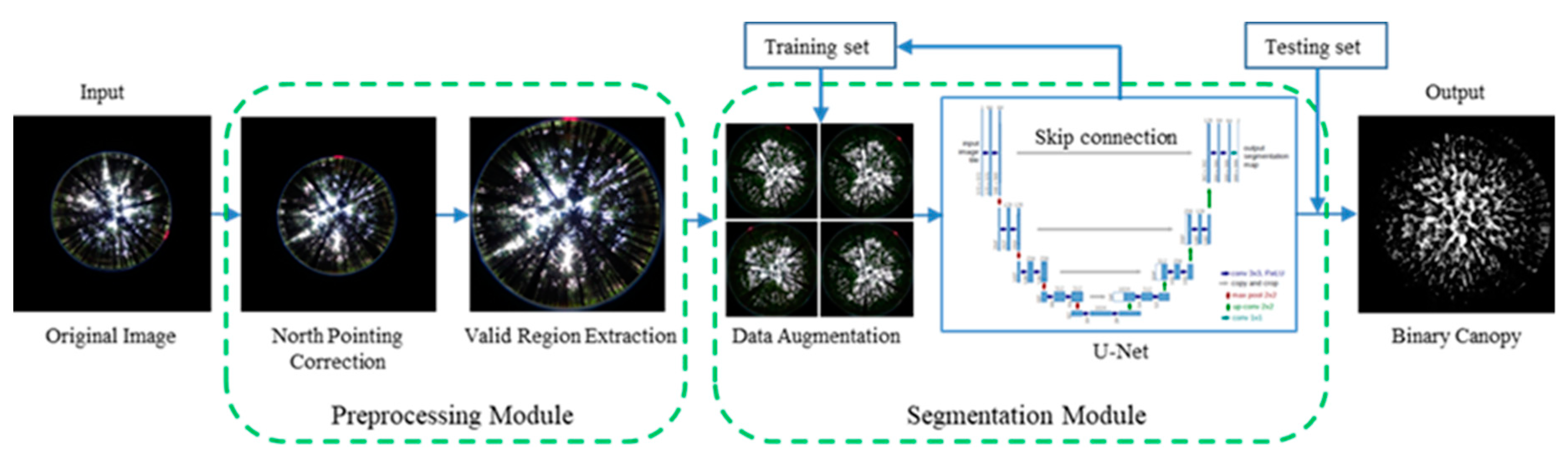
The overall process of the method is shown in Figure 2.

The method includes two parts, namely, an image preprocessing module and a canopy image segmentation module. The preprocessing module performs the two major tasks of northing correction and the circular valid region extraction, and the cropped image (the valid region image) is sent to the hemispherical image segmentation module. The image segmentation module is a deep segmentation model based on the U-Net network. The U-Net details are described in Figure 5. The training of this model requires a large quantity of data. Therefore, the image data need to be augmented. Then, the augmented canopy images are fed to the U-Net model for learning, and a deep segmentation model of the canopy hemisphere image is obtained. Finally, the test set is inserted into the segmentation model and the results of the binarized canopy images are produced as an output. The detailed steps of each module are described below.

2.2. Acquisition of CHP Data

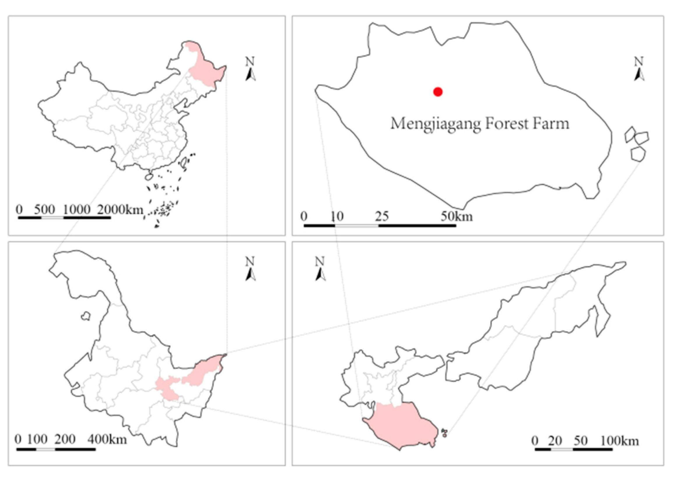
The CHP data (3135 images) were acquired at the Mengjiagang Forest Farm in Jiamusi, Heilongjiang Province, China. The geographical coordinates of the site are 130°32′42′′–130°52′36′′ E and 46°20′16′′–46°30′50′′ N. The site is shown in Figure 3. The data acquisition time was from 9 to 26 August 2017. The forest types there are Korean pine (Pinus koraiensis Sieb. et Zucc.), Scots pine (Pinus sylvestris L. var. mongholica Litv.), and Korean spruce (Picea koraiensis Nakai). The camera and lens were attached to a self-leveling mount, which was oriented by corner pins on a tripod. This configuration ensured a consistent level positioning for the camera during image acquisition. The top of the lens was located 1.3 m above the ground and the camera was oriented such that the magnetic north was always located at the top of the photographs. Photographs were taken from 10 a.m. to 3 p.m. under the conditions of diffused skylight (i.e., overcast), with automatic exposure settings. Images were captured using a DMC-LX5 camera (Matsushita Electric Industrial Co., Ltd., Osaka, Japan) with a fisheye lens at the highest resolution (2736 × 2736 pixels). After the valid region is extracted, the image resolution is changed to 1678 × 1678. By limitation of the memory in our workstation, the 1000 images with 1678 × 1678 are still out of memory when training the U-NET model. In order to make the script run successfully, we resized the images to 1024 × 1024.

2.3. CHP Image Preprocessing

The image preprocessing module includes two steps, namely, the northing correction algorithm and valid region extraction.

2.3.1. Northing Correction Algorithm

From an ecological standpoint, the northing correction of fisheye images helps to ensure the azimuth consistency of canopy hemisphere images taken at different times, and this makes it easy to compare dynamic ecological parameters such as the GF and LAI, which is of great significance.

The algorithm consists of three steps, namely, red spot detection, region centroid calculation, and rotation angle calculation. The implementation details are given in Algorithm 1.

Algorithm 1. Procedure for the Northing Correction.

Input: The valid region image f, the threshold T1, T2, and T3 of the red, green, and blue components (denoted as f1, f2, and f3).

Output: The image after correction

Begin

1. For each pixel, DO 2. If (f1(x, y) > T1 and f2(x, y) < T2 and  f3(x, y) < T3) = false, then f1(x, y) = f2(x, y) = f3(x, y) = 0; 3. Perform open operation on f(x, y), End 4. For each pixel, DO 5. If (f1 > T1 and f2 < T2 and f3 < T3), then count the horizontal and vertical coordinates and the total number of coordinates 6. Calculate the centroids Xc, Yc; End 7. Determine the triangle vertex; 8. Calculate the side length of triangle; 9. Calculate the cosine of the triangle; 10. Calculate the arc cosine; 11. Radian converted to angle value; 12. Rotate the image according to the angle.

End

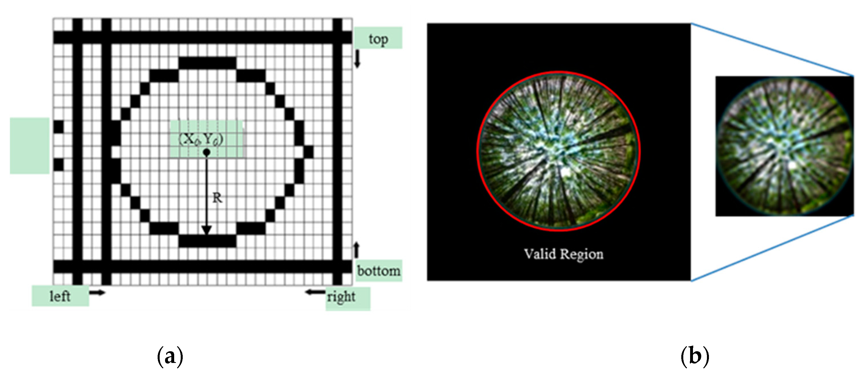
2.3.2. Valid Region Extraction

The forest CHP images captured by the fisheye lens have large low pixel value areas between the circular boundary and the image boundary. In order to reduce the memory usage and improve the data processing efficiency, the low pixel value region needs to be removed, and only the circular valid area containing the canopy is retained. Here, a scanning and cutting algorithm is used to extract valid regions [20]. The principle of the scanning algorithm and the schematic of the valid region are shown in Figure 4.

Since the CHP images are color images, they need to be converted to grayscale images before the scanning algorithm is used. The gray scale transformation formula is shown below.

L = 0.30R + 0.59G + 0.11B

(1)

where R, G, and B are the red, green, and blue components of the color canopy images, and L denotes the grayscale image converted from the color components.

The algorithm steps for the scanning method are shown in Algorithm 2.

Algorithm 2. Procedure for the Valid Region Extraction.

Input: A DHP I and a threshold T;

Output: The valid region image Ivr;

Begin

1. Convert I to a gray image L using Equation (1); 2. Determine the scanning direction (row Y or column X);

3. Start scan;

4. Compute intensity L of each pixel on the scan line;

5. Compute maximum intensity difference Llim on the scan line;

6. Compare Llim with T, if L lim > T in line 7, else return to line 3;

7. Stop scan;

8. Record the position of the scan line, denoted as X left, X right, Ytop, Ybottom;

9. Compute the center X0, Y0 and the radius R of the valid region;

10. Crop and output the Ivr.

End

The output of the scanning algorithm is the valid circular image, which is prepared as an input to the next segmentation module.

2.4. CHP Image Segmentation

Image segmentation technology based on deep learning has attracted great attention from researchers in recent years. It has first been applied to segmentation tasks for natural scene images (Refer to photos of daily life taken by people with mobile phones and digital cameras) or medical images, and then gradually extended to the research field of botany or ecology [21]; however, applications of deep learning techniques in these fields are immature. Botanists, ecologists, and computer vision experts need to transplant deep segmentation models into the ecology field and modify them to develop CHP image segmentation models. This paper develops a lightweight and efficient deep segmentation model that is suitable for use with hemispherical forest canopy images.

2.4.1. Data Preparation

(1)

Data augmentation

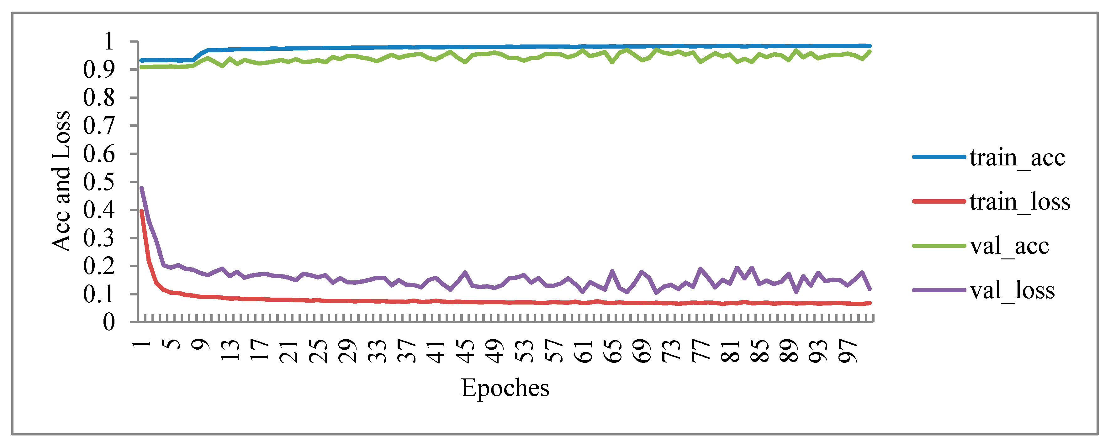
Deep learning typically requires a large quantity of data for training or else overfitting will occur, meaning that data augmentation is necessary. Generally speaking, our data sets are captured in limited scenes. However, our target application may exist in different conditions, such as in different directions, positions, zoom ratios, brightness, etc. We can use additional synthetic data to train a neural network to explain these situations. The data augmentation method used in this paper includes flipping, translation, rotation, and scaling. Augmentation was performed with the Keras deep learning API, and the number of augmented images was about 100,000 with a setting of 100 epochs (all samples in the data set are run once and called an epoch). The augmented images and the corresponding manual reference images pairs were fed to the U-net model for training.

(2)

Parameters setting

A total of 1295 CHP images were selected after removing some images with direct sunlight. In the experiments, the training/validation/test sets were divided into sets of 1000/195/100 randomly. The TensorFlow framework was used with a Linux system, and the Habitat-Net method and our method used the same parameter settings. The parameters that were used are given as follows: Learning rate set to 0.001, batch size set to 2, and number of epochs set to 100. We used Adam as the optimizer and the training time was about 8 h. The workstation was configured with 2 NVIDIA Titan XP GPUs and the available RAM size as 24 GB. The fuzzy clustering method (FCM) parameter settings are given as follows: The maximum number of iterations was 25, the cluster number was 2, and the minimum improvement was 0.001.

The FCM, Otsu, and Ridler algorithms were implemented using MATLAB R2017b with a PC configured with a 3.0 GHz CPU and a 4 GB of RAM. We used WinSCANOPY 2003 to perform image analysis.

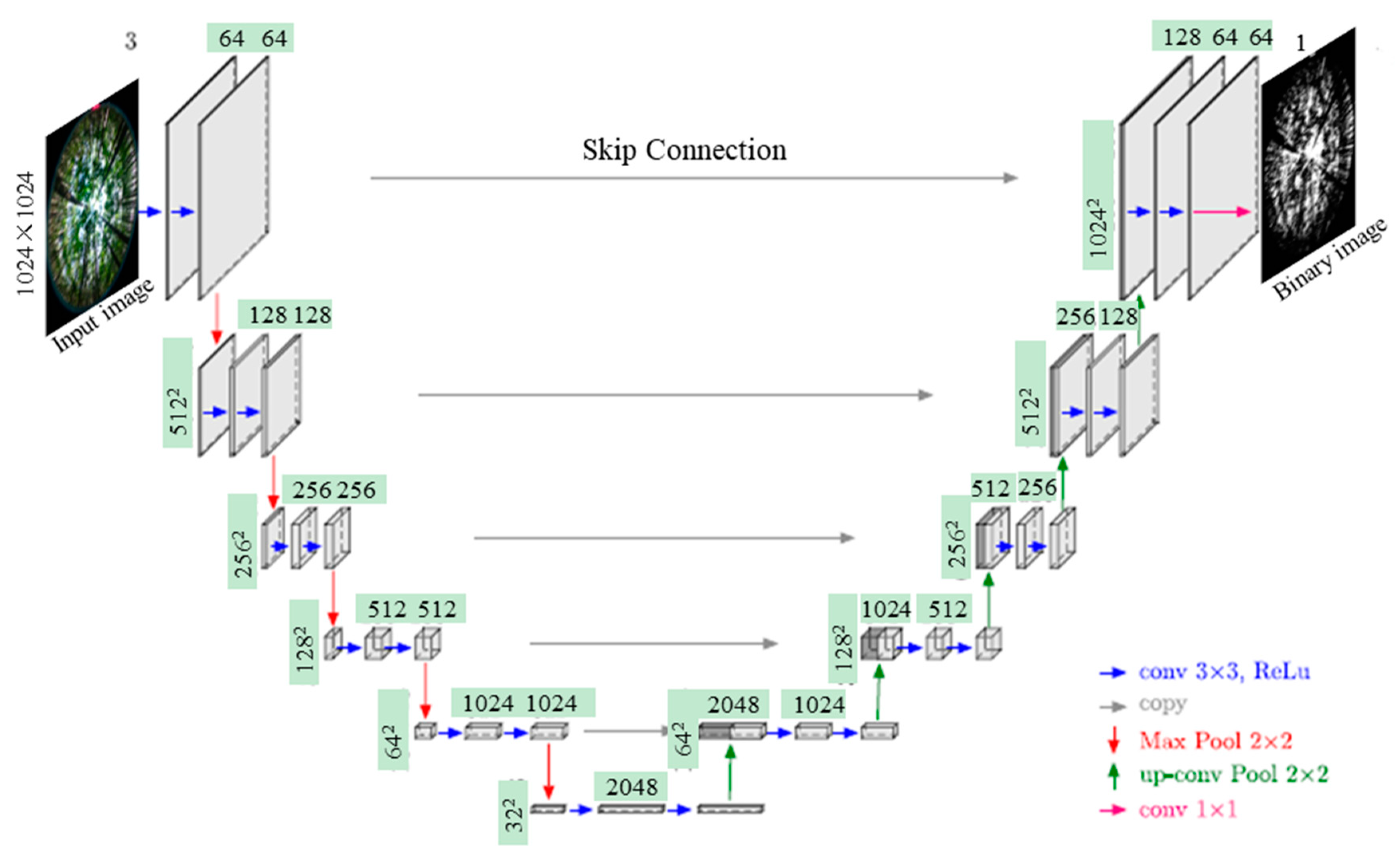
2.4.2. U-Net Architecture

Compared with other convolutional neural networks, the U-Net network extracts features of the canopy image and transfers the location information of the features to the corresponding layer through a skip connection as to keep the location information of features in the image as much as possible. This has unique significance for the accurate segmentation of forest canopies and GF calculation. The U-Net network used in this paper was composed of 23 convolutional layers, 5 pooling layers, and 5 upsampling layers, as shown in Figure 5. The most primitive U-Net model was first proposed by Ronneberger et al. in 2015, and was applied to the segmentation of biomedical images. The model is referred to as “U-Net” because its architecture is similar to a U-shaped distribution. It is a lightweight deep convolutional neural network (CNN) segmentation model.

The U-Net model consists of two parts, namely, a contraction path (left) and an expansion path (right). The network does not have a fully connected layer, where only a convolutional layer is used, and each convolutional layer is followed by a rectified linear units (Relu) activation function layer and then a pooling layer. The U-Net architecture is symmetrical and a skip connection is used. The skip connection helps restore the information loss caused by downsampling and can preserve finer image features. The network structure is also an encoder–decoder structure.

After the input images are downsampled 5 times and upsampled 5 times, the high-level semantic feature map obtained by the encoder is restored to the resolution of the original image, and the final image segmentation result is obtained.

2.5. Other Segmentation Methods

The Otsu traditional threshold method is a global automatic threshold segmentation method based on the maximum interclass variance, and the Ridler method is a segmentation algorithm that iteratively seeks the optimal threshold. FCM is an unsupervised machine learning method which uses a membership function to group canopy images into two categories, namely, sky and non-sky. WinSCANOPY also uses an automatic threshold method to segment hemispherical images. It calculates the proportion of the sky that can be observed upward from the bottom of the forest canopy. A value of 0 means that the sky cannot be seen at all (full covered), a value of 1 means the full sky, and values of 0–1 means that part of the sky is covered by leaves. The software uses the inverse program of the gap fraction to split the canopy image into several sectors or grids according to the partition number of the zenith angle and azimuth angle defined by the user, and automatically and quickly counts the pixels of the visible sky in each sector. Thus, the visible sky ratio (direct sunlight transmission coefficient) of the sector can be analyzed. The Habitat-Net and U-Net methods are both supervised machine learning and deep learning methods. Habitat-Net modified the original network structure and reduced the number of U-Net channels by a factor of two, making it more suitable for small-size image segmentation; however, the resolution of the CHP images is high (2736 × 2736), and a deeper and wider network architecture is consequently required.

2.6. Metrics of Segmentation Performance Evaluation

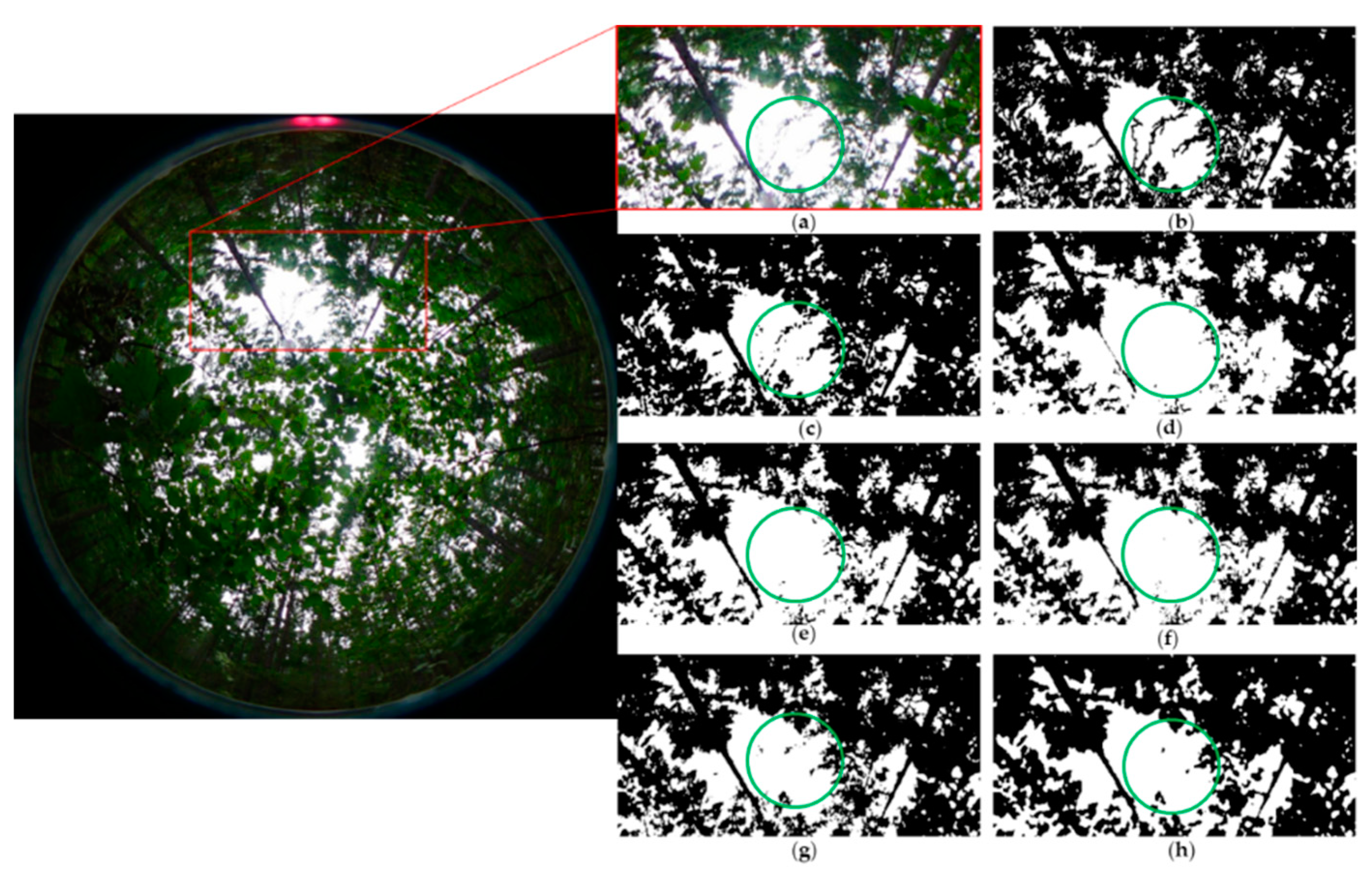
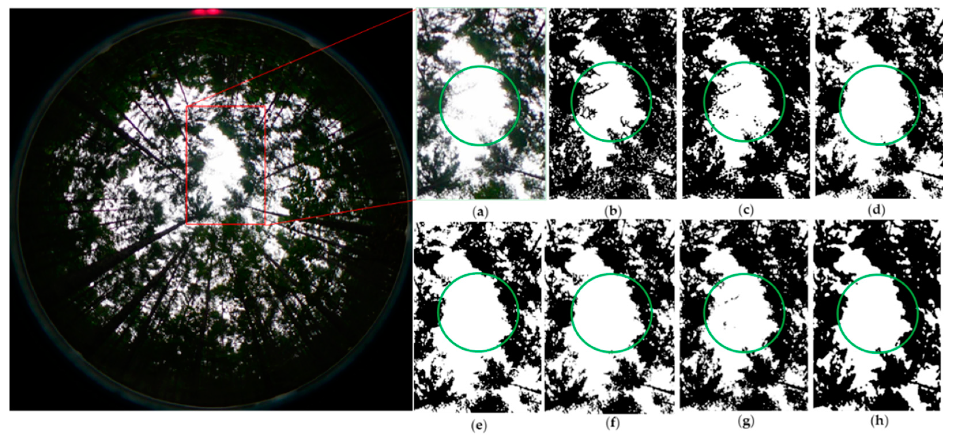
The manual reference images of the preprocessed canopy images were produced manually. We first used a simple threshold method to perform coarse segmentation for the canopy images and then used the overlay function of the ImageJ software package to manually revise the details for the canopy image. For example, we manually darkened the reflective regions of tree trunks, finely tuned the mixing area of the foliage and the sky, and bridged thin branches broken by strong light. This process is very time consuming. Under the supervision of the ecologist professor Zhihu Sun, it took 4 students 4 weeks to find the manual reference images for all of the images used here.

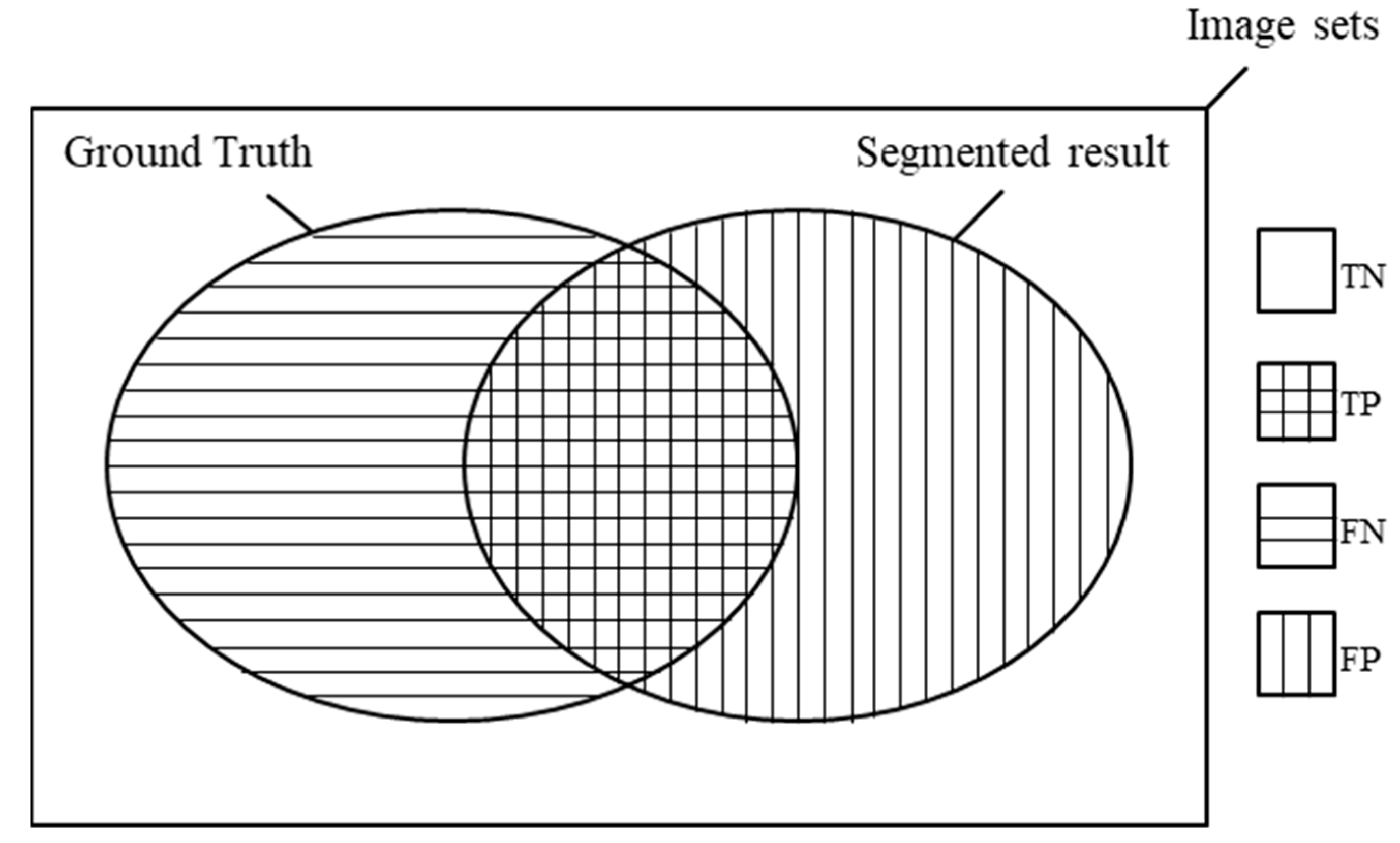
This paper uses the Dice similarity coefficient (DSC) and accuracy to evaluate the segmentation results. The DSC is a measure of the similarity between two sets. It is used in the field of image segmentation to measure the similarity between the network segmentation result and the gold standard mask. The DSC is defined as follows [22]:

$$\begin{gathered} \mathrm{DICE}=\frac{2·\left(V_{pred}{{\displaystyle \cap }}^{}{V}_{gt}\right)}{V_{pred}{{\displaystyle \cup }}^{}{V}_{gt}} \\ =2·\mathrm{TP}/\left(2·\mathrm{TP}+\mathrm{FP}+\mathrm{FN}\right) \end{gathered}$$

(2)

where $V_{gt}$ represents the manual reference images and $V_{pred}$ represents the segmented results. The numerator of the Equation (2) represents the intersection of two sets, and represents the correct area predicted by the algorithm, denoted by TP. When the prediction is completely correct, the two regions will overlap, and Dice is equal to 1. Its value is from 0 to 1.

The accuracy index is defined as follows, and it is performed at the pixel level [23]:

$$\mathrm{Accuracy}=\left(\mathrm{TP}+\mathrm{TN}\right)/\left(\mathrm{TP}+\mathrm{TN}+\mathrm{FP}+\mathrm{FN}\right)$$

(3)

where TP is true positive and denotes that the predicted result is sky and the manual reference images is sky; FP is false positive, denoting that the predicted result is sky and the manual reference images are foliage; TN is true negative, denoting that the predicted result is foliage and the manual reference images are foliage; and FN is false negative, denoting that the predicted result is foliage and the manual reference images are sky. It is illustrated in Figure 6.

The DSC refers to the proportion of black pixels, such as branches and canopy, that are correctly predicted to the entire set of image pixels. Accuracy refers to the ratio of the predicted correct black pixels, such as branch and canopy pixels, and the white pixels of the sky to the sum of the pixels of the two images, i.e., the manual reference images and the segmented images.

3. Experimental Results

3.1. Results of Segmentation for CHP

The segmentation results for four CHP images using different methods are shown in Figure 7. These segmentation methods were a threshold method, clustering method, the WinSCANOPY method, the Habitat-Net method, and our method based on U-Net.

It can be seen from Figure 7 that the traditional threshold segmentation methods such as the Otsu and Ridler methods obviously overestimate the GF of the canopy. This can be explained in Figure 8. The top row is the overlay of segmented images and manual reference images, while the bottom is the details for local enlargement. We use red to represent manual reference images, and green represents segmentation results. It can be seen from Figure 8b,d that the green areas are an overestimated sky, thus overestimating the GF. However, it can be seen from (f) that the green region has some scattered points, and the overestimated sky can be ignored. The comparisons are made under the same region in the three figures. The segmentation results for the WinSCANOPY and deep learning-based models (Habitat-Net and U-Net) are better and approximate the manual reference images; however, human–computer interaction is needed to complete the canopy image segmentation with the WinSCANOPY professional software, which is not a fully automatic process. Our method and the Habitat-Net method are end-to-end image segmentation methods. The algorithms take the original images and output segmented binary images. The whole process does not require manual intervention; however, both the segmentation precision and accuracy of our method are optimal, and it only takes about 450 ms to segment an image (1024 × 1024).

In order to further illustrate the segmentation advantages of our method, the segmentation details of the local area for a Korean pine broad-leaved mixed forest are shown in Figure 9.

It can be seen from Figure 9 that the brightness of the sky in the green box is saturated due to underexposure, and the small foliage in the box is significantly affected by the heavy sunlight. Traditional threshold segmentation methods (Otsu and Ridler) and clustering methods can hardly distinguish small foliage from a heavy sunlight background, while the U-Net network can segment as much small foliage as possible under the same environment.

Figure 10 is a segmentation display of the local area of the CHP images for a Korean pine forest. It is difficult to distinguish small foliage from the heavy sunlight background. It is shown in this scene that the sky and the foliage cannot be clearly discriminated with a separation task for the mixed pixels. Our U-Net network shows the best performance when it deals with this scene, and can extract more details than the other methods, such as the clustering method, WinSCANOPY, and Habitat-Net method. The traditional threshold methods (Otsu and Ridler methods) obviously failed for this mixed pixel classification scene.

The loss and accuracy curves of the image segmentation model during the training process are shown in Figure 11.

It can be seen from Figure 11 that the accuracy of the training set (blue line) was basically stable after 10 epochs. The loss curve (red line) was still decreasing, but the drop was small. It can be seen that the convergence of the model is fast; however, for the accuracy and loss curves of the validation set, there are some slight oscillations. The reason for this may be because the batch size or the learning rate is too small, or it may be the result of the joint action of the two parameters.

3.2. Comparison of Algorithms

In order to verify the segmentation performance of our method, we made a comparative study with automatic threshold methods (i.e., the Otsu and Ridler methods), a clustering method, the WinSCANOPY commercial software, and the Habitat-Net method. The test set consisted of 100 CHP images. DSC and accuracy were used to evaluate the segmentation performance of our model. The larger the DSC, the better the segmentation results reflect the manual reference images. We used the manual segmentation of the images as the manual reference images. The algorithm comparison results are shown in

Table 1. Results for the six segmentation methods. DSC: Dice similarity coefficient.

Metrics	Otsu	Ridler	FCM	WinSCANOPY	Habitat-Net	U-Net
DSC	62.89 ± 0.038%	62.14 ± 0.033%	63.49 ± 0.036%	74.19 ± 0.039%	77.59 ± 0.029%	89.20 ± 0.028%
Accuracy	92.54 ± 0.012%	92.32 ± 0.010	92.74 ± 0.010%	95.71 ± 0.008%	96.53 ± 0.006%	98.73 ± 0.004%

. The values in the table are the means and standard deviations of the DSC and accuracy for all test sets (100 images).

4. Discussion

When traditional threshold segmentation methods (Otsu and Ridler methods) are applied to canopy images they require neither a training model nor manual reference images, which saves a lot of time; however, the segmentation accuracies of these methods are not high, and their robustness is poor. The segmentation results are good for some images, but they will be poor when the image quality has deteriorated. The FCM algorithm uses the degree of membership to determine the degree of clustering for each data point, which is an improvement over the traditional hard clustering algorithm. It is sensitive to the initial clustering center and needs to manually determine the number of clusters, which makes it easy to fall into a local optimal solution. The presented method based on deep learning takes more time to train the model (for 100 epochs, the training time is about 8 h) and find the manual reference images; however, since the training dataset contains as many canopy images captured under various light environments as possible, the generalization ability of the segmentation model based on deep learning is better. The WinSCANOPY software package is a professional software package that has been specially developed for research in the field of forestry and ecology. It is used for processing hemispherical forest canopy images and is a widely accepted tool in the field of forestry ecology; however, the operation of the software is not convenient and the image preprocessing requires human–computer interaction, and it does not have the ability of automatic segmentation and calculation. Habitat-Net is also a segmentation algorithm based on deep learning, but the model only contains a segmentation module and no preprocessing module, so it cannot be used to process canopy hemisphere images. The U-Net architecture-based canopy hemisphere image segmentation method proposed in this paper is composed of two parts, namely, a preprocessing module and a segmentation module. The method can provide end-to-end automatic processing and is a fully automatic image segmentation algorithm. The segmentation process does not require manual intervention and can achieve fast and accurate segmentation results for CHP images.

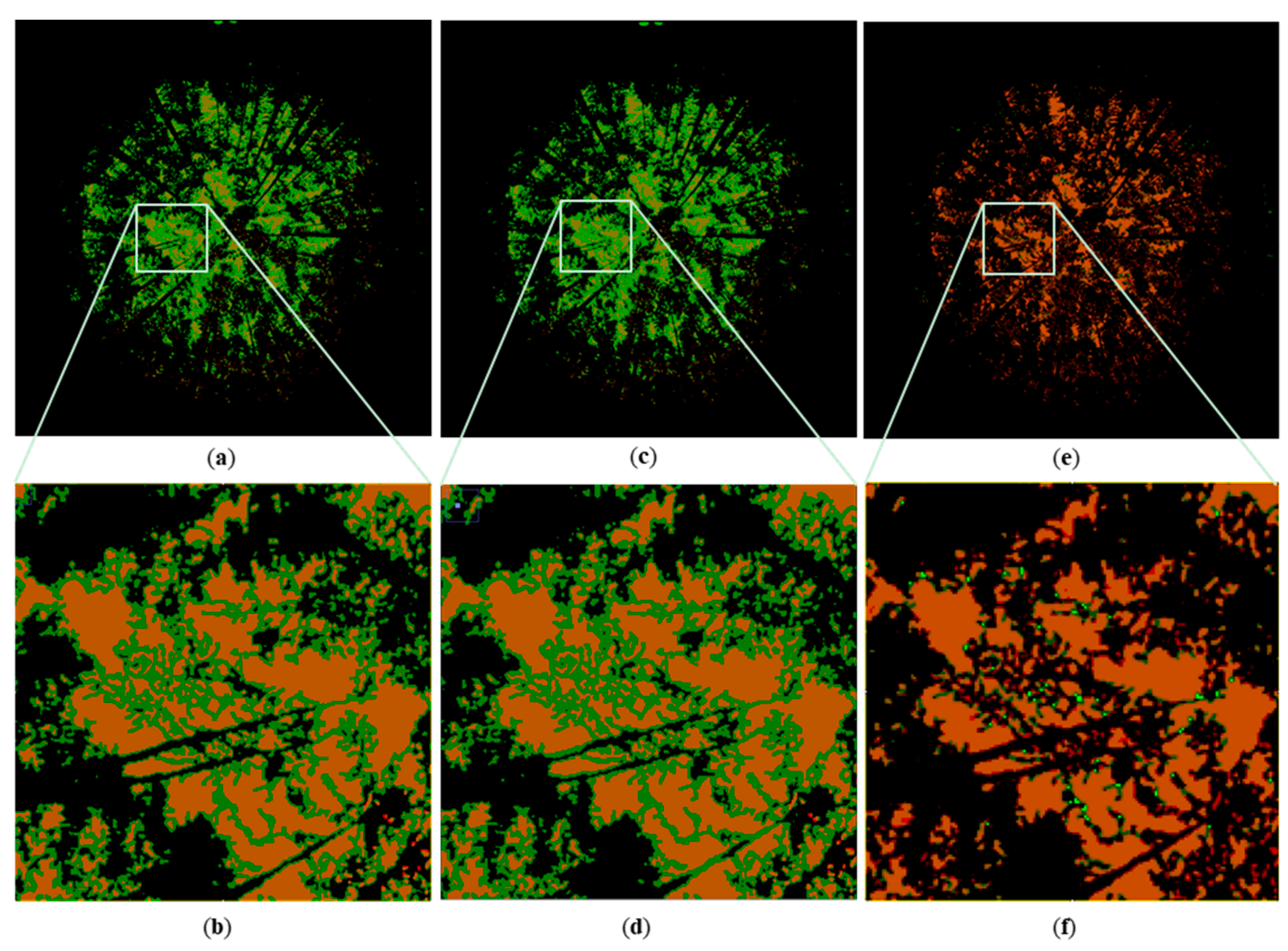
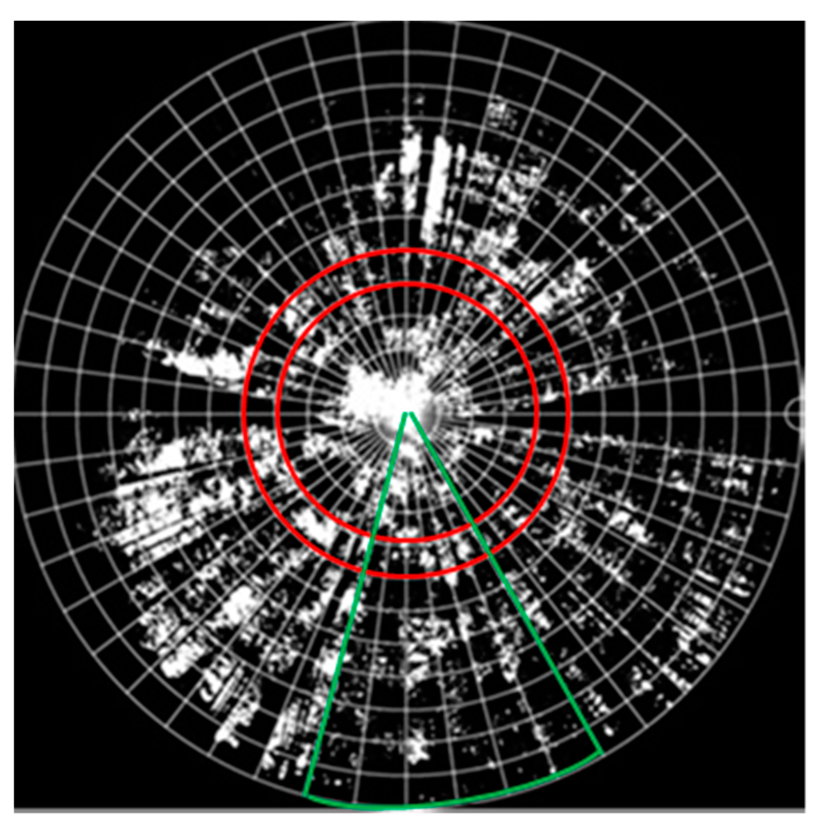
Our method also has limitations. One of the limitations is that producing the manual reference images is time consuming and laborious. As the size of the canopy hemisphere image is large (2736 × 2736), and the boundaries between the sky and the vegetation are blurred, it is difficult for human vision to distinguish them, and it will take a large amount of time to delineate the sky and vegetation pixels manually. To solve this problem, we can adopt an alternative training strategy based on image patches. That is, the canopy hemisphere image can be divided into subregions (sectoral or circular regions) according to the symmetry axis of the image, as shown in Figure 12. The region surrounded by the green line is a sector subregion, and the two red circles form a ring. The circular image is divided into sky pixels (presented in white color) and vegetation pixels (presented in black color), that is, the sky and vegetation are classified as two categories. If we only train the image patches (sectors or rings), this can greatly reduce the time spent finding the manual reference images.

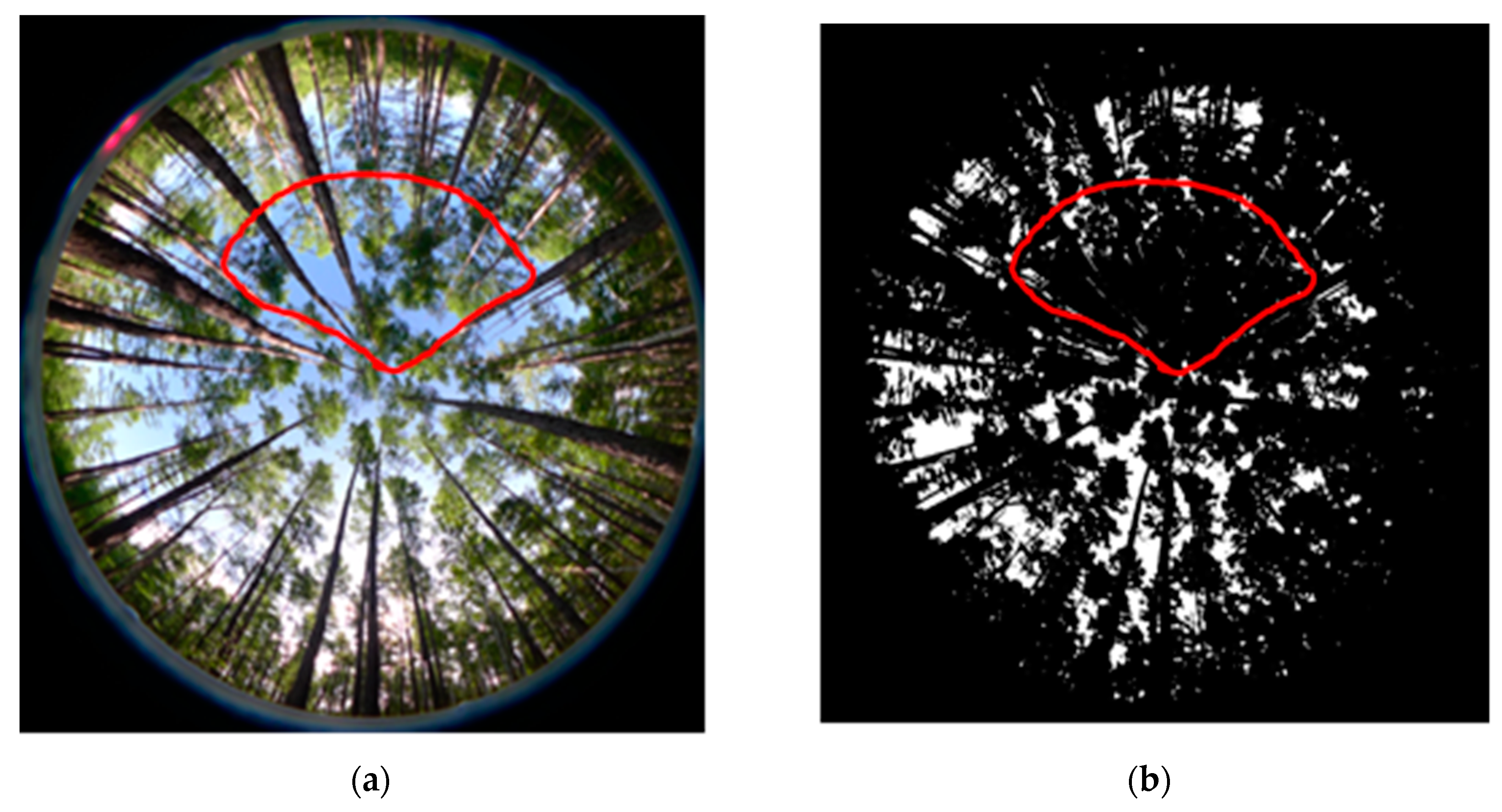
The second limitation is that the generalization ability of our method still needs to be improved. Generally speaking, it is recommended that hemispherical canopy images are taken in dawn, twilight, or overcast conditions [24,25]. Unfortunately, some of the data we obtained were collected under sunny or cloudy conditions, and the acquired image quality was not ideal. For this reason, when performing the algorithm experiments, we removed all data with direct sunlight; however, for the canopy images with a blue sky background, our method provides incorrect segmentation results, where the blue sky is wrongly divided into vegetation, as shown in Figure 13. Although, this image was taken from another data set (which captured in 2014) and was not included in our experiments. The blue sky in the area surrounded by the red line was identified as vegetation (shown in black, see Figure 13b). The reason for this may be that our training dataset contained few images with blue sky, which has affected the generalization ability of the model. In fact, from an ecological perspective, the CHP images should be taken in overcast conditions, and images with blue sky are not suitable.

In addition, the main research objects of this paper were coniferous forests and mixed forests. These two types of canopy hemisphere images often contain small gaps (the light-transmitting part between the branches and leaves) as the small foliage and leaves are weakly contrasted against the sky background, where the identification of these small gaps thus belongs to small object segmentation. The U-Net model has poor segmentation performance for small object segmentation [21]. Subsequent research can attempt to use R-CNN mask to segment canopy hemisphere images.

Another factor that affects the performance of our method is the exposure mode. The auto exposure mode was used in our experiments, because this setting is convenient and can save a lot of data collection time. However, some research suggests manual exposure mode for hemispherical data collection [24,25]. Using auto exposure as a reference, the lower exposure is suitable for dense canopies, and a higher exposure is suitable for sparse canopies. In future studies, we will try to use the manual mode.

The forest canopy image segmentation results can be used to calculate the GF of the canopy. These GF values can be combined with different canopy models to provide LAI values. The LAI is one of the most important parameters for describing the characteristics of forest canopy structure, and it is also an important factor explaining differences in net primary productivity above the ground. The LAI of the canopy determines the light, temperature, and humidity in a forest, thereby affecting the balance of carbon, water, and energy. It is usually used to characterize the structure and functional characteristics of the forest ecosystem. Overall, the canopy hemisphere image segmentation method proposed in this paper is of great significance for the accurate estimation of forest LAI values and provides technical support for forest ecology research.

5. Conclusions

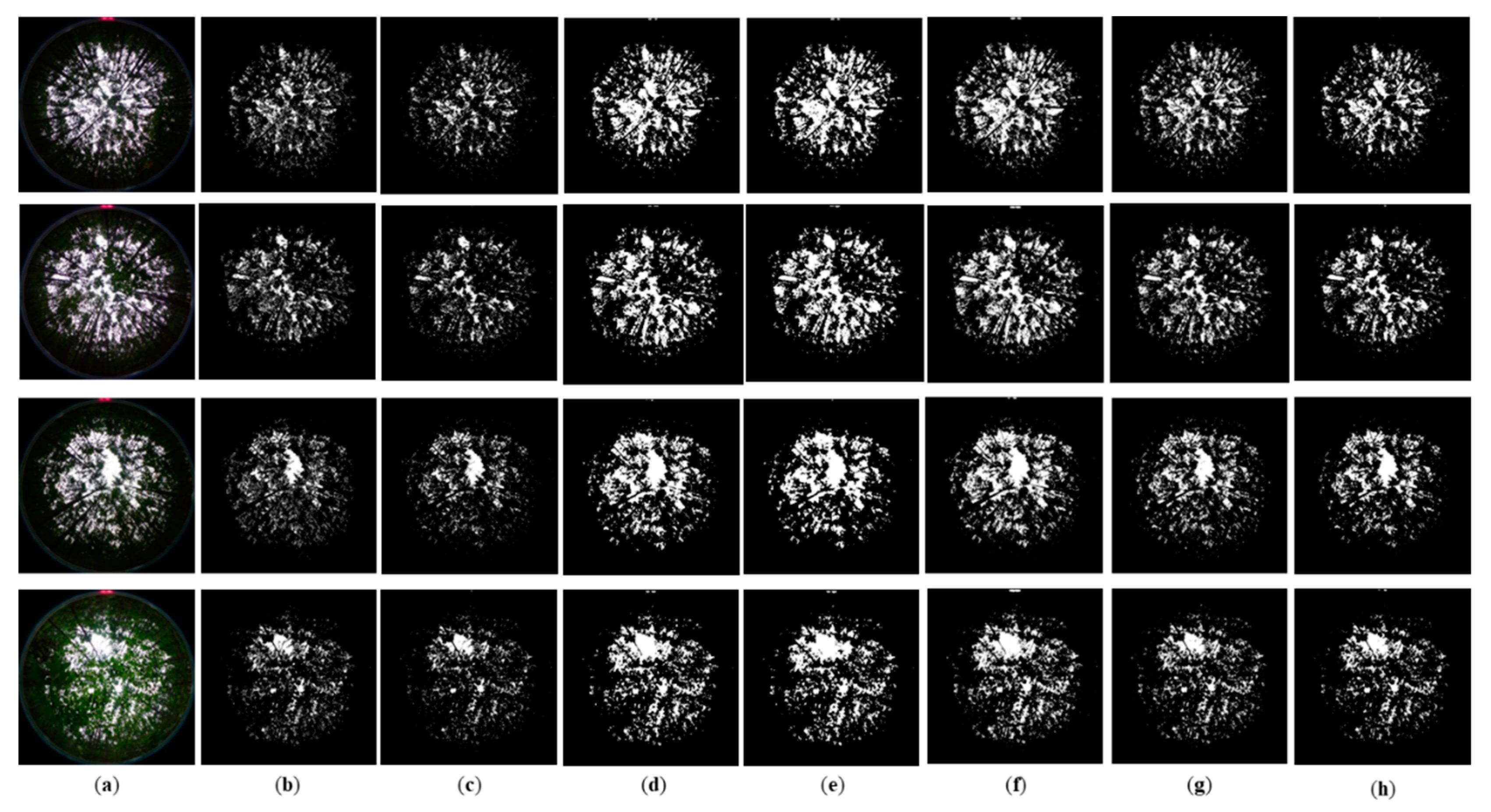
This paper has proposed a new method for forest CHP segmentation based on deep learning technology. The method includes three steps, namely, northing correction, valid region extraction, and canopy images segmentation. This method takes the original CHP image as an input and outputs canopy image segmentation results. The whole process of image processing does not require manual intervention and is an end-to-end and fully automatic method. Through the experiments with CHP images of Korean pine and mixed forests, our method achieved a DSC of 89.20% and an accuracy of 98.73% for CHP segmentation. Compared with the Habitat-Net model, the WinSCANOPY professional software, a clustering method, and traditional threshold methods (i.e., the Otsu and Ridler methods), our method achieved the best segmentation results. It only requires about 1 s for taking the original canopy images (2736 × 2736) and outputting the binary segmentation results, and the algorithm has been shown to be efficient. This method can support the estimation of forest canopy GF and LAI values.

References

1. Dezhi, L. The research advances on the structure and function of forest canopy, as well as their temporal and spatial changes. World Forest. Res. 2004, 17, 12–16. [Google Scholar]
2. Rautiainen, M.; Mottus, M.; Heiskanen, J.; Akujarvi, A.; Majasalmi, T.; Stenberg, P. Seasonal reflectance dynamics of common understory types in a northern European boreal forest. RSE 2011, 115, 3020–3028. [Google Scholar] [CrossRef]
3. Lee, Y.J.; Alfaro, R.I.; Sickle, G.A.V. Tree-crown defoliation measurement from digitized photographs. Can. J. Forest Res. 1983, 13, 956–961. [Google Scholar] [CrossRef]
4. Leblanc, S.G.; Chen, J.M.; Fernandes, R.; Deering, D.W.; Conley, A. Methodology comparison for canopy structure parameters extraction from digital hemispherical photography in boreal forests. Agric. Forest Meteorol. 2005, 129, 187–207. [Google Scholar] [CrossRef] [Green Version]
5. Ishida, M. Automatic thresholding for digital hemispherical photography. Can. J. Forest Res. 2004, 34, 2208–2216. [Google Scholar] [CrossRef]
6. Juárez, R.I.N.; Rocha, H.R.D.; Figueira, A.M.S.E.; Goulden, M.L.; Miller, S.D. An improved estimate of leaf area index based on the histogram analysis of hemispherical photographs. Agric. Forest Meteorol. 2009, 149, 920–928. [Google Scholar] [CrossRef] [Green Version]
7. Macfarlane, C. Classification method of mixed pixels does not affect canopy metrics from digital images of forest overstorey. Agric. Forest Meteorol. 2011, 151, 833–840. [Google Scholar] [CrossRef]
8. Mizoue, N.; Inoue, A. Automatic thresholding of tree crown imagesautomatic thresholding of tree crown images. J. For. Plann. 2001, 6, 75–80. [Google Scholar]
9. Jonckheere, I.; Nackaerts, K.; Muys, B.; Coppin, P. Assessment of automatic gap fraction estimation of forests from digital hemispherical photography. Agric. Forest Meteorol. 2005, 132, 96–114. [Google Scholar] [CrossRef]
10. Inoue, A.; Yamamoto, K.; Mizoue, N. Comparison of automatic and interactive thresholding of hemispherical photography. J. Forest Sci. 2011, 57, 78–87. [Google Scholar] [CrossRef] [Green Version]
11. Glatthorn, J.; Beckschäfer, P. Standardizing the protocol for hemispherical photographs: Accuracy assessment of binarization algorithms. PLoS ONE 2014, 9, e111924. [Google Scholar] [CrossRef] [PubMed] [Green Version]
12. Woodgate, W.; Disney, M.; Armston, J.D.; Jones, S.D.; Suarez, L.; Hill, M.J.; Wilkes, P.; Soto-Berelov, M.; Haywood, A.; Mellor, A. An improved theoretical model of canopy gap probability for leaf area index estimation in woody ecosystems. Forest Ecol. Manag. 2015, 358, 303–320. [Google Scholar] [CrossRef]
13. Nobis, M.; Hunziker, U. Automatic thresholding for hemispherical canopy-photographs based on edge detection. Agric. Forest Meteorol. 2005, 128, 243–250. [Google Scholar] [CrossRef]
14. Pueschel, P.; Buddenbaum, H.; Hill, J. An efficient approach to standardizing the processing of hemispherical images for the estimation of forest structural attributes. Agric. Forest Meteorol. 2012, 160, 1–13. [Google Scholar] [CrossRef]
15. Diaz, G.M.; Lencinas, J.D. Enhanced gap fraction extraction from hemispherical photography. IEEE Geosci. Remote Sens. Lett. 2015, 12, 1784–1789. [Google Scholar] [CrossRef]
16. Huang, Q.Y.; Fan, X.L.; Zhang, M.; Huang, X.; Li, P.; FU, H.T.; Tang, S.H. Comparative study of image segmentation algorithms for rice canopy. Chin. J. Eco-Agric. 2018, 26, 710–718. [Google Scholar]
17. Zhao, T.; Yang, Y.; Niu, H. Comparing U-Net convolutional network with mask R-CNN in the performances of pomegranate tree canopy segmentation. In Proceedings of the Conference on Multispectral, Hyperspectral, and Ultraspectral Remote Sensing Technology, Techniques, and Applications, Honolulu, HI, USA, 24–26 September 2018. [Google Scholar]
18. Wagner, F.H. Using the U-net convolutional network to map forest types and disturbance in the Atlantic rainforest with very high resolution images. Remote Sens. Ecol. Conserv. 2019, 5, 360–375. [Google Scholar] [CrossRef] [Green Version]
19. Abrams, J.F.; Vashishtha, A.; Wong, S.T.; Nguyen, A.; Mohamed, A.; Wieser, S.; Kuijper, A.; Wilting, A.; Mukhopadhyay, A. Habitat-Net: Segmentation of habitat images using deep learning. Ecol. Informa. 2019, 51, 121–128. [Google Scholar] [CrossRef]
20. Wang, D.; Cui, H.; Chen, J. Improvement of fisheye image edge extraction algorithm. Comp. Eng. Des. 2007, 28, 2878–2882. [Google Scholar]
21. Ronneberger, O.; Fischer, P.; Brox, T. U-Net: Convolutional networks for biomedical image segmentation. In Proceedings of the International Conference on Medical Image Computing and Computer-Assisted Intervention, Munich, Germany, 5–9 October 2015; Springer: Cham, Switzerland, 2015; pp. 234–241. [Google Scholar]
22. Zhang, N.; Shelhamer, E.; Gao, Y.; Darrell, T. Fine-grained pose prediction, normalization, and recognition. arXiv 2015, arXiv:1511.07063. [Google Scholar]
23. Taha, A.A.; Hanbury, A. Metrics for evaluating 3D medical image segmentation: Analysis, selection, and tool. BMC Med. Imag. 2015, 29, 8–12. [Google Scholar] [CrossRef] [PubMed] [Green Version]
24. Zhang, Y.; Chen, J.M.; Miller, J.R. Determining digital hemispherical photograph exposure for leaf area index estimation. Agric. Forest Meteorol. 2005, 133, 166–181. [Google Scholar] [CrossRef]
25. Díaz, G.M.; Lencinas, J.D. Model-based local thresholding for canopy hemispherical photography. Can. J. Forest Res. 2018, 48, 1204–1216. [Google Scholar] [CrossRef]
Figure 1. The principle of canopy hemispherical photography (CHP).
Forests 11 01366 g001
Figure 2. Overall flow chart of the canopy segmentation method.
Forests 11 01366 g002
Figure 3. The site of the Mengjiagang Forest Farm.
Forests 11 01366 g003
Figure 4. The principle of the scanning algorithm and the valid region. (a) Algorithm interpretation; (b) valid region shown by the red circle.
Forests 11 01366 g004
Figure 5. Proposed U-Net architecture.
Forests 11 01366 g005
Figure 6. Illustration of evaluation metrics for image segmentation.
Forests 11 01366 g006
Figure 7. Comparison of segmentation results for six different methods: (a) Original canopy hemispherical photography (CHP) images; (b) manually extracted reference images, segmentation results obtained from (c) newly developed U-net method as well as from (d) Otsu; (e) Ridler; (f) fuzzy clustering method (FCM); (g) WinSCANOPY; (h) Habitat-Net methods.
Forests 11 01366 g007
Figure 8. Overlay details for different methods: (a) Overlay of Otsu and manual reference images; (b) local enlargement of (a); (c) overlay of Ridler and manual reference images; (d) local enlargement of (c); (e) overlay of U-net and manual reference images; (f) local enlargement of (e).
Forests 11 01366 g008
Figure 9. Local detail comparison of a mixed forest canopy (small foliage in the green circles under heavy sunlight). (a) Original CHP images; (b) manually extracted reference images, segmentation results obtained from (c) newly developed U-net method as well as from (d) Otsu; (e) Ridler; (f) fuzzy clustering method (FCM); (g) WinSCANOPY; (h) Habitat-Net methods.
Forests 11 01366 g009
Figure 10. Coniferous forest (Korean pine) canopy local detail comparison (small foliage in the green circles under heavy sunlight). (a) Original CHP images; (b) manually extracted reference images, segmentation results obtained from (c) newly developed U-net method as well as from (d) Otsu; (e) Ridler; (f) fuzzy clustering method (FCM); (g) WinSCANOPY; (h) Habitat-Net methods.
Forests 11 01366 g010
Figure 11. Accuracy and loss curves for the training process.
Forests 11 01366 g011
Figure 12. Subregion divisions of the CHP.
Forests 11 01366 g012
Figure 13. The segmentation result of the canopy image containing the blue sky. (a) Original image; (b) segmented image by our method.
Forests 11 01366 g013