Evaluating Street Greenery by Multiple Indicators Using Street-Level Imagery and Satellite Images: A Case Study in Nanjing, China

Abstract

Street greenery plays an essential role in improving the street environment and residents’ health. The evaluation of street greenery is of great value to establish environmentally friendly streets. The evaluation indicators of present studies evaluating street greenery were relatively single, either the Green View Index (GVI) or Normalized Difference Vegetation Index (NDVI), which cannot describe the greenery condition in its entirety. The objective of this study is to assess the street greenery using multiple indicators, including GVI, NDVI, and Vegetation Structural Diversity (VSD). We combined street view images with a semantic segmentation method to extract the GVI and VSD and used satellite images to calculate the NDVI in the urban area of Nanjing, China. We found correlations and discrepancies of these indicators using statistical analyses in different urban districts, functional areas, and road levels. The results indicate that: (1) the GVI and NDVI are strongly correlated in open spaces, whereas weakly correlated in residential and industrial lands, (2) the areas with higher VSD are mainly located in the new city, whereas the VSD in the old city is lower, and a weak negative correlation exists between the GVI and VSD in the research area, and (3) the old city has a higher GVI level compared to the new city on the main road, whereas the new city has a higher GVI level than the old city on the branch road. Compared with the GVI, the trend of VSD in the old city and the new city is relatively consistent. Our findings suggest that considering multiple indicators of street greenery evaluation can provide a comprehensive reference for building more human-friendly and diversified street green belts.

1. Introduction

Street greenery plays a significant role in improving the urban street environment and public health. The trees with large crowns, leaves and branches or the combination of trees and shrubs [1] can make a “green wall” to reduce the noise by blocking the transmission of sound waves [2]. Moreover, the street vegetation can decrease the heat island effect through shading and evapotranspiration [3,4] and remove air pollutants through the dry deposition process [5] and stomatal absorption [2], especially with broadleaf species [5]. In addition, street greenery can also improve the odds of residents participating in physical activity [6,7,8], decrease the obesity rate [8] and enhance mental wellbeing [9,10]. Some researchers found that street greenery has a positive relationship with housing prices [10], personal income [11] and is negatively associated with the crime rate [12]. Therefore, a quantitative measurement of street greenery is beneficial for establishing environmentally friendly streets.

Available data sources used to evaluate street greenery include on-site photographs, street view images, remote sensing images and three-dimensional point cloud data. The on-site photos are taken by the camera, and the green vegetation is outlined by image processing software to evaluate the green view index (GVI) [13], an index initially proposed by Aoki [14] that measures the greenery from the perspective of pedestrians (eye-level greenery). However, the collecting and processing of the photos are time-consuming and labor-intensive [15]. In comparison, remote-sensing images are collected by satellites and are easy to download or purchase online, and vegetation evaluation indices based on remote-sensing images is widely used, such as the Normalized Difference Vegetation Index (NDVI) [16]. However, remote-sensing images can only be used to evaluate overhead greenery, which is different from the eye-level greenery that pedestrians perceive on the ground [17,18].

On the contrary, street view images can be used to evaluate eye-level greenery. Compared with field photos, the street view images have broader coverage and lower costs to obtain [19]. The shooting height of the street view image is close to the height of the human line of sight [20], and the street view image will not omit the information of undergrowth vegetation, such as shrubs and grasslands [18,20], which can better reflect the human visual feeling of street greening. At present, street view images have been widely used in the evaluation of urban street environments, such as urban landscape evaluations [21,22], human visual perception evaluations [9,23] and walkability evaluations [24,25]. Besides, point cloud data can also be used in greenery assessments [26], but the cost of data acquisition is high.

Plenty of automatic methods have been proposed to extract vegetation based on street view images, such as band operation [20], color space conversion [15,27], support vector machine [28] and image semantic segmentation [7,29]. Compared with the first three methods based on color space, which may confuse vegetation and other manmade green features [20], the image semantic segmentation method can achieve a satisfactory accuracy level and separate vegetation from other green objects. Furthermore, the influence of season variations on its accuracy level is mild, because its recognition mechanism does not rely on color but, instead, relies on object features.

Many previous studies assessed street greenery in one perspective: overhead greenery by satellite images or eye-level greenery by street view images. However, few studies have assessed greenery comprehensively in two perspectives. Ye et al. [29] and Lu et al. [17] compared eye-level greenery and urban green cover using remote sensing at the regional level; thus, street-level differences between eye-level greenery and overhead greenery are still unexplored.

The present studies on evaluating street greenery with street view images have only measured the amount of greenery, without distinguishing upper and lower greenery. As a part of the urban forest, street greening has a vertical structure similar to the forest community. The vertical structure of the forest community is divided into four essential layers based on their growth habits: tree layer, shrub layer, herb layer and ground cover layer. The shrub, herb and ground cover layers are collectively called understory vegetation [30]. The understory vegetation has the highest biodiversity among plants and provides habitat for many animals [31]. Additionally, understory vegetation contributes to nutrient cycling and tree growth [30] and plays a positive role in maintaining the soil surface’s stability [32]. For pedestrians, a wide variety of understory species can make the street landscape more attractive and promote social activities [32]. Thus, it is misleading for planners to only aim to increase street tree coverage but neglect shrubs and herbs [33]. Compared to single-layer structures, residents prefer denser and more complex urban vegetation structures [34], such as trees planted over shrubs, which have aesthetic benefits, and trees planted over turf grass, which improve the air quality as well as mental wellbeing [35]. A combination of trees and understory vegetation can better support biodiversity and ecosystem services than trees or shrubs alone [31,35]. Therefore, it is necessary to measure the complexity of street-side vegetation structures to improve the biodiversity and beauty of urban green spaces.

The main objective of this study was to evaluate the street greenery using multiple indicators by street-level imagery and satellite images. A new indicator, street vegetation structural diversity (VSD), was proposed to measure the diversity of trees, shrubs and herbs. To achieve this, we used Nanjing City to explore the detailed distribution patterns of street greenery and their associations with urban functional zones (UFZs) and road levels. Furthermore, a multi-perspective analysis of the street greenery was presented to explore the relationship between the GVI and NDVI. The assessment results can provide reference for further studies and can be used to develop planning practices for urban street greenery designs.

2. Materials and Methods

2.1. Study Area

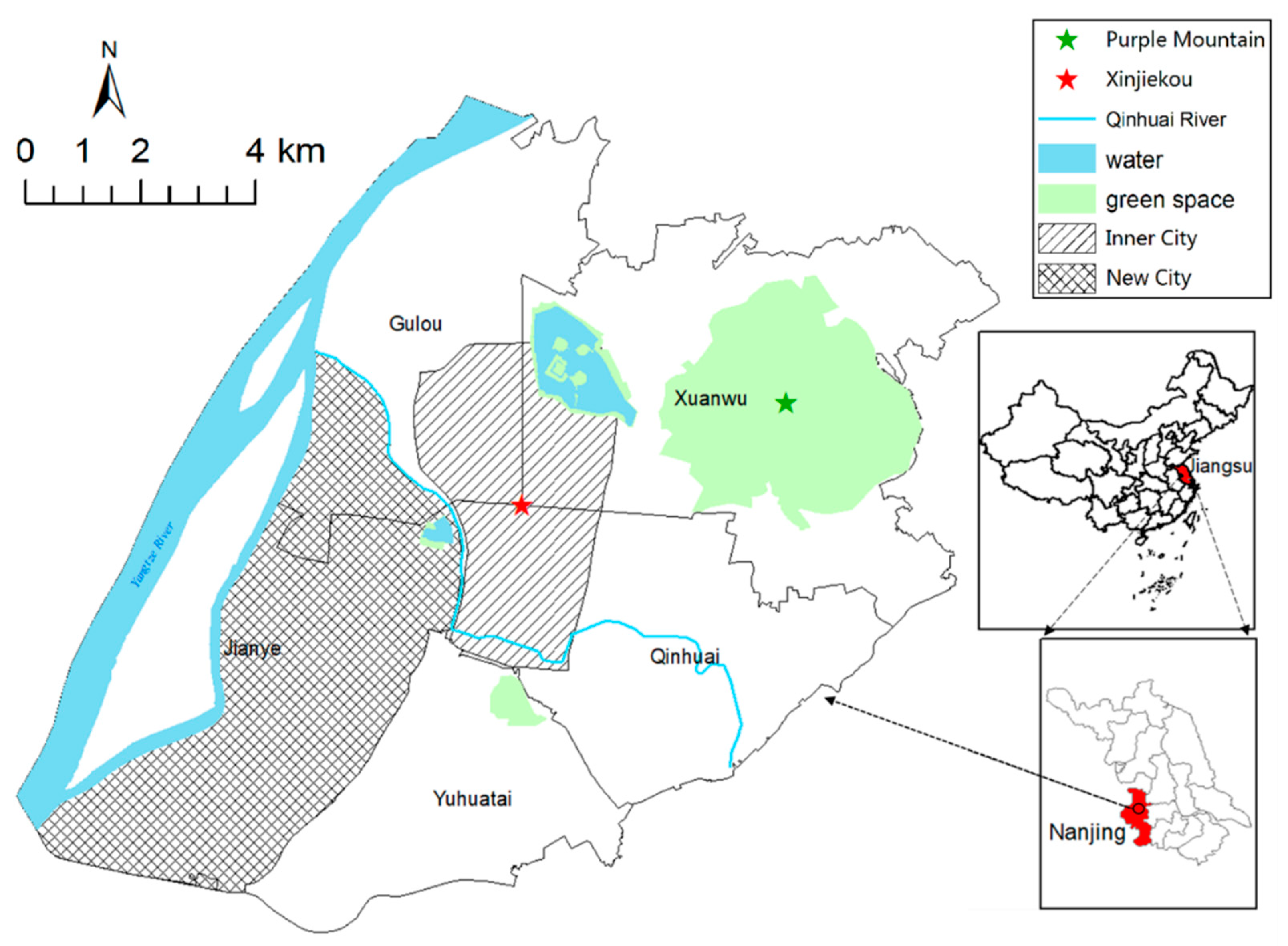
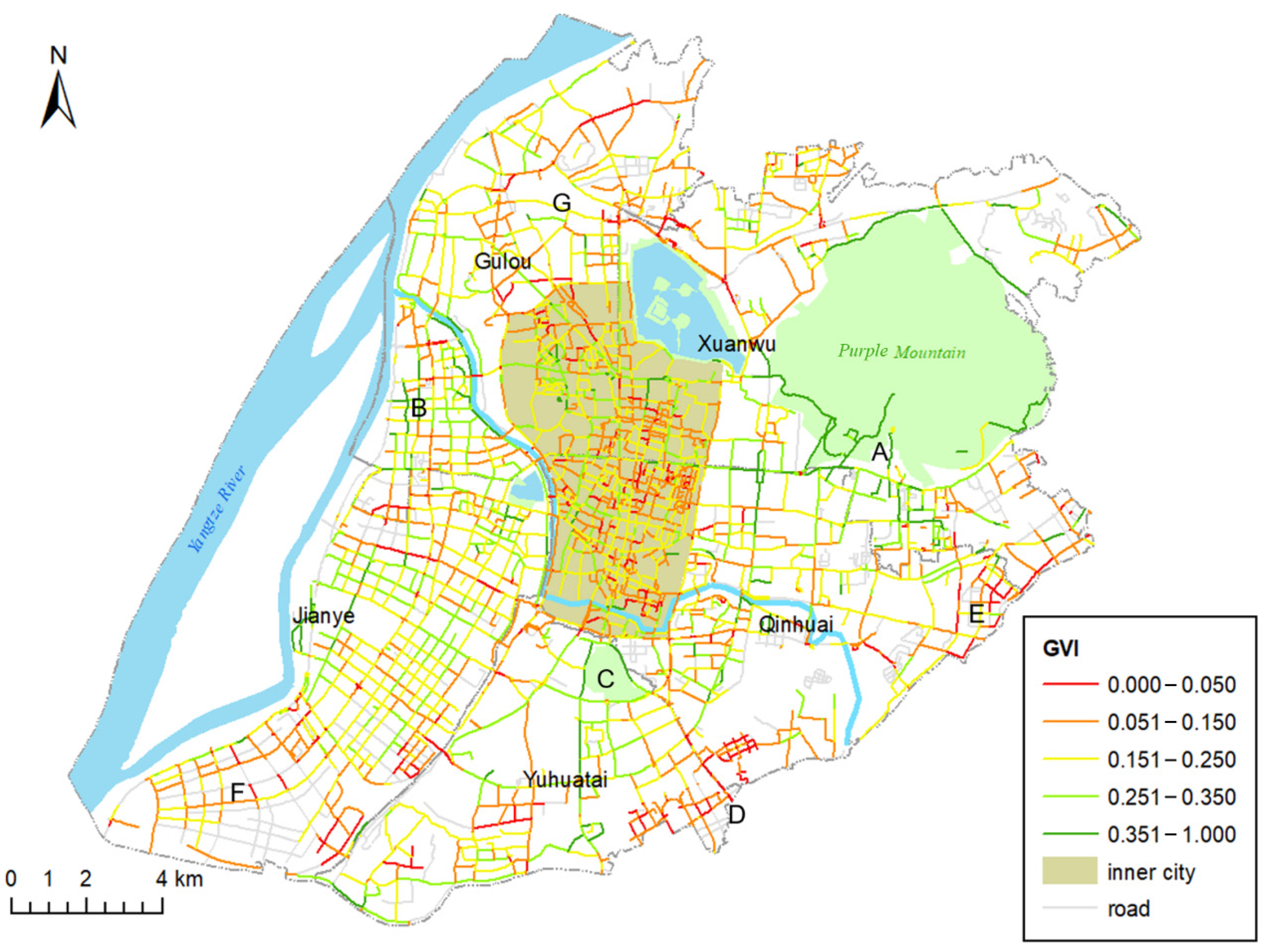
The research was conducted in Nanjing, a city located in the Yangtze River Delta region of Eastern China, which consists of 9 urban districts and two suburban districts. The city has a northern subtropical humid climate and has abundant rainfall in the summer. The population of Nanjing is nearly 8.5 million, and its administrative area is about 6600 km². Unlike many megacities in China like Beijing and Shanghai, Nanjing urban areas are situated within the natural landscape and include Purple Mountain, Xuanwu Lake, Yangtze River, and Qinhuai River (Figure 1). The present studies related to the street greenery assessment in China have mainly focused on Beijing and Shanghai [27,36,37] or one administrative district of Nanjing [38], whereas the entire urban area of Nanjing is still unexplored.

Therefore, we selected the urban area of Nanjing as the study area, which includes five administrative districts: Gulou, Xuanwu, Jianye, Qinhuai and the northern part of Yuhuatai.

2.2. Data Preprocessing

The road network in the research area was downloaded from OpenStreetMap (OSM), a map platform that can be edited by every user and provides free geodata, including road networks, building footprints and points of interest. 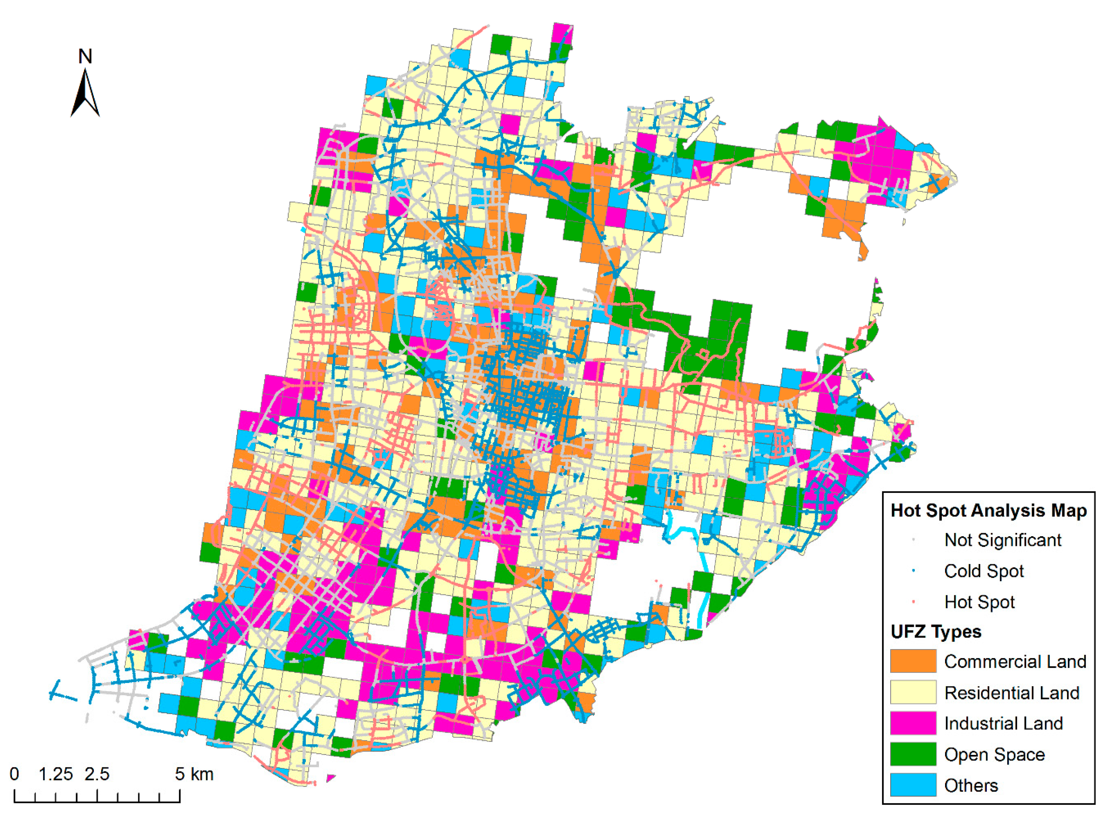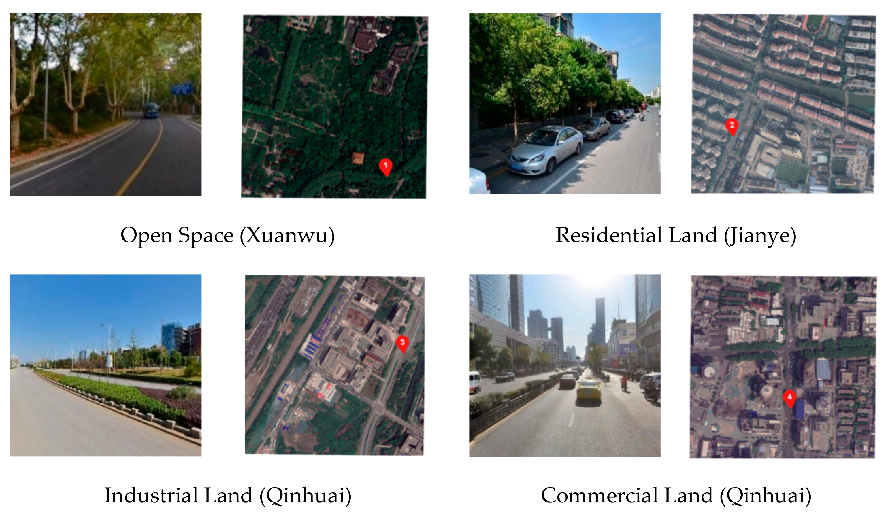Street view images were downloaded from the Tencent Street View (TSV) service, and the satellite images used were Landsat 8 images taken in October 2013 with a 30-m resolution, downloaded from the Geospatial Data Cloud (http://www.gscloud.cn). The UFZ data were collected from [39], which divides the urban area into several grids of 500 m × 500 m, and each grid corresponds to an urban functional type. The urban functional type and grid number of each type are shown in

Table 1. Urban functional zone (UFZ) types and grid numbers of each type.

Type	Commercial Land	Residential Land	Industrial Land	Open Space	Others
Number	136	415	131	94	90
Proportion	15.7%	47.9%	15.1%	10.9%	10.4%

, of which open space contains parks, scenic spots and other large open areas.

Since the OSM road data contained some topological and geometrical errors, several steps were needed for road network refinement, and the workflow was as follows:

• Determination of the road level: Six levels of the road were selected from the OSM data according to the “highway” attribute, including the trunk, primary, secondary, tertiary, residential and living streets. Since the road level classification criterion was not consistent with that used in China, which classifies roads into four categories: expressway, main road, secondary road and branch road, the authors made a corresponding relationship between two classification criteria (

  Table 2. The corresponding relationship between the OpenStreetMap (OSM) road level and the Chinese road level. The road count and the range of road widths of each road level are also listed.

  OSM Road Level	Chinese Road Level	Road Count	Width
  Trunk	Trunk road	291	50–65 m
  Primary	Major road	787	40–50 m
  Secondary	Minor road	778	24–40 m
  Tertiary	Minor road
  Residential	Branch road	2491	$\le 24\mathrm{m}$
  Living street	Branch road

  ) and made the road level comply with the Chinese criterion.
• Modification of the road geometry: In the road network data, there is a gap between the position of some road segments and the actual positions of the road, which needs to be adjusted manually. The Tencent map was used as a reference for road geometry adjustments, and some large inconsistencies were modified.
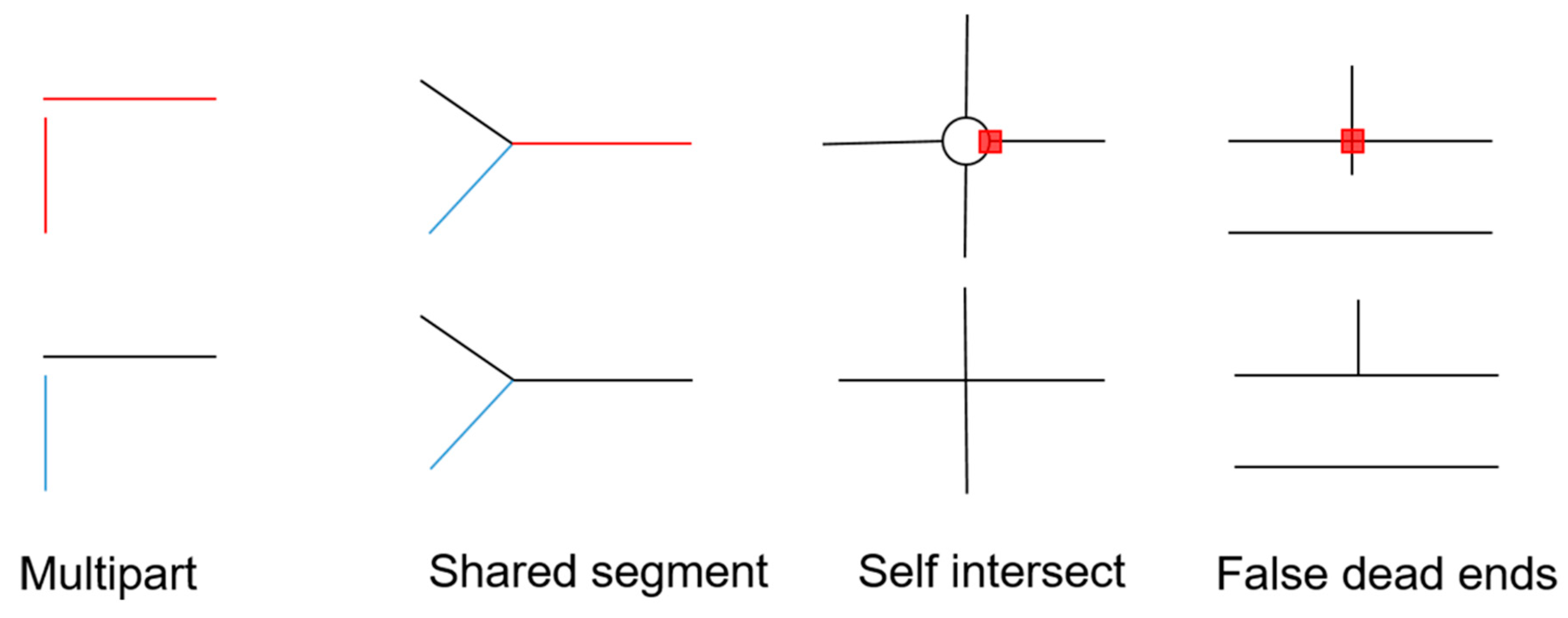
• Editing of the topology: Some topology errors, including false dead ends, multipart geometries, self-intersects and shared geometries in the road network, might affect the results of the road merging process. Multipart geometries were separated by the “multipart to single part” tool in ArcGIS, and other errors were fixed manually (Figure 2).
• The merging of multilane roads: Some roads have multiple lanes and complex structures such as viaducts and tunnels, which, in some cases, caused the locations of street view images to be inconsistent with the corresponding lane. Therefore, the “merge divided roads” tool was used to merge the road lanes into a single line.
• Generation of sample sites: In order to get street view images by coordinates, sample sites were generated, along with the road network, in 50-m intervals, following previous studies [26], and then, coordinates of the points were calculated in the WGS-84 coordinate system.

2.3. Extracting Vegetation from TSV Images

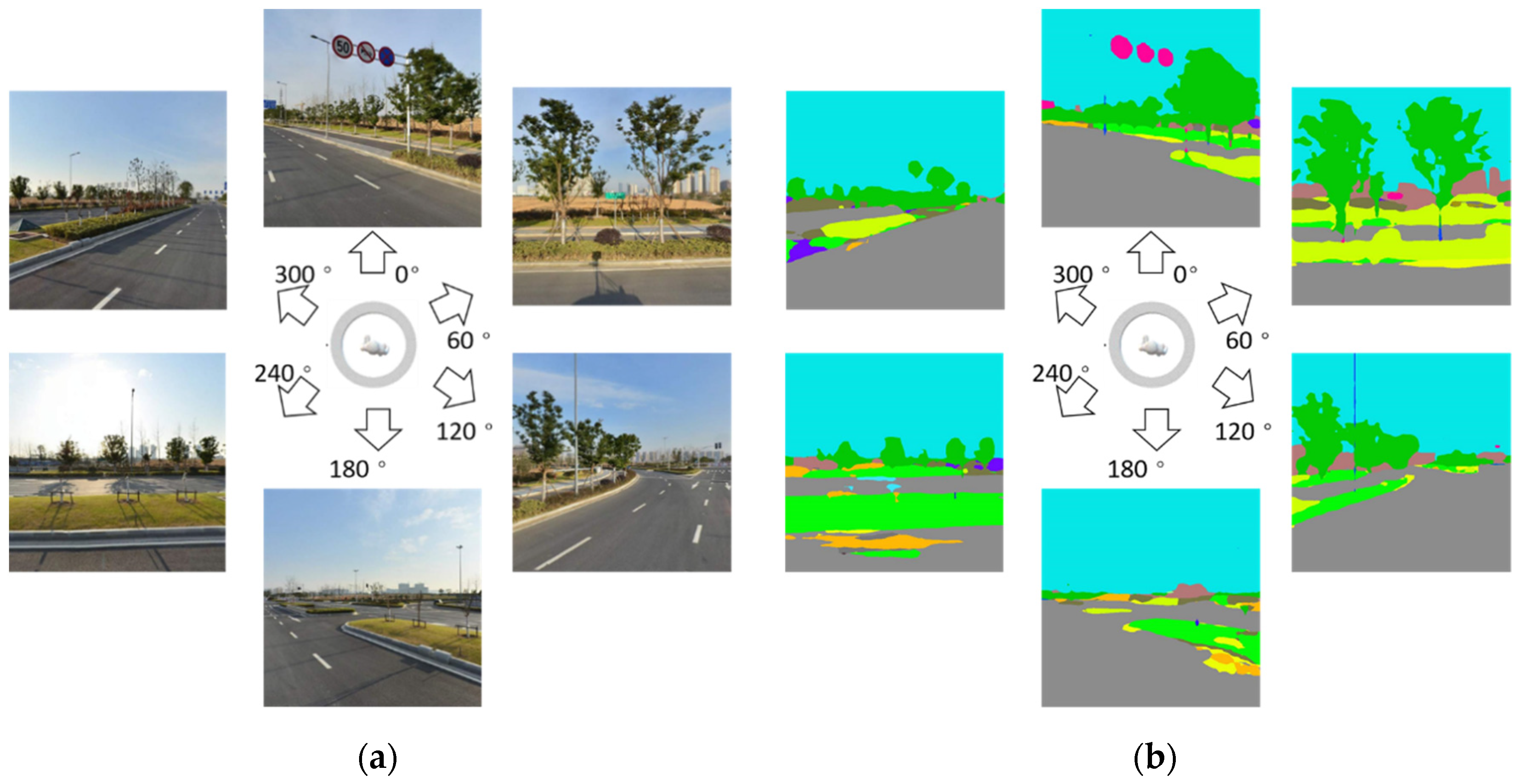
Several companies provide online street-view downloading services, and the TSV was chosen for its high image quality and wide coverage of images. The service provides an Application Program Interface (API) for users to download images by passing on a series of parameters, including the location, panoramic ID (panoid), image width, image height, heading, pitch and key. The meanings of the parameters are explained in

Table 3. Explanation of some parameters in the street view Application Program Interface (API).

Parameter	Explanation
Panoid	A unique ID of a panorama.
Heading	The horizontal angle between the camera and north direction. Range: (0–360)
Pitch	The vertical angle of the camera. Range: (−20–90)
Key	The key provided for registered developers.

. The workflow used to obtain the images included the following steps. Firstly, the coordinates of the sample sites were transformed into the coordinates of the Tencent Map. Secondly, panoids were obtained by requesting the “scene information query” API through coordinates. Thirdly, the “street view static image query” API was requested in 6 directions to get 6 street view images of the point (Figure 3a). The example Uniform Resource Locator (URL) is as follows (The key value should be replaced with the key applied by registered developers):

https://apis.map.qq.com/ws/streetview/v1/image?size=600x600&pano=10011022120723095812200&pitch=0&heading=0&key=OB4BZ-D4W3U-B7VVO-4PJWW-6TKDJ-WPB77.

For each site, the size was set as 600 × 600 (px), the pitch was set to 0 (degree) and the headings were set as 0, 60, 120, 180, 240 and 300 (degrees), respectively.

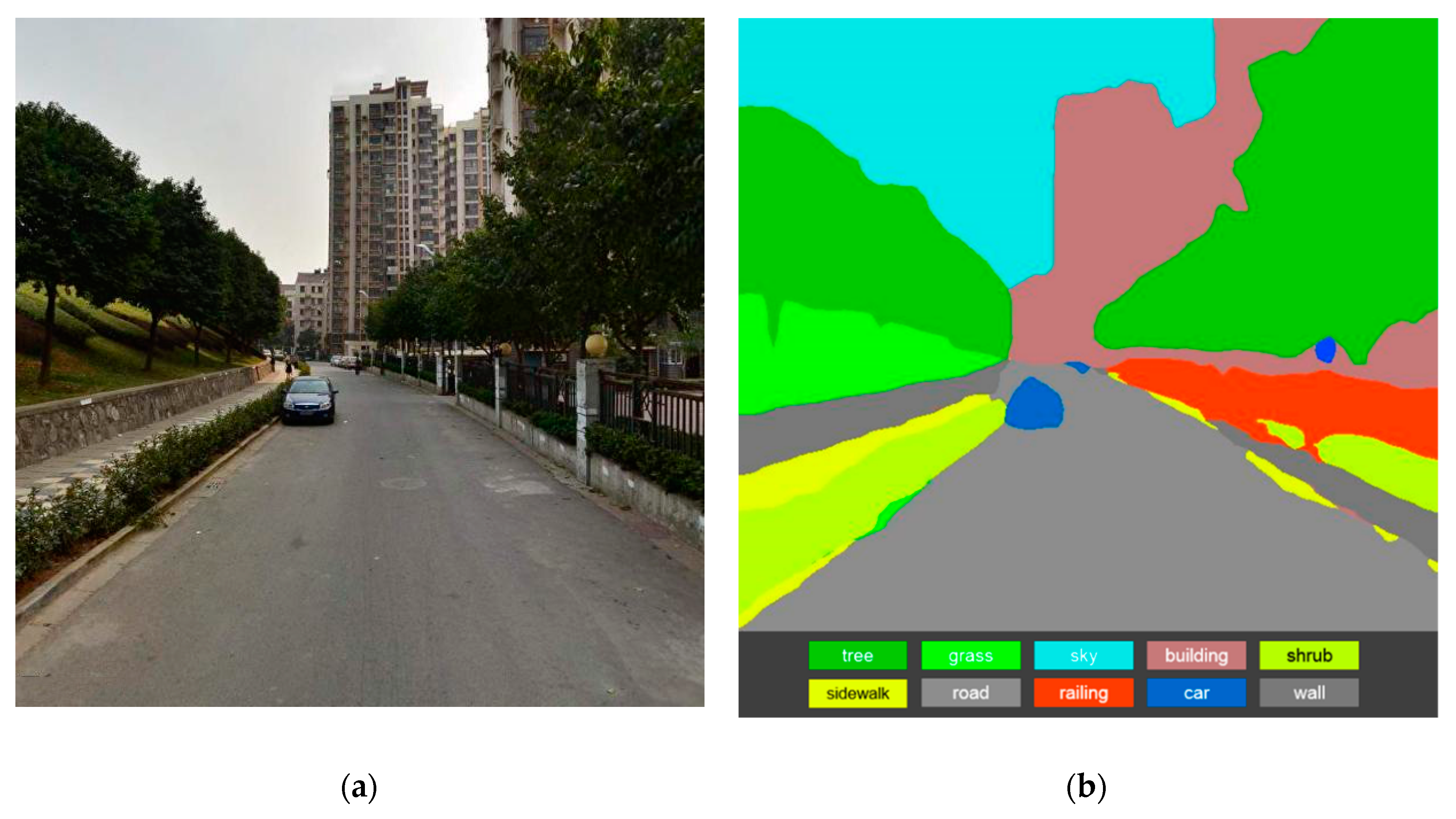
In order to calculate the GVI of each site, the pixels of vegetation needed to be identified from the street view images (Figure 3b). A semantic segmentation framework, Pyramid Scene Parsing Network (PSPNet), was used to extract vegetation from images. This framework can accomplish pixel-level prediction tasks and achieve state-of-the-art performances on various datasets [40]. It uses a Convolutional Neural Network (CNN) to extract the features of the image and a pyramid pooling module to obtain different scales of feature representations. After the process of upsampling and concatenation, the final prediction is output from the last convolutional layer. With the picture fed into, the network predicts each image pixel category, such as tree, sky or building. Here, we used a pretrained model on the labeled dataset ADE20K [41] and made predictions on all images. An example of a segmentation result by PSPNet is shown in Figure 4. In this picture, different vegetation types are distinguished, making it possible to analyze the vegetation composition and diversity.

2.4. Assessing Street Greenery through Multiple Indicators

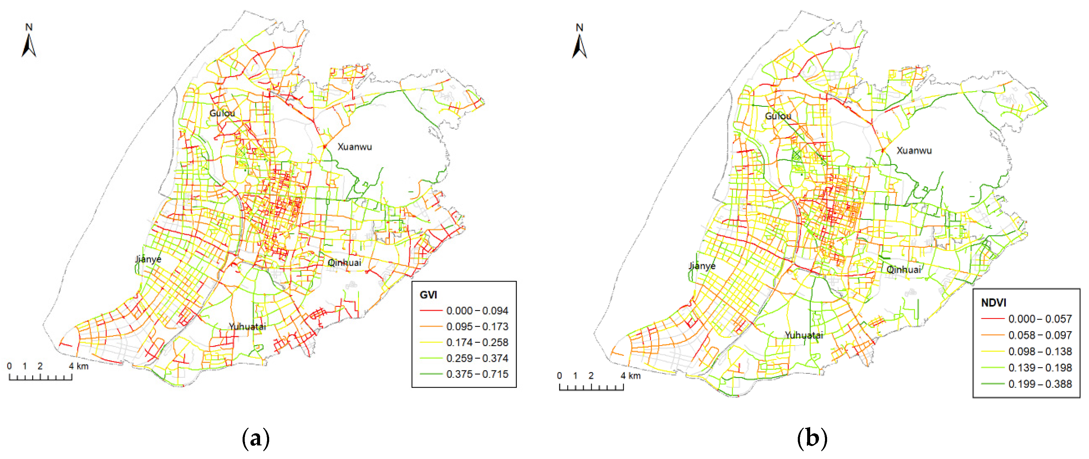
To assess street greenery in multiple aspects, three different indicators were used: the GVI, NDVI and VSD.

The GVI is an indicator that measures the relative quantity of vegetation in the human visual field. The GVI of each point on the street can be calculated by dividing the vegetation pixel count by the total pixel count of the image and then averaging the results from all pictures taken at the site [13] (Equation (1)).

$$GVI=\frac{1}{N}{\sum }_{i=1}^N\frac{T_i+S_i+L_i}{Tota{l}_i}.$$

(1)

$GVI$ indicates the green view index ($0\le GVI\le 1$), and N is the number of images on the site ($1\le N\le 6;$ some sites have less than six pictures). $T_i,S_i\mathrm{and}{L}_i$ are counts of pixels representing trees, shrubs and lawns, respectively, and $Tota{l}_i$ is the pixel count of the whole image.

The NDVI is used to measure greenery from an overhead perspective based on the different wavelengths of the light absorbed by green plant canopies [37]. It can be calculated by Equation (2), where R indicates the red band, and NIR indicates the near-infrared band.

$$NDVI=\frac{NIR-R}{NIR+R}.$$

(2)

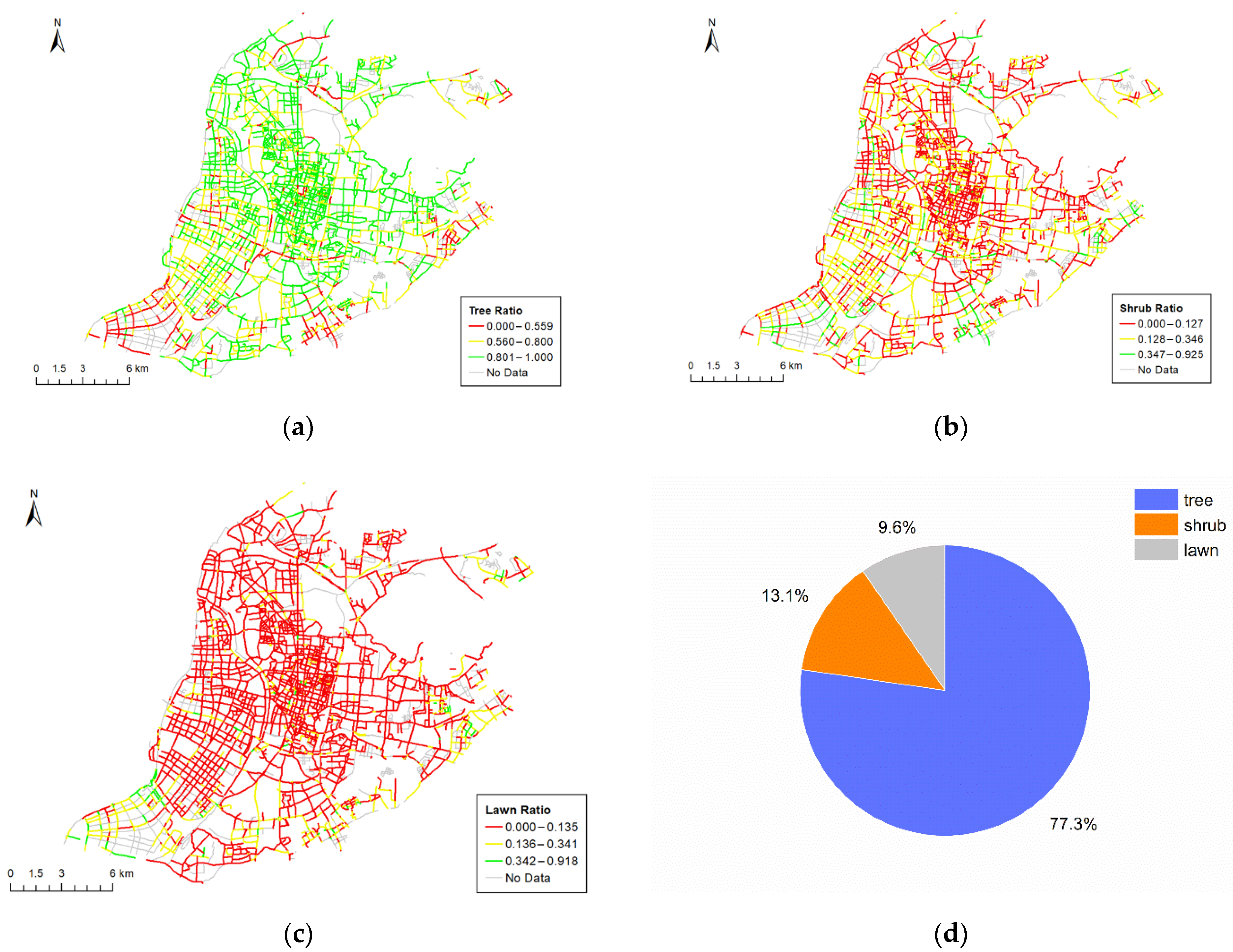
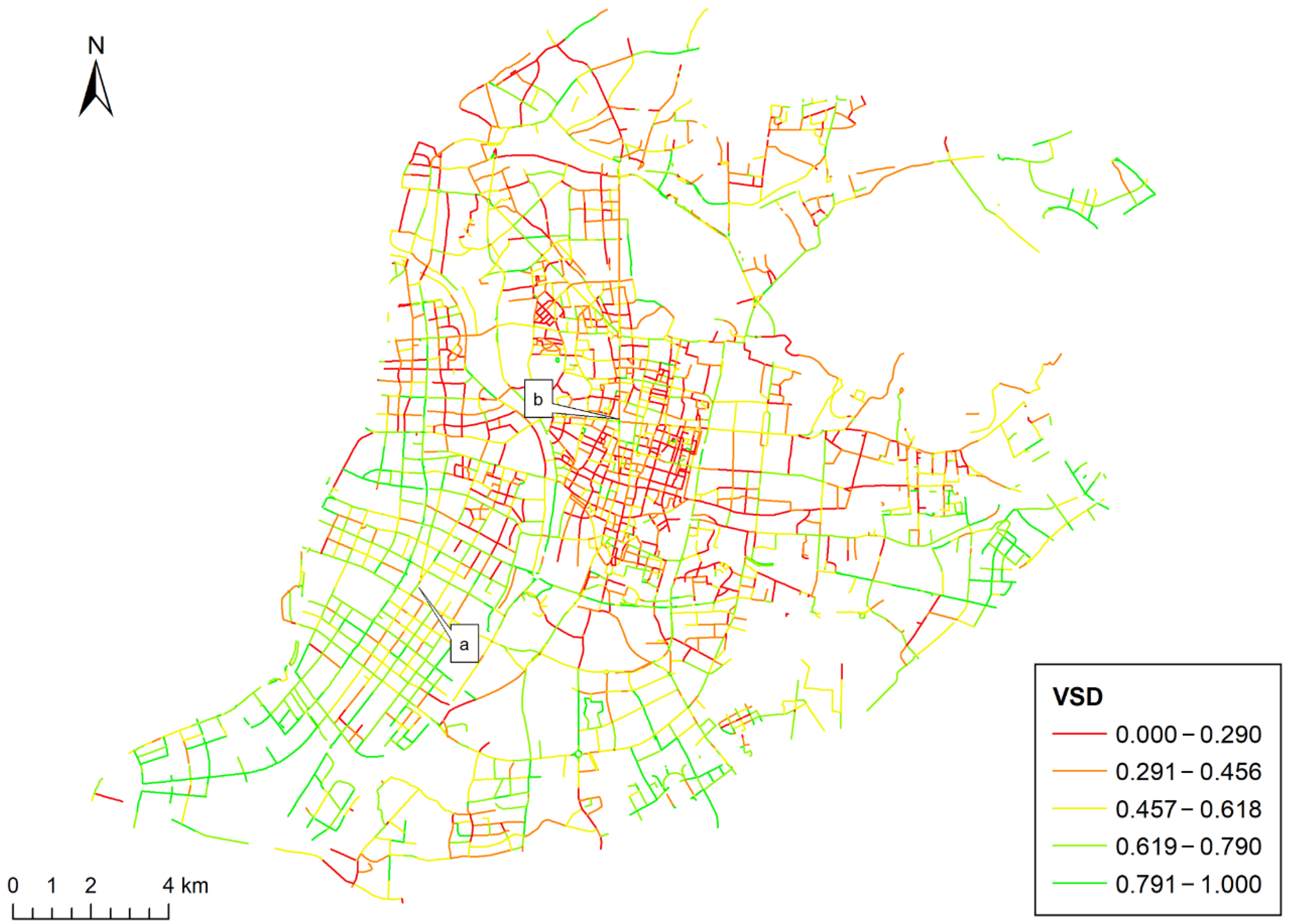
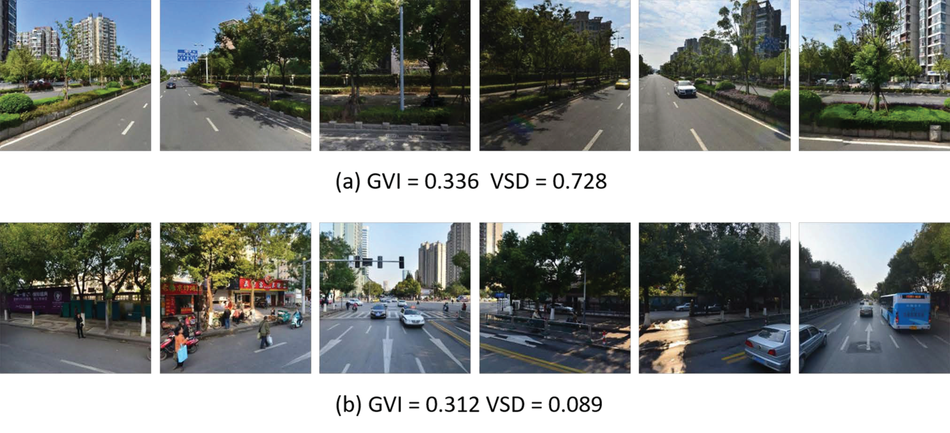
The VSD is an indicator newly proposed in this study based on the Shannon-Wiener index [42]. The Shannon-Wiener index is used initially to evaluate species diversity. In this study, the authors applied the Shannon-Wiener Index to measure the vegetation structure diversity. The equation of VSD can be defined as:

$$VSD=-{\sum }_{i=1}^N{p}_i\ln p_i.$$

(3)

$$p_i=\frac{C_i}{C_{veg}}.$$

(4)

In Equation (3), the range of VSD is (0–1). N could be set at 0, 1, 2 and 3, according to existing vegetation types: trees, shrubs or lawns, and $p_i$ is the proportion of the ith type of vegetation from all vegetation types. A higher VSD indicates greater vegetation structural diversity. In Equation (4), $C_i$ indicates the pixel count of the ith type of vegetation and $C_{veg}$ indicates the pixel counts of all vegetation types.

The street-level GVI result can be obtained by calculating the average GVI of points on each street segment. Considering some street segments have insufficient sample points, the average GVI of these points cannot represent the street-level GVI. Therefore, only street segments satisfying Formula (5) were brought into the greenery assessment, and $\delta$ was set at 80, according to the experiment. L is the road segment’s length, and N is the sample points’ count on the road segment.

$$L/N\le \delta .$$

(5)

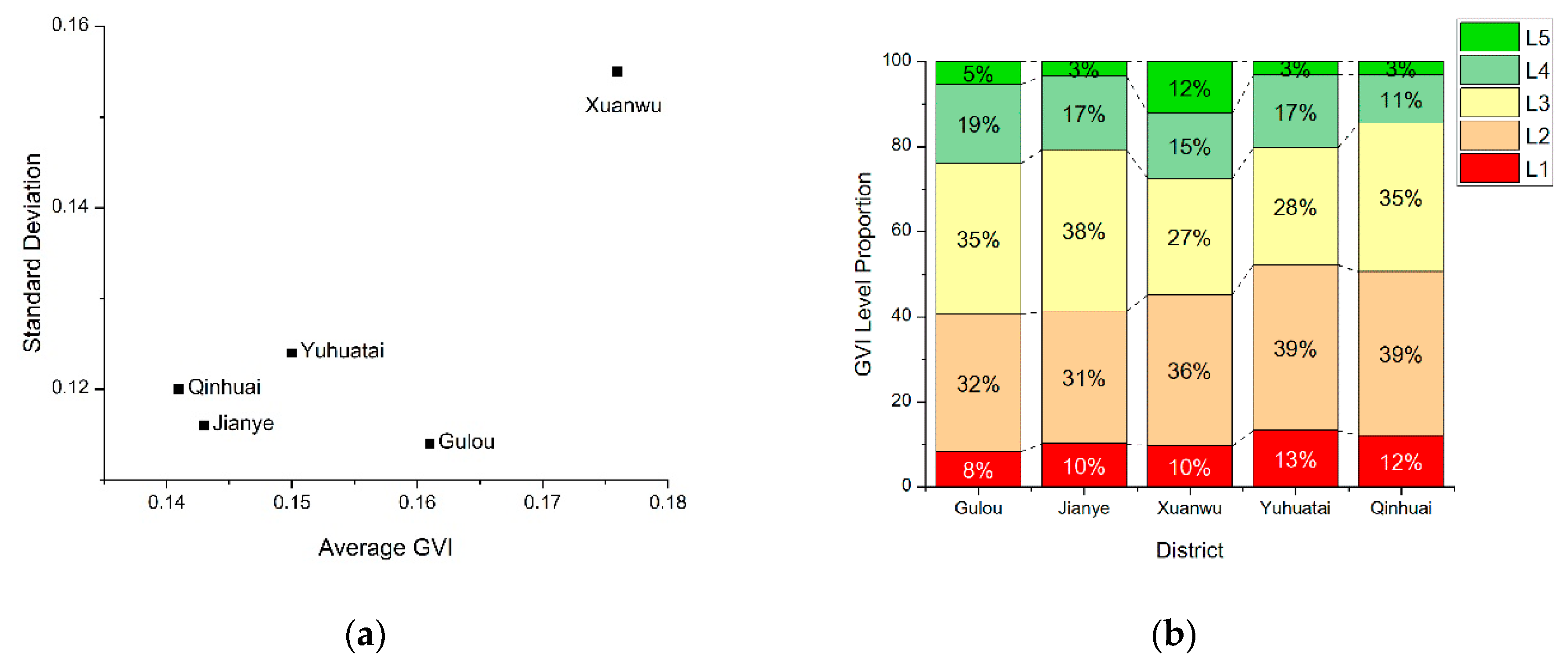
In accordance with Orihara [43], the GVI was classified into 5 levels: L1 (0–0.05), L2 (0.05–0.15), L3 (0.15–0.25), L4 (0.25–0.35) and L5 (0.35–1). Furthermore, the average proportion of vegetation was calculated in this process so the street-level VSD could also be obtained.

To measure the overhead street greenery, the authors used satellite images to calculate the NDVI in the research area and then used the Zonal Statistic tool from ArcGIS software to calculate the street-level NDVI. The Zonal Statistic tool converts road vector data to raster internally, and each road segment is defined as a “zone”. The mean value of NDVI in each zone is calculated, and the result is the street-level NDVI.

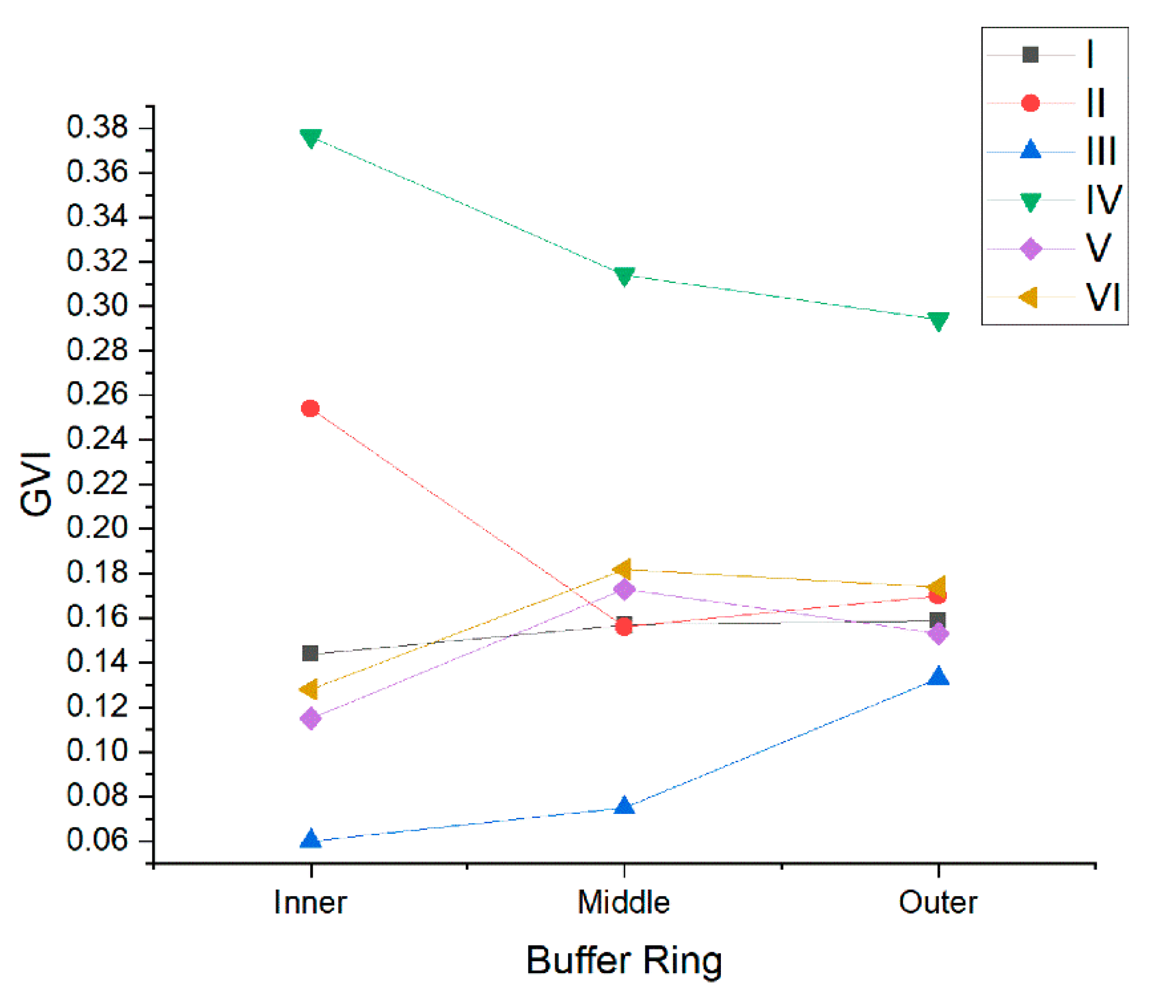
2.5. Hot Spot Analysis and Buffer Analysis on the GVI Results

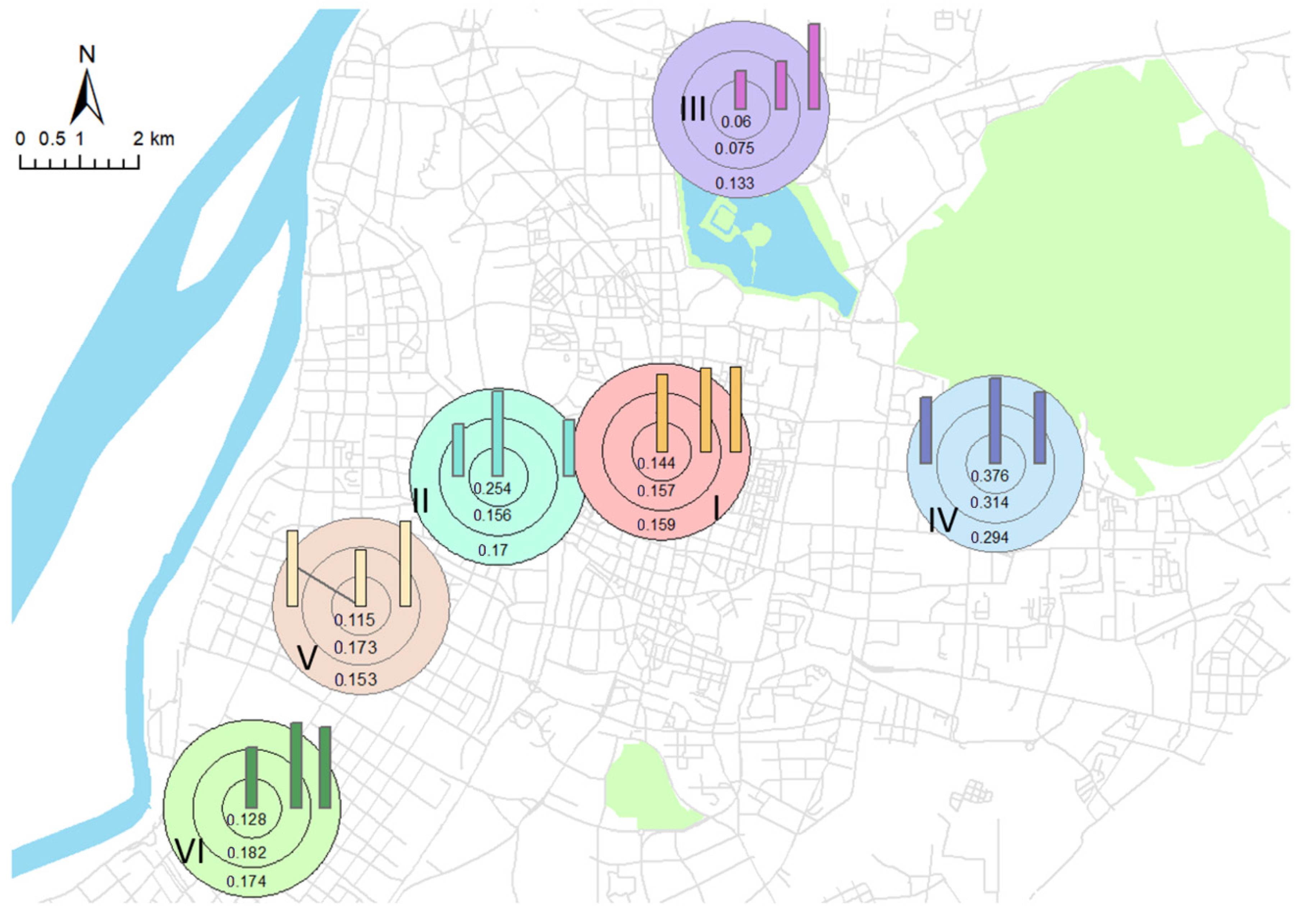
A hot spot analysis is based on Getis-Ord Gi* statistics [44], which identify statistically significant hot spots and cold spots, i.e., spatial clusters of high values and low values. The statistic returns the z-scores and p-scores for the input features. A high z-score and small p-value indicate a hot spot, and a low negative z-score and small p-value indicate cold spots. The calculation is based on Euclidean distance. To analyze the variation trends of the GVI around hot or cold spots, a multi-ring buffer with a 500-m radius was constructed for sample spots, and three rings, named the inner ring, middle ring and outer ring, were created using the “multiple ring buffer” tool in ArcGIS.

3. Results

3.1. Street-Level GVI Distribution in the Urban Area

The results of the street-level GVI distributions show a spatially aggregated characteristic. The higher GVI clusters were A, B and C, and the lower GVI clusters were D, E, F and G. In the inner city with its dense road network, the GVI was found to vary a lot, and the values were mostly lower (Figure 5).

To explore the differences of the GVI distributions in five districts, we calculated the average GVI and standard deviation of each district. The Xuanwu District had the highest average GVI and the highest standard deviation, the Qinhuai District had the lowest average GVI, and the Gulou District had the lowest standard deviation. The GVI rank from high to low was Xuanwu > Gulou > Yuhuatai (northeastern part) > Jianye > Qinhuai. None of the districts had a GVI value of more than 0.25. In addition, the average GVI and standard deviation of Xuanwu District were far higher than those of the other districts (Figure 6a). The proportion of each GVI level is shown in a stacked bar. In the Jianye, Xuanwu and Gulou Districts, streets with a GVI level of L3 or above account for more than half of all streets. For the Xuanwu, Qinhuai and Yuhuatai Districts, L2 accounts for the highest proportion of streets. For the Jianye and Gulou Districts, L3 accounts for the highest proportion of streets. The districts with the highest proportions of L5, L4 and L3 streets are Xuanwu, Gulou and Jianye, respectively (Figure 6b).

Our results show that different districts show different GVI distribution patterns. In Xuanwu District, most of the streets around south of Purple Mountain have a high greenery level (L4 and L5). These streets improve the average GVI of Xuanwu District. However, the streets in other parts of Xuanwu District have a low GVI (L1 andL2), which causes the high standard deviation of the district. In Gulou District, the GVI in the southern part is high (L4 and L5) but that, in the northern part, is low (L1 and L2). The streets on the Qinhuai River banks have high GVI values, which can reach L5 for street greenery. In Jianye District, the GVI in the north is higher than that in the south. L3 and L4 can be reached in the northern part, but only L1 and L2 can be reached in the southern part. In Qinhuai District, only a few streets in the northeastern part near Purple Mountain have high GVI values (L3 and L4). The western part has dense streets, and the GVI is not high (L2 and L3), and the eastern part has a low GVI (L1 and L2). In Yuhuatai District, the GVI of the northern part, which is around a cemetery, is higher (L4 and L5) than that of the southern part (L1 and L2), which is around a railway station (Figure 5).

3.2. GVI Distribution of Different UFZs

The summary statistics of GVI in different UFZs (

Table 4. Summary statistics of the green view index (GVI) in different urban functional zones (UFZs).

Functional Area	Mean (SD)	Min	Max
Commercial Land	0.172 (0.116)	0	0.714
Residential Land	0.193 (0.12)	0	0.796
Industrial Land	0.173 (0.117)	0	0.812
Open Space	0.249 (0.193)	0	0.794
Others	0.218 (0.125)	0	0.678

Open space contains parks, scenic spots, etc.; others contain mainly educational land; SD: standard deviation.

) show that open space has the highest average GVI, followed by others and residential land. The mean GVI value of commercial land and industrial land is relatively low. Besides, the open space has a relatively higher standard deviation than other types of UFZs.

To study the distribution of hot and cold spots in different UFZs, we used a hot spot analysis (Getis-Ord Gi*) to find high and low GVI clusters, shown as hot spots and cold spots (Figure 7), respectively (95% confidence level). The most significant cold spot cluster is located in the inner city, and the largest hot spot cluster is located around Purple Mountain. Hot spots are mainly distributed in open spaces and residential lands, whereas cold spots are mainly located in commercial lands and industrial lands. The spots distributed in others are sparse, but most of them are hot spots. This result is highly consistent with Table 4.

In order to explore the GVI distribution pattern around typical urban areas, six spots, which are located in different UFZs in Nanjing, were selected (

Table 5. Main functions of spots.

Spot	Hot/Cold Spot	Main Function	Location
I	Cold Spot	Commercial Area	Xinjiekou
II	Hot Spot	Park	Mochouhu Park
III	Cold Spot	Railway Station	Nanjing Railway Station
IV	Hot Spot	Scenic Area	Purple Mountain
V	Not Significant	Residential Area	Nanhu
VI	Not Significant	Business Area	Yuantong

). The average GVI of each ring was labeled on each ring, and the bar height reflects the relative magnitude of the GVI value (Figure 8). The GVI variation trend of six spots from the inner ring to the outer ring is displayed in a line chart (Figure 9). Spot IV has the highest GVI and shows a decreasing trend from the inner ring to the outer ring. The streets in the outer ring are closer to the city center, indicating that the street area around Purple Mountain is the high point of the GVI, and the value decreases gradually when closer to the city center. Spot III has the lowest GVI and shows an increasing trend from the inner ring to the outer ring, suggesting that Nanjing Railway Station is a low GVI point in the neighborhood. Spot II has a high GVI in the inner ring but decreases sharply in the middle and outer rings, indicating that the street greenery around the park is adequate, but the “green effect” of the park is only limited to a radius of 1 km. The overall GVI is relatively low in Spot I, but the values from the inner to the outer ring remain stable, suggesting that the overall greenery of commercial areas in the central city require improvement. Spot VII has a relatively low GVI and shows an increasing trend from the inner ring to the middle ring, probably because the areas near point VII represent the densest area of office buildings, which lacks greenery, and the amount of greenery in the outer areas is relatively high because of the existence of residential areas. Spot V has a lower GVI than the middle ring and outer ring, partly due to the location Spot V is on in the intersection of the main road, where the green level is lower than the middle ring, covering more residential area.

3.3. Street-Level NDVI Distribution and Correlations with the GVI

In order to compare the distribution of street-level NDVI and GVI, the levels of two indicators were both classified by the “Jenks Natural Breaks” method, which reduces the variance within classes and maximizes the variance between classes. The overall distribution of the GVI and NDVI is similar, but discrepancies still exist in some areas, especially in the eastern and southern parts of Qinhuai District, the western part of Yuhuatai District, and the northern part of Jianye District (Figure 10).

The correlation analysis between the GVI and NDVI in different administrative districts (

Table 6. Spearman correlations between the GVI and Normalized Difference Vegetation Index (NDVI) in each urban district.

	Qinhuai	Gulou	Jianye	Xuanwu	Yuhuatai
Spearman Coefficient	0.403 **	0.503 **	0.493 **	0.584 **	0.538 **
Sig. (2-tailed)	0.000	0.000	0.000	0.000	0.000
N	5440	4985	4247	3998	2374

** indicates significance at the 0.01 level.

) shows that Xuanwu District has the highest correlation coefficient (0.584), and Qinhuai District has the lowest correlation coefficient (0.403). As for different UFZs, the overall correlation coefficient in the research area is 0.492, which is a moderate correlation. The correlation between the two indicators in different UFZs varies a lot. Open space has the highest correlation coefficient (0.704), and others have the lowest correlation (0.409) (

Table 7. Spearman correlations between the GVI and NDVI in the main city and each UFZ.

	Urban Area	Commercial Land	Residential Land	Industrial Land	Open Space	Others
Spearman Coefficient	0.492 **	0.515 **	0.465 **	0.448 **	0.704 **	0.409 **
Sig. (2-tailed)	0.000	0.000	0.000	0.000	0.000	0.000
N	21,045	4589	10,021	2825	1167	1571

** indicates significance at the 0.01 level.

).

To validate the results in Table 7, we selected the eye-level and overhead views of sample sites in four types of UFZs (Figure 11). Site 1 shows abundant greenery in both perspectives, corresponding to the strong correlation between the GVI and NDVI in open space. Site 2 shows obvious greenery in the eye-level view, whereas greenery in the overhead view is not significant. Site 3 shows plenty of shrubs and lawns in the eye-level view, but trees are sparse. In the overhead view, the shrubs and lawns account for a significant proportion of the image, which corresponds to the lower correlation coefficient in the industrial land. In Site 4, both the eye-level and overhead views of the street greenery are sparse, corresponding to the higher correlation coefficient of commercial land.

3.4. Street Vegetation Composition and VSD Distribution

The proportions and spatial distributions of the three vegetation types vary a lot. Trees are the main element of street vegetation in most of the streets in Nanjing, especially in the central and northern parts of the city, where trees account for more than 80% of the street greenery (Figure 12a). The proportion of shrubs is relatively high in the western and southeastern parts of the city (Figure 12b). Most of the streets have a relatively small proportion of lawns; the proportion of lawns is relatively high only in the southwestern and eastern parts of the city (Figure 12c). For the whole area, trees account for more than 77% of the street greenery, followed by shrubs (13.1%) and lawns (9.6%) (Figure 12d).

Based on the proportions of the three vegetation types, we further explored the distribution of VSD. The areas with high VSD were mainly located in southern parts of the city, especially in the new city. The VSD in the central and northern parts, which mainly belong to the old city, is relatively low (Figure 13). This distribution pattern does not seem consistent with that of the GVI (Figure 5). Through the Spearman correlation analysis of the GVI and VSD in the urban area, there was a significant weak negative correlation between them ($r_{Spearman}=-{0.256}^{**}$, Sig. (2-tailed) = 0.000). According to the example of the street view pictures (Figure 14) on point a and b in Figure 13, the GVI values of the two points are close, but VSD has large differences. Point a achieved a good combination of trees and shrubs, whereas point b has only trees and lacks lower greenery.

3.5. The GVI and VSD of Different Road Levels

Box plots were used to represent the GVI of different road levels in the research area (Figure 15a). The lines across the boxes represent the medians, and the squares in the boxes represent the means, whereas the bottoms and tops of the boxes show the locations of the first (Q1) and third quartiles (Q3). The ends of the whiskers represent one and a half times the interquartile range (1.5QR) and the black circles represent the outliers. The expressway has the lowest average GVI and most concentrated GVI distribution, whereas the other three road levels have similar average values. The main road and branch road show a larger variation in values, whereas the GVI distribution of the secondary road is relatively concentrated.

As for VSD, the expressway has the highest average value, whereas the branch road obtains the lowest value. The main road and the secondary road have similar average values. The VSD of the expressway has a high level of agreement with each other, whereas the GVI values in the secondary road and branch road have large discrepancies (Figure 15b). We selected the TSV images of typical sites on each level of the road to validate the results (Figure 16). According to our manual audits on TSV images in different areas of the study area, the expressways are usually set up with a combination of trees and shrubs, while the branch roads are often planted with single trees without lower vegetation, like the last picture in Figure 16.

The mean GVI and VSD values of different road levels in the old city and new city were calculated, respectively (

Table 8. Mean GVI/VSD of different road levels in the main city, the old city and new city.

City Area	Expressway	Main Road	Secondary Road	Branch Road
Old city (GVI)	0.141	0.212	0.186	0.152
New city (GVI)	0.134	0.144	0.192	0.196
Old city (VSD)	0.636	0.474	0.419	0.376
New city (VSD)	0.701	0.709	0.631	0.536

). Both areas have a low level of GVI on expressways and a medium level of GVI on secondary roads. However, large differences exist on the main roads and branch roads between the old city and the new city. The old city has a higher GVI level than the new city on the main road, whereas the new city has a higher GVI level than the old city on the branch road. In addition, the GVI of main roads is higher than that of branch roads in the old city, while the new city presents an opposite trend. Compared with GVI, the trend of VSD in the old city and the new city is relatively consistent. The VSD in the new city is entirely higher than that in the old city, and the VSD declines with the decrease of road level in both the old city and new city, except for the expressway and main road in the new city.

4. Discussion

This study used three indicators: the GVI, NDVI, and VSD to assess the street greenery with street views and satellite images. Compared with research using a single assessment indicator, this study compared overhead greenery and eye-level greenery based on different UFZs. We imported a new indicator VSD, which is essential for maintaining diversified greening landscapes, which is more comprehensive and objective for a street greenery assessment.

4.1. Summary and Practical Implications of GVI Evaluation Results

The GVI distribution in the urban area of Nanjing showed an aggregating pattern. Low-value points are concentrated in the city center (old city), whereas high-value points are concentrated in the old city’s periphery. The distributions of GVI in Beijing [27,36,45], Hong Kong [17] and Boston [46] are similar to this, but in the Pearl River Delta cities [47] Shanghai [36,48] and Singapore [29], the pattern is that the GVI is high in the city center and low in its periphery, suggesting that the distribution of the GVI may be related to the specific road network structure. Taking Pearl River Delta City as an example, the narrow roads in the central urban area and the long ages of street trees lead to higher GVI [47]. However, in cities like Beijing, the branch roads in the city center, i.e., Hutongs [49], have a long history and lack of renewal, which is similar to the conditions of branch roads of Nanjing City. It is noteworthy that the hot spots in Nanjing are scattered around mountains, parks and waters, such as Purple Mountain, Qinhuai River, Yuhuatai Martyrs Memorial Park and Mochouhu Park. The results confirm that street greenery’s distribution pattern in the Nanjing urban area is significantly affected by natural elements such as mountains and waters.

Branch roads in the old city have low levels of street greenery (Table 8). This may be due to the limited space for planting trees on these roads. However, improving the greenery levels of these roads is essential. Low-class roads provide high walkability, safety and close contact with green plants, which is preferred by residents walking or cycling on these roads. Well greenery on low-class roads can encourage residents to do more activities [49]. Furthermore, the old city has a higher proportion of older adults than in the new city (

Table 9. Distributions of the elderly populations in each district [51].

District	District Type	Older Adults Number	Older Adults Proportion
Xuanwu	Old City	81,420	12.5%
Gulou	Old City	177,394	14.0%
Qinhuai	Old City	175,710	14.0%
Jianye	New City	50,004	11.7%
Yuhuatai	New City	44,549	11.4%

). A high level of greenery can promote physical activity engagement by older adults [7], which is beneficial to their health [50]. Considering the limited spaces of branch roads, vertical forms of greenery, such as creepers or box planting, may be suitable for greenery improvements in these high-density urban areas.

4.2. The Functions and Relationships of the GVI, NDVI and VSD

The three indicators reflect different aspects of street greenery. The GVI is used to measure the amount of greenery perceived by pedestrians, the NDVI measures the green coverage from an overhead view and VSD presents the diversity of different vegetation levels.

The overall correlation between the GVI and NDVI is moderate, suggesting that the GVI and NDVI show different perspectives of street greenery. The results are similar to the findings of Helbich [37] and Ye [29], which also report weak (0.225) or moderate (0.606) correlations between the two indicators. However, there are variations of the correlations in different UFZ types. In open spaces like parks and scenic spots, the perceived greenery is abundant both in the eye-level and overhead views. Therefore, the greenery assessment results in open spaces is relatively consistent. This conclusion is not consistent with Lu [17], which suggested that the GVI is much lower than the NDVI in country parks or other preserved areas. The discrepancy originated from a different research scale. Lu compared the two indicators at a regional level, which is different from the street-level comparison in this study. The NDVI calculation at the regional level will include plenty of vegetation far away from the road, while the calculation of the GVI is still limited to the street space. With the buffer distances increasing from the street, the correlation coefficients between the GVI and green vegetation coverage decrease [28], reflecting the necessity of unifying the calculation scale to the street level. As for the residential land and industrial land, the correlations of the two indicators are both weak. Vertical greenery is more than horizontal greenery in residential lands, while it is the opposite in industrial lands (Figure 11). In commercial lands, both the eye-level and overhead views of street greenery are low, leading to a relatively high correlation between the two indicators. This result supports the findings of Lu [17] and Ye [29].

The distribution of VSD presents a tendency that the values in the old city are lower than those in the new city. The roads in the old city are usually dominated by trees, while the roads in the new city are arranged with multi-level vegetation, usually with tree–shrub structures or tree–shrub–herb structures (Figure 14), so the VSD will be significantly different. The comparisons between Figure 5 and Figure 13 show that the distributions of the GVI and VSD are not consistent, and the two indicators present a weak negative correlation. Only in the middle and north of Jianye District can the two indicators achieve a favorable balance. This phenomenon suggests a mismatch between the amount of greenery and structural diversity in the street of Nanjing. For the old city, especially the branch roads (Figure 16), it is necessary to strengthen the lower greenery, such as shrubs and herbs; for the new urban area, it is necessary to increase tree planting to enhance the perceived greenery.

It is highly recommended that multiple indicators be taken into account in the evaluation of street greenery. For example, according to the needs of street greenery construction, three indicators can be given different weights to calculate a comprehensive greening quality score conducive to the construction of greener and multi-level street greening infrastructures. Furthermore, the statistical results based on different UFZs and road types can give urban planners references to optimize the greenery of different areas and roads.

4.3. Limitations and Future Works

There are also some limitations in our study. Firstly, the street view images were taken in 2014 and are maybe out-of-date for some areas, especially in Jianye District, which is under construction and has apparent yearly variations in the urban scene. Additionally, vegetation growth and succession is also a non-negligible factor. These mismatches of time may cause the greenery value collected to be lower than the current value. Secondly, the diversity of tree species was not considered with the limitation of categories in the training data, and this is also an essential measurement of street greenery. Planting different kinds of trees can improve the level of happiness and the visual perception of pedestrians. In future works, some explorations of street greenery could be made. First, the street view images were taken by cameras on cars and may be different from what pedestrians see on wide roads with divisions of the vehicle and pedestrian lanes. Thus, quantitative relationships between greenery from a vehicle perspective and from a pedestrian perspective can be established, and predictions can be made of the pedestrians’ visual greenery by the GVI calculated by street view images, which can represent the pedestrians’ perceptions of vegetation more accurately. Secondly, variation detection is an important research topic in the remote-sensing area, but in the urban street view perception area, related work is rare because of the street view API limitation. If continuing years of street view data can be found, temporal variations of street greenery can be analyzed, and the greenery in the future may be predicted according to a time sequence. Thirdly, Virtual Reality (VR)-based 3D data representation could be introduced to the eye-level greenery evaluation with a higher sense of immersion and a more detailed depiction of the street scene [52,53].

5. Conclusions

This study used multiple indicators to assess the street greenery in the urban areas of Nanjing from different perspectives. The results presented the discrepancies of eye-level greenery and its relationships with overhead greenery in different functional areas. Moreover, the study analyzed the distribution of vegetation compositions and compared the distribution of eye-level greenery with vegetation structural diversity in different road levels. As for different urban areas, the greening amount of the old city is more substantial than that of the new city, but the greening structure is not as rich as that of the old city. The results indicated that using different indicators to evaluate the street greenery will produce diverse results for different urban areas, which is more comprehensive and objective than using a single index and has a more decisive guiding significance for further improvement of the quality of urban greening.

References

1. Samara, T.; Tsitsoni, T. The effects of vegetation on reducing traffic noise from a city ring road. Noise Control Eng. J. 2011, 59, 68–74. [Google Scholar] [CrossRef]
2. Ferrini, F.; Fini, A.; Mori, J.; Gori, A.J.S. Role of Vegetation as a Mitigating Factor in the Urban Context. Sustainability 2020, 12, 4247. [Google Scholar] [CrossRef]
3. Shishegar, N. The impact of green areas on mitigating urban heat island effect: A review. Int. J. Environ. Sustain. 2014, 9, 119–130. [Google Scholar] [CrossRef]
4. Zhang, B.; Xie, G.-D.; Gao, J.-X.; Yang, Y. The cooling effect of urban green spaces as a contribution to energy-saving and emission-reduction: A case study in Beijing, China. Build. Environ. 2014, 76, 37–43. [Google Scholar] [CrossRef]
5. Jim, C.Y.; Chen, W.Y. Assessing the ecosystem service of air pollutant removal by urban trees in Guangzhou (China). J. Environ. Manag. 2008, 88, 665–676. [Google Scholar] [CrossRef]
6. Lu, Y. Using Google Street View to investigate the association between street greenery and physical activity. Landsc. Urban. Plan. 2019, 191, 103435. [Google Scholar] [CrossRef]
7. Yang, Y.; He, D.; Gou, Z.; Wang, R.; Liu, Y.; Lu, Y. Association between street greenery and walking behavior in older adults in Hong Kong. Sustain. Cities Soc. 2019, 51. [Google Scholar] [CrossRef]
8. Li, X.; Ghosh, D. Associations between Body Mass Index and Urban “Green” Streetscape in Cleveland, Ohio, USA. Int. J. Environ. Res. Public Health 2018, 15, 2186. [Google Scholar] [CrossRef] [Green Version]
9. Wang, R.; Helbich, M.; Yao, Y.; Zhang, J.; Liu, P.; Yuan, Y.; Liu, Y. Urban greenery and mental wellbeing in adults: Cross-sectional mediation analyses on multiple pathways across different greenery measures. Environ. Res. 2019, 176, 108535. [Google Scholar] [CrossRef] [Green Version]
10. Liu, Y.; Wang, R.; Xiao, Y.; Huang, B.; Chen, H.; Li, Z. Exploring the linkage between greenness exposure and depression among Chinese people: Mediating roles of physical activity, stress and social cohesion and moderating role of urbanicity. Health Place 2019, 58, 102168. [Google Scholar] [CrossRef]
11. Li, X.; Zhang, C.; Li, W.; Kuzovkina, Y.A.; Weiner, D. Who lives in greener neighborhoods? The distribution of street greenery and its association with residents’ socioeconomic conditions in Hartford, Connecticut, USA. Urban. For. Urban. Green. 2015, 14, 751–759. [Google Scholar] [CrossRef]
12. Troy, A.; Morgan Grove, J.; O’Neil-Dunne, J. The relationship between tree canopy and crime rates across an urban–rural gradient in the greater Baltimore region. Landsc. Urban. Plan. 2012, 106, 262–270. [Google Scholar] [CrossRef]
13. Yang, J.; Zhao, L.; McBride, J.; Gong, P. Can you see green? Assessing the visibility of urban forests in cities. Landsc. Urban. Plan. 2009, 91, 97–104. [Google Scholar] [CrossRef]
14. Aoki, Y. Relationship between percieved greenery and width of visual fields. J. Jpn. Inst. Landsc. Archit. 1987, 51, 1–10. [Google Scholar] [CrossRef]
15. Long, Y.; Liu, L. How green are the streets? An analysis for central areas of Chinese cities using Tencent Street View. PLoS ONE 2017, 12, e0171110. [Google Scholar] [CrossRef] [PubMed] [Green Version]
16. Villeneuve, P.J.; Ysseldyk, R.L.; Root, A.; Ambrose, S.; Dimuzio, J.; Kumar, N.; Shehata, M.; Xi, M.; Seed, E.; Li, X.; et al. Comparing the normalized difference vegetation index with the google street view measure of vegetation to assess associations between greenness, walkability, recreational physical activity, and health in Ottawa, Canada. Int. J. Environ. Res. Public Health 2018, 15, 1719. [Google Scholar] [CrossRef] [Green Version]
17. Lu, Y.; Yang, Y.; Sun, G.; Gou, Z. Associations between overhead-view and eye-level urban greenness and cycling behaviors. Cities 2019, 88, 10–18. [Google Scholar] [CrossRef]
18. Chen, X.; Meng, Q.; Hu, D.; Zhang, L.; Yang, J. Evaluating greenery around streets using baidu panoramic street view images and the panoramic green view index. Forests 2019, 10, 1109. [Google Scholar] [CrossRef] [Green Version]
19. Gong, F.Y.; Zeng, Z.C.; Zhang, F.; Li, X.; Ng, E.; Norford, L.K. Mapping sky, tree, and building view factors of street canyons in a high-density urban environment. Build. Environ. 2018, 134, 155–167. [Google Scholar] [CrossRef]
20. Li, X.; Zhang, C.; Li, W.; Ricard, R.; Meng, Q.; Zhang, W. Assessing street-level urban greenery using Google Street View and a modified green view index. Urban. For. Urban. Green. 2015, 14, 675–685. [Google Scholar] [CrossRef]
21. Liu, L.; Silva, E.A.; Wu, C.; Wang, H. A machine learning-based method for the large-scale evaluation of the qualities of the urban environment. Comput. Environ. Urban. Syst. 2017, 65, 113–125. [Google Scholar] [CrossRef]
22. Zhang, L.; Ye, Y.; Zeng, W.; Chiaradia, A. A systematic measurement of street quality through multi-sourced Urban data: A human-oriented analysis. Int. J. Environ. Res. Public Health 2019, 16, 1782. [Google Scholar] [CrossRef] [PubMed] [Green Version]
23. Zhang, F.; Zhou, B.; Liu, L.; Liu, Y.; Fung, H.H.; Lin, H.; Ratti, C. Measuring human perceptions of a large-scale urban region using machine learning. Landsc. Urban. Plan. 2018, 180, 148–160. [Google Scholar] [CrossRef]
24. Yin, L.; Wang, Z. Measuring visual enclosure for street walkability: Using machine learning algorithms and Google Street View imagery. Appl. Geogr. 2016, 76, 147–153. [Google Scholar] [CrossRef]
25. Blecic, I.; Cecchini, A.; Trunfio, G.A. Towards Automatic Assessment of Perceived Walkability. In Computational Science and Its Applications—ICCSA 2018, Pt Iii; Gervasi, O., Murgante, B., Misra, S., Stankova, E., Torre, C.M., Rocha, A., Taniar, D., Apduhan, B.O., Tarantino, E., Ryu, Y., Eds.; Springer: Cham, Switzerland, 2018; Volume 10962, pp. 351–365. [Google Scholar]
26. Yu, S.; Yu, B.; Song, W.; Wu, B.; Zhou, J.; Huang, Y.; Wu, J.; Zhao, F.; Mao, W. View-based greenery: A three-dimensional assessment of city buildings’ green visibility using Floor Green View Index. Landsc. Urban. Plan. 2016, 152, 13–26. [Google Scholar] [CrossRef]
27. Dong, R.C.; Zhang, Y.L.; Zhao, J.Z. How Green Are the Streets within the Sixth Ring Road of Beijing? An Analysis Based on Tencent Street View Pictures and the Green View Index. Int. J. Environ. Res. Public Health 2018, 15, 1367. [Google Scholar] [CrossRef] [Green Version]
28. Yu, X.; Zhao, G.; Chang, C.; Yuan, X.; Heng, F. BGVI: A new index to estimate street-side greenery using Baidu Street View Image. Forests 2019, 10, 3. [Google Scholar] [CrossRef] [Green Version]
29. Ye, Y.; Richards, D.; Lu, Y.; Song, X.; Zhuang, Y.; Zeng, W.; Zhong, T. Measuring daily accessed street greenery: A human-scale approach for informing better urban planning practices. Landsc. Urban. Plan. 2019, 191. [Google Scholar] [CrossRef]
30. Antos, J.A. Understory Plants in Temperate Forests. In Forests and Forests Plants; John, N., Owens, H.G.L., Eds.; Encyclopedia of Life Support Systems (EOLSS), Developed under the Auspices of the UNESCO; Eolss Publishers: Paris, France, 2009; Volume I, pp. 262–279. [Google Scholar]
31. Threlfall, C.G.; Mata, L.; Mackie, J.A.; Hahs, A.K.; Stork, N.E.; Williams, N.S.G.; Livesley, S.J. Increasing biodiversity in urban green spaces through simple vegetation interventions. J. Appl. Ecol. 2017, 54, 1874–1883. [Google Scholar] [CrossRef] [Green Version]
32. Nicholls, F. The value of understorey vegetation. In Land for Wildlife Notes; Department of Natural Resources and Environment: State of Victoria, Australia, 2000; pp. 1–3. [Google Scholar]
33. Saumel, I.; Weber, F.; Kowarik, I. Toward livable and healthy urban streets: Roadside vegetation provides ecosystem services where people live and move. Environ. Sci. Policy 2016, 62, 24–33. [Google Scholar] [CrossRef]
34. Harris, V.; Kendal, D.; Hahs, A.K.; Threlfall, C.G. Green space context and vegetation complexity shape people’s preferences for urban public parks and residential gardens. Landsc. Res. 2018, 43, 150–162. [Google Scholar] [CrossRef]
35. Drillet, Z.; Fung, T.K.; Leong, R.A.T.; Sachidhanandam, U.; Edwards, P.; Richards, D. Urban Vegetation Types are Not Perceived Equally in Providing Ecosystem Services and Disservices. Sustainability 2020, 12, 2076. [Google Scholar] [CrossRef] [Green Version]
36. Fu, X.; Jia, T.; Zhang, X.; Li, S.; Zhang, Y. Do street-level scene perceptions affect housing prices in Chinese megacities? An analysis using open access datasets and deep learning. PLoS ONE 2019, 14. [Google Scholar] [CrossRef] [PubMed]
37. Helbich, M.; Yao, Y.; Liu, Y.; Zhang, J.; Liu, P.; Wang, R. Using deep learning to examine street view green and blue spaces and their associations with geriatric depression in Beijing, China. Environ. Int. 2019, 126, 107–117. [Google Scholar] [CrossRef] [PubMed]
38. Cheng, L.; Chu, S.; Zong, W.; Li, S.; Wu, J.; Li, M. Use of Tencent Street View imagery for visual perception of streets. ISPRS Int. J. Geo-Inf. 2017, 6, 265. [Google Scholar] [CrossRef]
39. Ge, P.P.; He, J.; Zhang, S.H.; Zhang, L.W.; She, J.F. An Integrated Framework Combining Multiple Human Activity Features for Land Use Classification. ISPRS Int. J. Geo-Inf. 2019, 8, 16. [Google Scholar] [CrossRef] [Green Version]
40. Zhao, H.; Shi, J.; Qi, X.; Wang, X.; Jia, J. Pyramid Scene Parsing Network. In Proceedings of the 2017 IEEE Conference on Computer Vision and Pattern Recognition (CVPR), Honolulu, HI, USA, 21–26 July 2017; pp. 6230–6239. [Google Scholar]
41. Zhou, B.; Zhao, H.; Puig, X.; Xiao, T.; Fidler, S.; Barriuso, A.; Torralba, A. Semantic Understanding of Scenes Through the ADE20K Dataset. Int. J. Comput. Vis. 2019, 127, 302–321. [Google Scholar] [CrossRef] [Green Version]
42. Spellerberg, I.F.; Fedor, P.J. A tribute to Claude Shannon (1916–2001) and a plea for more rigorous use of species richness, species diversity and the ‘Shannon–Wiener’ Index. Glob. Ecol. Biogeogr. 2003, 12, 177–179. [Google Scholar] [CrossRef] [Green Version]
43. Orihara, N. A study of economic valuation for the landscape—An empirical analysis of the effects of landscape on real-estate values. Seas. Res. Rep. UR 2006, 2006, 4–13. [Google Scholar]
44. Getis, A.; Ord, J.K. The analysis of spatial association by use of distance statistics. In Perspectives on Spatial Data Analysis; Springer: Berlin/Heidelberg, Germany, 2010; pp. 127–145. [Google Scholar]
45. Zhang, Y.; Dong, R. Impacts of street-visible greenery on housing prices: Evidence from a hedonic price model and a massive street view image dataset in Beijing. ISPRS Int. J. Geo-Inf. 2018, 7, 104. [Google Scholar] [CrossRef] [Green Version]
46. Li, X.; Santi, P.; Courtney, T.K.; Verma, S.K.; Ratti, C. Investigating the association between streetscapes and human walking activities using Google Street View and human trajectory data. Trans. GIS 2018, 22, 1029–1044. [Google Scholar] [CrossRef]
47. Chen, J.; Zhou, C.; Li, F.J.E.I. Quantifying the green view indicator for assessing urban greening quality: An analysis based on Internet-crawling street view data. Ecol. Indic. 2020, 113, 106192. [Google Scholar] [CrossRef]
48. Ye, Y.; Xie, H.; Fang, J.; Jiang, H.; Wang, D. Daily Accessed Street Greenery and Housing Price: Measuring Economic Performance of Human-Scale Streetscapes via New Urban Data. Sustainability 2019, 11, 1741. [Google Scholar] [CrossRef] [Green Version]
49. Wu, J.; Wang, B.; Ta, N.; Zhou, K.; Chai, Y.J.U.F.; Greening, U. Does street greenery always promote active travel? Evidence from Beijing. Urban For. Urban Green. 2020, 56, 126886. [Google Scholar] [CrossRef]
50. Pahor, M.; Guralnik, J.M.; Ambrosius, W.T.; Blair, S.; Bonds, D.E.; Church, T.S.; Espeland, M.A.; Fielding, R.A.; Gill, T.M.; Groessl, E.J.; et al. Effect of Structured Physical Activity on Prevention of Major Mobility Disability in Older Adults: The LIFE Study Randomized Clinical Trial. JAMA 2014, 311, 2387–2396. [Google Scholar] [CrossRef] [PubMed]
51. Population Census Office under the State Council (PCO). Tabulation on the 2010 Population Census of the People’s Republic of China by County; China Statistics Press: Beijing, China, 2012.
52. Edler, D.; Keil, J.; Wiedenlübbert, T.; Sossna, M.; Kühne, O.; Dickmann, F.; Information, G. Immersive VR experience of redeveloped post-industrial sites: The example of “Zeche Holland” in Bochum-Wattenscheid. KN-J. Cartogr. Geogr. Inf. 2019, 69, 267–284. [Google Scholar] [CrossRef] [Green Version]
53. Hruby, F.; Castellanos, I.; Ressl, R. Cartographic Scale in Immersive Virtual Environments. KN-J. Cartogr. Geogr. Inf. 2020, 1–7. [Google Scholar] [CrossRef]
Figure 1. Location of the study area. The urban area of Nanjing consists of Gulou, Xuanwu, Jianye, Qinhuai, and the northeastern Yuhuatai district. Xinjiekou is the largest commercial area located in the city center. The inner city includes the area inside the inner ring road, also called the “old city” of Nanjing. The new city is a newly built district named “Hexi New City”.
Forests 11 01347 g001
Figure 2. Four types of topological errors exist in OpenStreetMap (OSM) road networks. The red symbol in the first row shows the location of existing errors, and the second row shows the results of the topological correction.
Forests 11 01347 g002
Figure 3. Acquiring street view images in six directions. (a) Original street view images from six directions. (b) Segmentation results of street view images.
Forests 11 01347 g003
Figure 4. Image semantic segmentation result of a sample image. (a) The original street view picture. (b) The segmentation result by the Pyramid Scene Parsing Network (PSPNet) and corresponding categories.
Forests 11 01347 g004
Figure 5. Street–level distributions of the green view index (GVI) in Nanjing. The higher GVI clusters were A, B and C, and the lower GVI clusters were D, E, F and G. In the inner city with its dense road network, the GVI was found to vary a lot, and the values were mostly lower.
Forests 11 01347 g005
Figure 6. District distribution of street greenery. (a) Average and standard deviation of the GVI in each district. (b) Proportions of the 5 GVI levels in the 5 districts. The levels include L1 (0–0.05), L2 (0.05–0.15), L3 (0.15–0.25), L4 (0.25–0.35) and L5 (0.35–1).
Forests 11 01347 g006
Figure 7. Hot spot analysis map overlaid on the urban functional zone (UFZ) map.
Forests 11 01347 g007
Figure 8. GVI distribution pattern around six typical spots in the Nanjing urban area. I, II, III, IV, V and VI represent the commercial area, park, railway station, scenic area, high-density residential area and business area. Three-ring buffers were constructed every 500 m from each spot, and the average GVI values are labeled on the rings and shown by the bars.
Forests 11 01347 g008
Figure 9. GVI variation trend from the inner ring to the outer ring in 6 spots (I–VII). The horizontal axis represents three buffer rings. The vertical axis represents the average GVI in each ring.
Forests 11 01347 g009
Figure 10. Comparison of the street–level GVI and Normalized Difference Vegetation Index (NDVI). Levels were both classified by the natural break method. (a) Street–level GVI distribution. (b) Street–level NDVI distribution.
Forests 11 01347 g010
Figure 11. Comparison of street greenery from the eye-level and overhead perspective in different urban functional zones (UFZs). The eye-level image came from the street view image, and the overhead view came from Google Maps. The red marker in each satellite image indicates the location of the street view image.
Forests 11 01347 g011
Figure 12. Vegetation compositions of the research area. Levels were classified by the natural break method. (a) The proportion of trees. (b) The proportion of shrubs. (c) The proportion of lawns. (d) Proportions of the three vegetation types.
Forests 11 01347 g012
Figure 13. Street–level vegetation structural diversity (VSD) distribution. Levels were classified by the natural break method.
Forests 11 01347 g013
Figure 14. Examples of roads with different levels of VSD. (a) Street with high VSD in the southern part of the city. Trees and shrubs are combined in layers. (b) Street with low VSD in the city center. Trees are the only vegetation.
Forests 11 01347 g014
Figure 15. GVI and VSD distributions of different road levels in box plots. (a) Box plots of GVI distribution. (b) Box plots of VSD distribution.
Forests 11 01347 g015
Figure 16. Sample street view images of different road levels, and the VSD values are labeled below the pictures.
Forests 11 01347 g016