Article

Mapping Tree Species Deciduousness of Tropical Dry Forests Combining Reflectance, Spectral Unmixing, and Texture Data from High-Resolution Imagery

by
Astrid Helena Huechacona-Ruiz
1,
Juan Manuel Dupuy
1,
Naomi B. Schwartz
2,
Jennifer S. Powers
3,
Casandra Reyes-García
1,
Fernando Tun-Dzul
1 and
José Luis Hernández-Stefanoni
1,*
1
Centro de Investigación Científica de Yucatán A.C., Unidad de Recursos Naturales, Calle 43 # 130, x 32 y 34 Colonia Chuburná de Hidalgo, Mérida CP 97205, Yucatán, Mexico
2
Department of Geography, University of British Columbia, Vancouver, BC V6T 1Z2, Canada
3
Department of Ecology, Evolution and Behavior, University of Minnesota, Saint Paul, MN 55108, USA
*
Author to whom correspondence should be addressed.
Forests 2020, 11(11), 1234; https://doi.org/10.3390/f11111234
Submission received: 8 October 2020 / Revised: 14 November 2020 / Accepted: 19 November 2020 / Published: 23 November 2020
(This article belongs to the Section Forest Inventory, Modeling and Remote Sensing)

Abstract

:
In tropical dry forests, deciduousness (i.e., leaf shedding during the dry season) is an important adaptation of plants to cope with water limitation, which helps trees adjust to seasonal drought. Deciduousness is also a critical factor determining the timing and duration of carbon fixation rates, and affecting energy, water, and carbon balance. Therefore, quantifying deciduousness is vital to understand important ecosystem processes in tropical dry forests. The aim of this study was to map tree species deciduousness in three types of tropical dry forests along a precipitation gradient in the Yucatan Peninsula using Sentinel-2 imagery. We propose an approach that combines reflectance of visible and near-infrared bands, normalized difference vegetation index (NDVI), spectral unmixing deciduous fraction, and several texture metrics to estimate the spatial distribution of tree species deciduousness. Deciduousness in the study area was highly variable and decreased along the precipitation gradient, while the spatial variation in deciduousness among sites followed an inverse pattern, ranging from 91.5 to 43.3% and from 3.4 to 9.4% respectively from the northwest to the southeast of the peninsula. Most of the variation in deciduousness was predicted jointly by spectral variables and texture metrics, but texture metrics had a higher exclusive contribution. Moreover, including texture metrics as independent variables increased the variance of deciduousness explained by the models from R2 = 0.56 to R2 = 0.60 and the root mean square error (RMSE) was reduced from 16.9% to 16.2%. We present the first spatially continuous deciduousness map of the three most important vegetation types in the Yucatan Peninsula using high-resolution imagery.

1. Introduction

Tropical dry forests (TDF) cover about 46% of tropical forests worldwide and they are one of the most threatened ecosystems due to anthropogenic disturbance [1,2]. These forests are characterized by a mean annual temperature greater than 26 °C, a precipitation ranging from 250 to 2000 mm, and a ratio of potential evapotranspiration to precipitation <1 [3]. However, the most distinctive feature of these forests is a pronounced dry season lasting 4 to 6 months when mean monthly precipitation is less than 100 mm, resulting in seasonal drought [3]. This seasonal water shortage has a significant impact on the structure and function of these ecosystems and determines the growth patterns and the phenological and physiological behavior of the vegetation [4].
To cope with fluctuating water availability and avoid dehydration, many tree species exhibit a distinctive phenology: an alternating deciduousness during the dry season, followed by an evergreen physiognomy during the rainy season [5,6]. There is a wide range of phenological strategies of species from the deciduous to evergreen plants with some intermediate strategies, such as brevi-deciduous, semi-deciduous, or tardily deciduous [7].
The leaf-on and leaf-off periods determine the timing and duration of the photosynthetic activity of tree species. This vegetative phenology also influences primary productivity, as well as transpiration and carbon fixation rates, and biogeochemical cycles. Thus, deciduousness has significant effects on energy, water, and carbon balance [8,9]. Deciduousness also represents an important pathway of carbon and energy transfer from vegetation to soil [10]. Therefore, accurate estimations of deciduousness are necessary for a better understanding of ecosystem functioning in tropical dry forests, which in turn could be a useful indicator to model how tropical forests respond to future climatic changes [8]. However, few studies have quantified deciduousness in tropical dry forests [11].
Some of the studies that quantify deciduousness have focused on temporal patterns. For example, Williams et al. [12] assessed the variation of deciduousness between and among species in western Thailand and found large variation among species during the year. In a similar way, Kushwaha et al. [13] assessed the duration of deciduousness for 24 tree species in tropical dry forests of India and documented wide variation among species, which reflects differences in tree functional traits such as the leaf strategy index, wood density, and leaf mass per area. Other studies have focused on spatial patterns of variation in deciduousness along environmental gradients and found that deciduousness is related to rainfall, temperature, and solar radiation [8,11,14], geology [15], water table depth [16], as well as forest stand age [17]. However, most of these studies are based on field measurements and limited to small spatial extensions.
Remotely sensed data have demonstrated to be useful for characterizing different vegetation attributes such as biomass, leaf area index, and species diversity, and can also enable the mapping of deciduousness over large spatial scales and at frequent time intervals, which is not possible by other means [18]. Despite these advantages, studies quantifying deciduousness from remote-sensing data of high-resolution imagery are scarce [19].
The majority of studies mapping deciduousness through remotely sensed data have used as an independent variable the enhanced vegetation index (EVI) from the moderate resolution imaging spectroradiometer (MODIS) sensor, which has a coarse spatial resolution (250 m, 500 m, and 1 km). For example, Cuba et al. [17,20] and Gond et al. [14] modeled variation and the spatial distribution of deciduousness of tropical forests from vegetation indices of MODIS imagery. MODIS has the advantage of offering a high observational frequency, which makes it possible to relate changes in canopy phenology with variations in vegetation indices (e.g., EVI) during the year. However, MODIS has also potential limitations, such as the mismatch between pixel size and the size of the sampling plots normally used to collect field data [19]. To overcome this problem, moderate to high-resolution imagery data (10–30 m) have been used. For example, Cuba et al. [21] assessed the intensity of deciduousness relating canopy gap fraction and changes in seasonal vegetation indices derived from Landsat data, while Bolhman [8] related vegetation indices and spectral mixture analysis (SMA) data to predict deciduousness. Finally, Viennois et al. [19] used a multiresolution approach combining MODIS-EVI, SPOT, and GeoEye data to estimate deciduousness in West-Central African forests at the regional scale.
The degree of deciduousness in a forest varies among tree species (deciduous trees mixed with evergreen trees) and among forest patches [8]. This heterogeneity in the deciduousness of the forest canopy can be quantified in a similar way as the heterogeneity among forest canopy structure using high-resolution imagery data [10]. In other words, variations of imagery grey levels can be used to distinguish between deciduous and evergreen tree crowns in a similar way that crown sizes and crown densities are distinguished. Although a 10 m resolution cannot discriminate individual tree crowns, it can capture broader scale of variation related to the presence of deciduous and evergreen forest patches. In this way, one can link deciduousness measured in the field not only with spectral information but also with spatial information of imagery such as texture metrics [22,23].
The aim of this study was to quantify and map tree species deciduousness of three types of tropical dry forests along a precipitation gradient in the Yucatan Peninsula using high-resolution imagery and an extensive ground data set of forest plots. For this purpose, we quantified deciduousness in the field as the proportion of deciduous species in a forest stand. Then, we related ground-based estimates of deciduousness to three sets of remotely sensed explanatory variables: (a) spectral bands, (b) normalized difference vegetation index (NDVI), and (c) data from spectral mixture analysis. Additionally, for each set of variables, we calculated eight second-order texture metrics. These variables were then used as predictor variables for estimating deciduousness in a random forest regression procedure to build a regional model to map tree species deciduousness in the Yucatan Peninsula. One of the improvements of this research compared with previous ones, was that the heterogeneity in the deciduousness of the forest canopy was quantified using high-resolution imagery (10 m) data. Then, we assessed the potential of texture metrics to improve the estimation of tree species deciduousness and evaluated the relative importance of the explanatory variables in predicting tree species deciduousness.

2. Materials and Methods

2.1. Study Area

The study was conducted in three sites of 3600 km2 that cover a rainfall gradient and represent the most important tropical dry forest types of the Yucatan Peninsula, Mexico (Figure 1). The first site (El Palmar) is located on the northwest coast (20°55′ N–21°11′ N, 90°00′ W–90°22′ W) where vegetation is classified as deciduous tropical dry forest (almost all trees drop their leaves during the dry season). These forests have a relatively low canopy height (10–12 m). The climate in this area is warm sub-humid with mean annual temperature greater than 27 °C and mean annual precipitation ranging from 700–900 mm [24]. The area is flat, with soils practically lacking and an exposed karstic limestone bedrock with high permeability and subject to constant erosion [25]. The area (3600 km2) is unsuitable for agricultural activities due to its shallowness and high salinity [26].
The second site (Kaxil Kiuic) is located in the center of the Yucatan (20°04′ N–20°06′ N, 89°32′ W–89°34′ W). The climate is classified as tropical sub-humid, with summer rain and a strong dry season from November to April. The mean annual temperature in the site is about 26 °C and the mean annual precipitation ranges from 900 to 1100 mm [27]. Geomorphology consists of low hills within Cenozoic limestone. Topography is represented by a combination of flat areas and low hills (60–190 masl) with moderate slope (10–25%) [28]. The landscape is a mosaic of forest patches of different ages (3–100 year) of abandonment after traditional slash-and-burn agriculture. The predominant vegetation type is semi-deciduous tropical dry forest, where 50–75% of trees drop their leaves during the dry season [29].
Finally, the third site (Felipe Carrillo Puerto—FCP) is located in the southwest of the Yucatan (19°28′ N–19°30′ N, 88°03′ W–88°05′ W). The area is dominated by semi-evergreen tropical dry forest (25–50% of species drop their leaves during the dry season). Mean annual temperature is 26 °C and mean annual precipitation ranges from 1000 to 1300 mm [29]. The topography is fairly flat, with several depressions and loamy soils that are seasonally flooded. The landscape is composed of a mosaic of open agricultural fields and forest patches with different ages of succession.

2.2. Field Data and Calculation of Leafless Trees Species

Two different data sets were used for calculating the proportion of canopy species that were deciduous. National forest inventory (NFI) plots collected between 2009 and 2014 [30] and intensive carbon monitoring (ICM) plots sampled from 2016 to 2018 [31]. A total of 288 sampling units were used to calculate field deciduousness, 220 from NFI and 68 from ICM (Figure 1). All sampling units were located using Global Positioning System (GPS) units. The sampling unit in both types of data sets consisted of 4 circular 400 m2 plots distributed in an Y inverted array within 1 ha. In each sampling unit, all woody trees ≥7.5 cm diameter at breast height (DBH, measured at a height of 1.3 m) were identified to species and the DBH and height were recorded. All species recorded in both data sets were classified as deciduous or evergreen based on the knowledge of experts on the local flora, field observations, and published reports (Table S1). We considered a species as deciduous if it is totally leafless for some period of the year (1 month). The proportion of deciduous tree species of a sampling unit was calculated by dividing the number of deciduous tree species by the total number of species expressed in percentage and weighted by the basal area of individual trees.

2.3. Remotely Sensed Data and Imagery Processing

Level 2A Sentinel-2 satellite imagery was acquired during the late dry season of 2018 (Table 1). These data were already orthorectified and radiometrically corrected providing surface reflectance values. An automatic cloud masking procedure was applied using band QA60 of the Sentinel-2 Level 1C product, masking both opaque clouds and cirrus clouds. Images were acquired and pre-processed in Google Earth Engine platform [32]. Sentinel 2 multi spectral instrument (MSI) data were used to estimate tree species deciduousness. The MSI equipped on the Sentinel-2 satellites provides data in 13 spectral bands at three different spatial resolutions, here we used only the bands with a 10 m resolution, as texture measures of this resolution may quantify in a better way the heterogeneity in deciduousness of the forest canopy.
To test the utility of Sentinel 2 MSI for estimating tree deciduousness, we used three sets of explanatory variables: spectral bands, vegetation indices, and data derived from spectral mixture analysis. Once the groups of variables were obtained, the mean values of the pixels located within each 1 ha field plot were extracted, representing the area of each sampling unit. The spectral bands considered in this study were the blue band (458–523 nm), the green band (543–578 nm), the red band (650–680 nm), and the near infrared (NIR) band (785–899 nm) [33]. We also calculated the normalized difference vegetation index (NDVI) using the following equation:
NDVI = (NIR − Red)/(NIR + Red).
A spectral mixture analysis (SMA) was performed to estimate deciduous fractions within a pixel. This method models pixel spectra as a linear combination of a set of pure spectral signatures, known as endmembers, and quantifies the per-pixel fraction of each endmember [34]. We applied linear spectral unmixing to each image with a three-endmember mixture model using green vegetation (GV), non-photosynthetic vegetation (NPV), and shades. Endmembers were identified using the pixel purity index algorithm [35] available in ENVI [36]. Once the endmembers were identified, we estimated the proportion of deciduous trees by dividing the NPV fraction by the sum of the two vegetation endmembers (GV and NPV).
Finally, we used image texture analysis to quantify variability of neighboring pixel values in a given area [37]. Eight second-order texture metrics were calculated from a gray level co-occurrence matrix (GLCM) for each explanatory variable: spectral values of blue, green, red, and NIR bands, as well as for NDVI and SMA deciduous fraction. Some of these second-order texture measures quantify homogeneity (mean, correlation, and homogeneity texture metrics), where high values are present in homogeneous zones. The other 5 texture metrics (variance, homogeneity, contrast, dissimilarity and entropy, angular second moment) represent a measure of heterogeneity and shows high values in heterogeneous areas. Texture metrics were calculated from a GLCM matrix containing the probabilities of co-occurrence of pixel values for pairs of pixels in a given direction and distance [37]. Texture features were calculated in 64 grey levels using a window size of 11 × 11 pixels, which is similar to the area of the sampling unit (1 ha). The texture metrics were calculated at 0°, 45°, 90°, and 135° degrees and they were averaged to obtain a single texture value using the ‘glcm’ package in R software [38].

2.4. Data Analysis

We used three random forest regression models to predict tree species deciduousness from spectral bands, vegetation indices, SMA deciduous fraction, and their associated texture metrics. The first model used only the spectral variables (spectral bands, NDVI, and SMA deciduous fraction), whereas the second model used exclusively the 8 texture metrics for each spectral band, NDVI, and SMA. Finally, the third model combined both groups of explanatory variables. There were 54 explanatory variables; however, 24 explanatory variables with high Pearson correlation values among them (higher than 0.8) were eliminated from the analyses. The number of decision trees was set to 500 and we determined the optimal number of predictor variables to retain at each node of the model using random forest regression procedure from the ‘randomForest’ package in R software [39].
Random forest regression is a nonparametric statistical technique for high-dimensional analysis and consists in constructing multiple decision trees using training data and outputting the mean prediction of the individual trees [40]. Each individual tree is trained on a bootstrap sample from the original data by a random selection. At each node, the best split among a subset of randomly chosen predictors is selected. These random trees are aggregated together in a random forest to predict out-of-bag data which corresponds to the set of observations which were not used to build the decision trees [39,40].
We selected about 70% of the sampling units (217 training sampling units) for fitting the three models using a stratified random design with three strata (the three types of tropical dry forests). The remaining 30% of sampling units (86 testing sampling units) were used to test the performance of the best model. Additionally, a spatial autocorrelation test was applied on residuals of calibrated models using Moran’s I test.
The individual explanatory variables were ranked by their mean decrease in accuracy to assess their relative contribution to predict species deciduousness. Then, we used correlation analysis to evaluate the relationships between the most important variables in the model and tree species deciduousness measured in the field.
The relative importance of spectral data (values of spectral bands, NDVI, and SMA deciduous fraction) texture variables for predicting tree species deciduousness was evaluated by a variance partitioning analysis [41]. [a] The relative importance of spectral variables was calculated as the difference between the total variance of deciduousness explained by the model that combines the two data sets [a] + [b] + [c] and the deciduousness variance explained by the model that uses texture measures as explanatory variables [b] + [c]. [b] The variance in deciduousness explained exclusively by texture variables was obtained as the difference between total variance of deciduousness explained by the model that combines the two data sets [a] + [b] + [c] and deciduousness variance explained by the model that used spectral variables data as explanatory variables [a] + [b]. Finally, [c] the deciduousness variance which is explained jointly by the two groups of variables was obtained by subtracting [a] and [b] from [a] + [b] + [c].
Finally, the predictive models were used to map the spatial distribution of deciduousness in the studied area using the ‘ModelMap’ package in R software [42]. The quality of the map was assessed by using the accuracy of the estimated tree species deciduousness from the random forest model by directly comparing the estimated result with an independent set of field data (86 sampling units). We used R and the root mean squared error (RMSE) to compare the predicted and observed values [43]. Map quality was also determined by building uncertainty maps from random forest models. These maps are constructed by calculating mean, standard deviation, and coefficient of variation (CV) for each pixel from the predictions of all independent trees that compose the random forest model [44]. The uncertainty has high values when all independent trees are not in agreement, in other words, some trees predicting low values while other trees predicting high values. Here, the measure of uncertainty that we use were the coefficient of variation (relative standard deviation), which show the spatial distribution of uncertainties to estimate tree canopy deciduousness in the study area.

3. Results

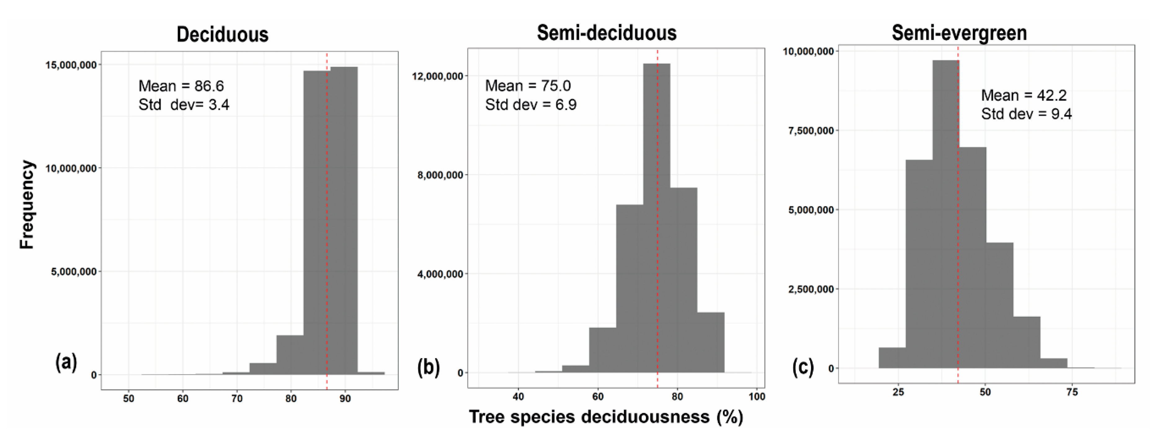
3.1. Patterns of Tree Species Deciduousness

Summary statistics of plot-level tree species deciduousness calculated in the field in each study site are shown in Table 2. The percentage of deciduous species was highly variable in the Yucatan Peninsula. El Palmar site (the driest site) showed the highest mean values of deciduous species (91.5%) and the lowest range of values (65.9%–100%), whereas FCP (the wettest site) showed the lowest mean deciduousness (43.3%). Kaxil Kiuic showed an intermediate mean value (80.4%) of deciduousness and, like FCP, a very wide range.

3.2. Modeling Tree Species Deciduousness and Model Validations

The fitted random forest models used to estimate tree species deciduousness from three sets of explanatory variables (spectral variables, texture measurement, and the combination of both data sets), indicated moderate percentage of tree species deciduousness variance explained by the models with R2 values from 0.56 to 0.60 and a RMSE between 16.2% and 16.9% (Table 3). The model that included all explanatory variables performed better than the models that used exclusively the spectral variables or the texture metrics. There was no significant spatial autocorrelation (p > 0.05) of the residuals of the three models. On the other hand, the accuracy assessment using validation data for the best fitted model (the one that combined both sets of variables) performed very well as indicated by the high R2 value (0.67) and low error (relative RMSE = 14.4%) (Figure 2).

3.3. Relationships between Predictor Variables and Tree Species Deciduousness

The most important variables for predicting tree species deciduousness on the best random forest regression model are shown in Figure 3a. They were ranked using the increased mean square error measured in percentage values (% Inc MSE). The Inc MSE represents the increase of the error prediction when the variable is removed from the model. Higher Inc. MSE indicates greater variable importance. The most important predictors include NIR band, some texture metrics (NDVI mean, NIR correlation, NIR variance), the NDVI, as well as the visible bands and the SMA deciduousness fraction.
We found significant correlations between plot-level tree species deciduousness and the most important variables in the model (Figure 3b, p < 0.001). The reflectance values of the NIR band were negatively correlated to tree species deciduousness, while the visible band (blue, green, and red) showed positive associations with deciduousness. On the other hand, deciduousness showed a negative association with NDVI and positive correlation with SMA deciduous fraction. Finally, most of the texture measures that quantify homogeneity (NIR correlation, NIR Mean, NIR homogeneity, red mean, red correlation, green mean) were positively associated with tree species deciduousness. However, some of the texture measures that quantify homogeneity were negatively associated with deciduousness (NDVI mean and SMA mean). Additionally, the texture measures that quantify heterogeneity were negatively associated with deciduousness (SMA variance, NDVI variance, and NIR variance).

3.4. Variance Partitioning of Tree Species Deciduousness

Total variance explained by the random forest model that combined all the explanatory groups of variables was 60% (Figure 4). The two groups of variables jointly (“Shared” in Figure 4) explained most of deciduousness variance (55%). The texture explanatory variables exclusively explained more variation in deciduousness (4%) than the spectral data (spectral band, NDVI, and SMA deciduousness fraction) exclusively (1%).

3.5. Mapping the Spatial Distribution of Tree Species Deciduousness and Its Uncertainty

Using the random forest (RF) models, we mapped the canopy-level deciduousness for each site in the study area (Figure 5). The frequency distribution of deciduousness in the three study sites showed a consistency with the patterns observed in the field, having higher mean values of tree species deciduousness in the El Palmar site (86.6%) compared to the other two sites with mean values of 75.0 and 42.2% respectively for Kaxil Kiuic and FCP sites. The variation of tree species deciduousness estimates has an opposite pattern, having higher standard deviation in the semi-evergreen forest compared with the deciduous forest with values of 9.4 and 3.4% respectively (Figure 6). Finally, the uncertainty maps varied widely across the three vegetation types. The uncertainties in most of the area covered by El Palmar and Kaxil Kiuic were below 20% of the coefficient of variation (CV), whereas the uncertainties were close to 60% of CV in most of the areas covered by the FCP site (Figure 7).

4. Discussion

To our knowledge, this is the first study to map the canopy phenology of tropical dry forests and its uncertainty, as well as the spatial variation in deciduousness at coarse spatial scales, using satellite information at a fine spatial resolution (10 m). Most studies mapping deciduousness have used satellite imagery data with coarse spatial resolutions such as 250 m, 500 m, and 1 km [45]. A major finding of this research is that spectral bands, vegetation indices, spectral unmixing fractions, and texture metrics from high-resolution imagery are good predictors of tree species deciduousness of tropical dry forests along an environmental gradient that covers the most important forest ecosystems in the Yucatan Peninsula. The fit of our best model (R2 = 0.60) was comparable to that of the few previous studies relating high-resolution satellite imagery data and deciduousness: R2 = 0.71 in Mediterranean natural habitats [46] and R2 = 0.55 in a gradient of evergreen to deciduous tropical forests in Africa [19]. Moreover, the accuracy assessment of the best fitted model showed a good performance after validation using an independent data set with a deciduousness estimation accuracy of R2 = 0.67 and RMSE = 14.4% (Table 3 and Figure 2).
Knowledge of the spatial distribution of deciduousness is of paramount importance for the conservation, restoration, management, and ecosystem modeling of tropical dry forests because deciduousness exerts an important control on carbon and water fluxes [47,48]. This is because many tree species in tropical dry forests exhibit a distinctive leaf-deciduous phenology to cope with seasonal drought, which affects the recruitment and growth of tree species and hence the productivity and biogeochemical cycles of these forests [49].
The patterns of the spatial distribution of deciduousness in the three types of tropical dry forest mapped in this study (Figure 5 and Figure 6) are consistent with the increase in precipitation, soil depth, and slight decrease in temperature from the northwest to the southeast of the Yucatan Peninsula [16,27]. In line with this gradient, deciduousness decreased from the northwest to the southeast, with mean values of 86.6%, 75.0%, and 42.2% respectively for deciduous, semi-deciduous, and semi-evergreen forests (Figure 6). This deciduousness gradient is also consistent with the inverse gradient in aboveground biomass for the same area, with mean values of 69.3, 100.4, and 127.5 Mg ha−1 for each type of forest respectively [50].
Tree species deciduousness showed medium to high correlations with the reflectance of visible and NIR bands, the NDVI, the SMA deciduous fraction, and several texture metrics which were opposite to those reported for photosynthetically active vegetation (Figure 3). More specifically, the deciduousness of crowns was positively related with the reflectance of the visible bands (blue, green, and red) which are negatively associated with chlorophyll absorption used for discriminating photosynthetically active vegetation [51,52]. Similarly, the NIR band and NDVI were negatively correlated to deciduousness showing an opposite pattern to vegetation during active greening [19,53]. Conversely, we found a positive association with the SMA deciduous fraction, which differentiates the non-photosynthetic vegetation fraction.
The negative correlation between texture measures of heterogeneity and deciduousness (Figure 3) can be interpreted in terms of the varying degrees of deciduousness shown by tropical forests [8,11], since the presence of forest patches with deciduous canopy trees mixed with patches of trees with green forest canopies can be captured by texture metrics of heterogeneity calculated from high-resolution imagery. Thus, high values of heterogeneity (representing areas with a mixture of deciduous and green canopies within a 1 ha sampling plot) are expected to be negatively associated with deciduousness. On the other hand, tree species deciduousness showed contrasting associations with texture measures of homogeneity. This result could be related to both ends of the gradient of deciduousness. At one end, most areas in the deciduous forest site (Figure 5a) are homogeneous with more than 80% of deciduous species, and showed a positive correlation between deciduousness and texture metrics of homogeneity. At the other extreme, in the semi-evergreen forest site (Figure 5c), there are homogeneous 1 ha areas dominated by green canopy forest, where texture measures of homogeneity were negatively correlated with deciduousness.
These results reveal the importance of using texture metrics for estimating deciduousness. The results also concur with other studies mapping different vegetation attributes of the forest using texture metrics with high-resolution imagery, such as forest structure [22,54], species diversity [55,56], leaf area index [57], and above ground biomass [58]. The variance partition analysis further highlighted the importance of using texture metrics in addition to spectral data. Combining information from spectral data and texture metrics of Sentinel-2 increased the variation of deciduousness explained by the model fit (R2 = 0.60) compared to the models using spectral data exclusively (R2 = 0.56) or texture variables only (R2 = 0.59). Moreover, texture data had higher exclusive contribution to explain variation in tree species deciduousness (4%) compared to spectral variables (1%). However, most of the variation in deciduousness (55%) was explained by the shared contribution of both sets of variables.
Interestingly, the gradient of deciduousness present in the Yucatán peninsula was inversely associated with estimation errors. Thus, the coefficient of variation in deciduousness increased from the northwest to the southeast—opposite to the gradient of deciduousness (Figure 7). This result indicates that the deciduous and semi-deciduous forests are more homogenous in terms of deciduousness (most species are deciduous; Figure 5 and Figure 6), likely reflecting a stronger environmental filtering (in terms of water availability) compared to the semi-evergreen forest, where more benign conditions allow a greater mixture of leaf-phenology strategies. Such a mixture likely occurs at a fine spatial scale, since the estimation errors of the most heterogeneous (semi-evergreen) site were highest despite the use of texture measures capturing heterogeneity in deciduousness. In other words, during the dry season, evergreen trees in the semi-evergreen forest are likely surrounded by trees with varying degrees of deciduousness [8]. Therefore, the 10 m imagery resolution of this study may capture heterogeneity in deciduousness among forest patches, but not among individual tree crowns within patches. Very high-resolution imagery (<1 m resolution) has been used to detect variation in crown size and crown density [23] and may be necessary to discriminate between evergreen and deciduous tree crowns. In the same study region, Reyes-Palomeque et al. [59] used texture metrics from orthophotos (<1 m resolution) to improve the estimation accuracy of above ground biomass to levels comparable to those obtained from LiDAR data thanks to a finer distinction of forest canopy grain. Therefore, the use of very high-resolution imagery should be considered when estimating the spatial distribution of deciduousness on future research, particularly in complex heterogeneous areas such as the semi-evergreen forest of this study.

5. Conclusions

We presented an approach for mapping the percentage of deciduous species in tropical dry forests using reflectance of visible and NIR bands, the NDVI, the SMA deciduous fraction, and several texture metrics of high-resolution imagery (10 m). We found that the approach that combined spectral information with texture metrics increased the percentage of variation in deciduousness explained, compared to the approach that used exclusively spectral information or texture data. These results reveal the importance of using texture metrics for estimating deciduousness because they can capture variation among forest patches with different degrees of deciduous. Interestingly, the highest prediction errors corresponded to the semi-evergreen forest site, which has the most complex, heterogeneous, and diverse vegetation structure and composition. This suggests that very high-resolution imagery may be necessary to account for fine-scale variation in deciduousness at the tree crown level inside the 10 m patches identified in this study. Finally, we obtained the first spatially continuous map of forest tree species deciduousness in the Yucatan Peninsula, showing that the spatial distribution of deciduousness follows the precipitation gradient.

Supplementary Materials

The following are available online at https://www.mdpi.com/1999-4907/11/11/1234/s1, Table S1: Foliar habit of the species recorded in this study.

Author Contributions

Conceptualization, A.H.H.-R. and J.L.H.-S.; Methodology, A.H.H.-R., N.B.S. and J.L.H.-S.; Investigation, A.H.H.-R. and J.L.H.-S.; Data Curation, A.H.H.-R. and F.T.-D.; Writing—Original Draft Preparation, A.H.H.-R. and J.L.H.-S.; Writing-Review & Editing, A.H.H.-R., J.M.D., C.R.-G., N.B.S., J.S.P., F.T.-D. and J.L.H.-S.; Funding Acquisition, J.L.H.-S. All authors have read and agreed to the published version of the manuscript.

Funding

The study was financially supported by CICY and Ecometrica LTD and the United Kingdom Space Agency as part of the project Forests 2020. This study is part of the first author’s Ph.D. dissertation which was supported by a grant from IICA-CONACYT.

Acknowledgments

We thank James Callaghan and Kaxil Kiuic A. C. for providing logistic support and the community of Xkobenhaltun for their continued support with fieldwork. Finally, we want to thank FiligonioMay-Pat for their help in the fieldwork and their identification of foliar habitat of the species.

Conflicts of Interest

No potential conflict of interest was reported by the authors.

References

  1. Miles, L.; Newton, A.C.; DeFries, R.S.; Ravilious, C.; May, I.; Blyth, S.; Kapos, V.; Gordon, J.E. A Global Overview of the Conservation Status of Tropical Dry Forests. J. Biogeogr. 2006, 33, 491–505. [Google Scholar] [CrossRef]
  2. Griscom, H.P.; Ashton, M.S. Restoration of Dry Tropical Forests in Central America: A Review of Pattern and Process. For. Ecol. Manag. 2011, 261, 1564–1579. [Google Scholar] [CrossRef]
  3. Murphy, P.G.; Lugo, A.E. Ecology of Tropical Dry Forest. Annu. Rev. Ecol. Syst. 1986, 17, 67–88. [Google Scholar] [CrossRef]
  4. Eamus, D.; Prior, L. Ecophysiology of Trees of Seasonally Dry Tropics: Comparisons among Phenologies. Adv. Ecol. Res. 2001, 32, 113–197. [Google Scholar] [CrossRef]
  5. Lebrija-Trejos, E.; Pérez-GarcíA, E.A.; Meave, J.A.; Bongers, F.; Poorter, L. Functional Traits and Environmental Filtering Drive Community Assembly in a Species-Rich Tropical System. Ecology 2010, 91, 386–398. [Google Scholar] [CrossRef] [PubMed] [Green Version]
  6. Lohbeck, M.; Lebrija-Trejos, E.; Martínez-Ramos, M.; Meave, J.A.; Poorter, L.; Bongers, F. Functional Trait Strategies of Trees in Dry and Wet Tropical Forests Are Similar but Differ in Their Consequences for Succession. PLoS ONE 2015, 10, e0123741. [Google Scholar] [CrossRef] [PubMed] [Green Version]
  7. Kikuzawa, K.; Lechowicz, M.J. Ecology of Leaf Longevity. Ecol. Res. Monogr. 2011. [Google Scholar] [CrossRef]
  8. Bohlman, S.A. Landscape Patterns and Environmental Controls of Deciduousness in Forests of Central Panama. Glob. Ecol. Biogeogr. 2010, 19, 376–385. [Google Scholar] [CrossRef]
  9. Singh, K.P.; Kushwaha, C.P. Deciduousness in Tropical Trees and Its Potential as Indicator of Climate Change: A Review. Ecol. Indic. 2016, 69, 699–706. [Google Scholar] [CrossRef]
  10. Zhou, G.; Houlton, B.Z.; Wang, W.; Huang, W.; Xiao, Y.; Zhang, Q.; Liu, S.; Cao, M.; Wang, X.; Wang, S.; et al. Substantial Reorganization of China’s Tropical and Subtropical Forests: Based on the Permanent Plots. Glob. Chang. Biol. 2014, 20, 240–250. [Google Scholar] [CrossRef]
  11. Condit, R.; Watts, K.; Bohlman, S.A.; Pérez, R.; Foster, R.B.; Hubbell, S.P. Quantifying the Deciduousness of Tropical Forest Canopies under Varying Climates. J. Veg. Sci. 2000, 11, 649–658. [Google Scholar] [CrossRef] [Green Version]
  12. Williams, L.J.; Bunyavejchewin, S.; Baker, P.J. Deciduousness in a Seasonal Tropical Forest in Western Thailand: Interannual and Intraspecific Variation in Timing, Duration and Environmental Cues. Oecologia 2008, 155, 571–582. [Google Scholar] [CrossRef] [PubMed] [Green Version]
  13. Kushwaha, C.P.; Tripathi, S.K.; Singh, G.S.; Singh, K.P. Diversity of Deciduousness and Phenological Traits of Key Indian Dry Tropical Forest Trees. Ann. For. Sci. 2010, 67, 310. [Google Scholar] [CrossRef] [Green Version]
  14. Gond, V.; Fayolle, A.; Pennec, A.; Cornu, G.; Mayaux, P.; Camberlin, P.; Doumenge, C.; Fauvet, N.; Gourlet-Fleury, S. Vegetation Structure and Greenness in Central Africa from Modis Multi-Temporal Data. Philos. Trans. R. Soc. B Biol. Sci. 2013, 368, 20120309. [Google Scholar] [CrossRef] [Green Version]
  15. Ouédraogo, D.Y.; Fayolle, A.; Gourlet-Fleury, S.; Mortier, F.; Freycon, V.; Fauvet, N.; Rabaud, S.; Cornu, G.; Bénédet, F.; Gillet, J.F.; et al. The Determinants of Tropical Forest Deciduousness: Disentangling the Effects of Rainfall and Geology in Central Africa. J. Ecol. 2016, 104, 924–935. [Google Scholar] [CrossRef]
  16. Valdez-Hernández, M.; González-Salvatierra, C.; Reyes-García, C.; Jackson, P.C.; Andrade, J.L. Physiological Ecology of Vascular Plants. In Biodiversity and Conservation of the Yucatan Peninsula; Springer: Cham, Switzerland, 2015. [Google Scholar] [CrossRef]
  17. Cuba, N.; Lawrence, D.; Rogan, J.; Williams, C.A. Local Variability in the Timing and Intensity of Tropical Dry Forest Deciduousness Is Explained by Differences in Forest Stand Age. GIScience Remote Sens. 2018, 55, 437–456. [Google Scholar] [CrossRef]
  18. Ganguly, S.; Friedl, M.A.; Tan, B.; Zhang, X.; Verma, M. Land Surface Phenology from MODIS: Characterization of the Collection 5 Global Land Cover Dynamics Product. Remote Sens. Environ. 2010, 114, 1805–1816. [Google Scholar] [CrossRef] [Green Version]
  19. Viennois, G.; Barbier, N.; Fabre, I.; Couteron, P. Multiresolution Quantification of Deciduousness in West-Central African Forests. Biogeosciences 2013, 10, 6957–6967. [Google Scholar] [CrossRef]
  20. Cuba, N.; Rogan, J.; Christman, Z.; Williams, C.A.; Schneider, L.C.; Lawrence, D.; Millones, M. Modelling Dry Season Deciduousness in Mexican Yucatán Forest Using MODIS EVI Data (2000-2011). GIScience Remote Sens. 2013, 50, 26–49. [Google Scholar] [CrossRef]
  21. Cuba, N.; Rogan, J.; Lawrence, D.; Williams, C. Cross-Scale Correlation between in Situ Measurements of Canopy Gap Fraction and Landsat-Derived Vegetation Indices with Implications for Monitoring the Seasonal Phenology in Tropical Forests Using MODIS Data. Remote Sens. 2018, 10, 979. [Google Scholar] [CrossRef] [Green Version]
  22. Pasher, J.; King, D.J. Multivariate Forest Structure Modelling and Mapping Using High Resolution Airborne Imagery and Topographic Information. Remote Sens. Environ. 2010, 114, 1718–1732. [Google Scholar] [CrossRef]
  23. Ploton, P.; Barbier, N.; Couteron, P.; Antin, C.M.; Ayyappan, N.; Balachandran, N.; Barathan, N.; Bastin, J.F.; Chuyong, G.; Dauby, G.; et al. Toward a General Tropical Forest Biomass Prediction Model from Very High Resolution Optical Satellite Images. Remote Sens. Environ. 2017, 200, 140–153. [Google Scholar] [CrossRef]
  24. Rzedowski, J. Vegetacion de Mexico; Comisión Nacional para el Conocimiento y Uso de la. Biodiversidad (CONABIO): Mexico City, Mexico, 2006. [Google Scholar]
  25. Islebe, G.A.; Schmook, B.; Calmé, S.; León-Cortés, J.L. Introduction: Biodiversity and Conservation of the Yucatán Peninsula, Mexico. In Biodiversity and Conservation of the Yucatan Peninsula; Springer: Cham, Switzerland, 2015. [Google Scholar] [CrossRef]
  26. Duch, G. La Conformación Territorial Del Estado de Yucatán, Los Componentes Del Medio Físico; Universidad Autonoma Chapingo. Centro Regional de la Península de Yucatán: Texcoco, México, 1988. [Google Scholar]
  27. Orellana, R.; Espadas, C.; Conde, C.; Gay, C. Atlas Escenarios de Cambio Climático En La Península de Yucatán; Centro de Investigación Científica de Yucatán (CICY): Mérida, México, 2009. [Google Scholar]
  28. Bautista-Zúñiga, F.; Batllori-Sampedro, E.; Ortiz-Pérez, M.A.; Palacio-Aponte, G.; Castillo-González, M. Geoformas, Agua y Suelo En La Península de Yucatán. In Naturaleza y Sociedad en el área Maya. Pasado, Presente y Futuro; Colunga, P., Larqué, A., Eds.; Centro de Investigación Científica de Yucatán (CICY): Mérida, México, 2003; pp. 21–36. [Google Scholar]
  29. Miranda, F.; Hernández-X, E. Los Tipos de Vegetación de México y Su Clasificación. Bot. Sci. 1963, 28, 29–179. [Google Scholar] [CrossRef]
  30. CONAFOR [Comisión Nacional Forestal]. Inventario Nacional y de Suelos. Manual y Procedimientos Para El Muestreo de Campo; CONAFOR: Zapopan, Jalisco, Mexico, 2013. [Google Scholar]
  31. Hernández-Stefanoni, J.L.; Reyes-Palomeque, G.; Castillo-Santiago, M.Á.; George-Chacón, S.P.; Huechacona-Ruiz, A.H.; Tun-Dzul, F.; Rondon-Rivera, D.; Dupuy, J.M. Effects of Sample Plot Size and GPS Location Errors on Aboveground Biomass Estimates from LiDAR in Tropical Dry Forests. Remote Sens. 2018, 10, 1586. [Google Scholar] [CrossRef] [Green Version]
  32. Gorelick, N.; Hancher, M.; Dixon, M.; Ilyushchenko, S.; Thau, D.; Moore, R. Google Earth Engine: Planetary-Scale Geospatial Analysis for Everyone. Remote Sens. Environ. 2017, 202, 18–27. [Google Scholar] [CrossRef]
  33. Sentinel, E.S.A. User Handbook; ESA Stand. Doc. 2AD; ESA: Paris, France, 2015; p. 64. [Google Scholar]
  34. Adams, J.B.; Gillespie, A.R. Remote Sensing of Landscapes with Spectral Images; Cambridge University Press: Cambridge, UK, 2006. [Google Scholar] [CrossRef]
  35. Boardman, J.W.; Kruse, F.A.; Green, R.O. Mapping Target Signatures via Partial Unmixing of AVIRIS Data. Summ. JPL Airborne Earth Sci. Work. 1995, 1, 23–26. [Google Scholar]
  36. Exelis Visual Information Solutions. Environment for Visualizing Images (ENVI); Exelis Visual Information Solutions: Boulder, CO, USA, 2013. [Google Scholar]
  37. Haralick, R.M.; Dinstein, I.; Shanmugam, K. Textural Features for Image Classification. IEEE Trans. Syst. Man Cybern. 1973, 610–621. [Google Scholar] [CrossRef] [Green Version]
  38. Zvoleff, A. Glcm: Calculate Textures from Grey-Level Co-Occurrence Matrices (GLCMs); R-CRAN Project; 2019; Available online: https://cran.r-project.org/web/packages/glcm/index.html (accessed on 26 March 2019).
  39. Liaw, A.; Wiener, M. Classification and Regression by RandomForest. R News 2002, 2, 18–22. [Google Scholar]
  40. Breiman, L. Random Forests. Mach. Learn. 2001, 45, 5–32. [Google Scholar] [CrossRef] [Green Version]
  41. Borcard, D.; Legendre, P.; Avois-Jacquet, C.; Tuomisto, H. Dissecting the Spatial Structure of Ecological Data at Multiple Scales. Ecology 2004, 85, 1826–1832. [Google Scholar] [CrossRef] [Green Version]
  42. Freeman, E.; Frescino, T.; Moisen, G. ModelMap: An R Package for Modeling and Map Production Using Random Forest and Stochastic Gradient Boosting; USDA Forest Service, Rocky Mountain Research Station: Fort Collins, CO, USA, 2009. [Google Scholar]
  43. Zar, J. Biostatistical Analysis, 4nd ed.; Prentice Hall: Upper Saddle River, NJ, USA, 1999. [Google Scholar]
  44. Freeman, E.A.; Moisen, G.G.; Coulston, J.W.; Wilson, B.T. Random Forests and Stochastic Gradient Boosting for Predicting Tree Canopy Cover: Comparing Tuning Processes and Model Performance. Can. J. For. Res. 2015, 46, 323–339. [Google Scholar] [CrossRef] [Green Version]
  45. Adole, T.; Dash, J.; Atkinson, P.M. A Systematic Review of Vegetation Phenology in Africa. Ecol. Inform. 2016, 34, 117–128. [Google Scholar] [CrossRef]
  46. Feret, J.B.; Corbane, C.; Alleaume, S. Detecting the Phenology and Discriminating Mediterranean Natural Habitats with Multispectral Sensors-An Analysis Based on Multiseasonal Field Spectra. IEEE J. Sel. Top. Appl. Earth Obs. Remote Sens. 2015, 8, 2294–2305. [Google Scholar] [CrossRef]
  47. Xu, X.; Medvigy, D.; Powers, J.S.; Becknell, J.M.; Guan, K. Diversity in Plant Hydraulic Traits Explains Seasonal and Inter-Annual Variations of Vegetation Dynamics in Seasonally Dry Tropical Forests. New Phytol. 2016, 212, 80–95. [Google Scholar] [CrossRef] [PubMed]
  48. Restrepo-Coupe, N.; Levine, N.M.; Christoffersen, B.O.; Albert, L.P.; Wu, J.; Costa, M.H.; Galbraith, D.; Imbuzeiro, H.; Martins, G.; da Araujo, A.C.; et al. Do Dynamic Global Vegetation Models Capture the Seasonality of Carbon Fluxes in the Amazon Basin? A Data-Model Intercomparison. Glob. Chang. Biol. 2017, 23, 191–208. [Google Scholar] [CrossRef] [PubMed] [Green Version]
  49. van der Sande, M.T.; Peña-Claros, M.; Ascarrunz, N.; Arets, E.J.M.M.; Licona, J.C.; Toledo, M.; Poorter, L. Abiotic and Biotic Drivers of Biomass Change in a Neotropical Forest. J. Ecol. 2017, 105, 1223–1234. [Google Scholar] [CrossRef] [Green Version]
  50. Hernández-Stefanoni, J.L.; Castillo-Santiago, M.Á.; Mas, J.F.; Wheeler, C.E.; Andres-Mauricio, J.; Tun-Dzul, F.; George-Chacón, S.P.; Reyes-Palomeque, G.; Castellanos-Basto, B.; Vaca, R.; et al. Improving Aboveground Biomass Maps of Tropical Dry Forests by Integrating LiDAR, ALOS PALSAR, Climate and Field Data. Carbon Balance Manag. 2020, 15, 1–17. [Google Scholar] [CrossRef]
  51. Vieira, I.C.G.; De Almeida, A.S.; Davidson, E.A.; Stone, T.A.; Reis De Carvalho, C.J.; Guerrero, J.B. Classifying Successional Forests Using Landsat Spectral Properties and Ecological Characteristics in Eastern Amazônia. Remote Sens. Environ. 2003, 87, 470–481. [Google Scholar] [CrossRef]
  52. Thenkabail, P.S.; Enclona, E.A.; Ashton, M.S.; Legg, C.; De Dieu, M.J. Hyperion, IKONOS, ALI, and ETM+ Sensors in the Study of African Rainforests. Remote Sens. Environ. 2004, 90, 23–43. [Google Scholar] [CrossRef]
  53. Muldavin, E.H.; Neville, P.; Harper, G. Indices of Grassland Biodiversity in the Chihuahuan Desert Ecoregion Derived from Remote Sensing. Conserv. Biol. 2001, 15, 844–855. [Google Scholar] [CrossRef]
  54. Gallardo-Cruz, J.A.; Meave, J.A.; González, E.J.; Lebrija-Trejos, E.E.; Romero-Romero, M.A.; Pérez-García, E.A.; Gallardo-Cruz, R.; Hernández-Stefanoni, J.L.; Martorell, C. Predicting Tropical Dry Forest Successional Attributes from Space: Is the Key Hidden in Image Texture? PLoS ONE 2012, 7, e30506. [Google Scholar] [CrossRef] [PubMed] [Green Version]
  55. Viedma, O.; Torres, I.; Pérez, B.; Moreno, J.M. Modeling Plant Species Richness Using Reflectance and Texture Data Derived from QuickBird in a Recently Burned Area of Central Spain. Remote Sens. Environ. 2012, 119, 208–221. [Google Scholar] [CrossRef]
  56. George-Chacon, S.P.; Dupuy, J.M.; Peduzzi, A.; Hernandez-Stefanoni, J.L. Combining High Resolution Satellite Imagery and Lidar Data to Model Woody Species Diversity of Tropical Dry Forests. Ecol. Indic. 2019, 101, 975–984. [Google Scholar] [CrossRef]
  57. Zhou, J.; Yan Guo, R.; Sun, M.; Di, T.T.; Wang, S.; Zhai, J.; Zhao, Z. The Effects of GLCM Parameters on LAI Estimation Using Texture Values from Quickbird Satellite Imagery. Sci. Rep. 2017, 7, 7366. [Google Scholar] [CrossRef]
  58. Chen, L.; Wang, Y.; Ren, C.; Zhang, B.; Wang, Z. Optimal Combination of Predictors and Algorithms for Forest Above-Ground Biomass Mapping from Sentinel and SRTM Data. Remote Sens. 2019, 11, 414. [Google Scholar] [CrossRef] [Green Version]
  59. Reyes-Palomeque, G.; Dupuy, J.M.; Johnson, K.D.; Castillo-Santiago, M.A.; Hernández-Stefanoni, J.L. Combining LiDAR Data and Airborne Imagery of Very High Resolution to Improve Aboveground Biomass Estimates in Tropical Dry Forests. For. Int. J. For. Res. 2019, 92, 599–615. [Google Scholar] [CrossRef]
Figure 1. Location of the study area showing the three sites (a) as well as the distribution of plots for each type of tropical dry forest: deciduous (b), semi-deciduous (c), and semi-evergreen forest (d) and a false color composite of the study area using green, red, and near-infrared bands from Sentinel-2 imagery. ICM: intensive carbon monitoring, NFI: national forest inventory.
Forests 11 01234 g001
Figure 2. Model validation analyses of the best-fitted model for predicting tree species deciduousness. The graph shows predicted versus observed tree species deciduousness. The dashed red line shows 1:1 reference line and the bold line is the regression line.
Forests 11 01234 g002
Figure 3. Predictor importance ranking derived from the best random forest model. (a) The rank is based on the increase of mean square error (% Inc. MSE) when the explanatory variable is removed. (b) Pearson’s correlation coefficients between explanatory variables and tree species deciduousness measured in the field. All correlations were significant (p < 0.001).
Forests 11 01234 g003
Figure 4. Results of the variance partitioning analysis for predicting tree species deciduousness from spectral and texture information calculated from Sentinel-2 imagery. The spectral information includes reflectance of spectral band, NDVI, and SMA deciduousness fraction.
Forests 11 01234 g004
Figure 5. Maps of tree species deciduousness for each vegetation type: (a) deciduous (El Palmar), (b) semi-deciduous (Kaxil Kiuic), and (c) semi-evergreen (Felipe Carrillo Puerto: FCP). Areas in white correspond to non-forest covers, mostly agricultural lands and human settlements.
Forests 11 01234 g005
Figure 6. Frequency distribution of estimated tree species deciduousness in a 3600 km2 window of three types of tropical dry forest: deciduous (a), semi-deciduous (b), and semi-evergreen (c).
Forests 11 01234 g006
Figure 7. Deciduousness uncertainty maps for each vegetation type: (a) deciduous (El Palmar), (b) semi-deciduous (Kaxil Kiuic), and (c) semi-evergreen (Felipe Carrillo Puerto: FCP).
Forests 11 01234 g007
Table 1. Sentinel 2 multi spectral instrument images used in this study.
SiteAcquisition TimeSensor TypeTile Numbers
El Palmar24 March 2018S2AT15QYC, T15QYD, T15QZC, T15QZD
26 March 2018S2BT16QBH, T16QBJ
Kaxil Kiuic6 March 2018S2BT15QZB, T15QZC
FCP16 March 2018S2BT16QCF, T16QCG
Table 2. Summary statistics of the tree species deciduousness weighed by basal area sampled at field in 1 ha forest inventory plots, measured as percentage.
SitenMeanSDMinMaxRange
Palmar3391.57.965.9100.034.1
Kaxil Kiuic13480.414.50.0100.0100.0
FCP12143.318.20.8100.099.2
Table 3. Evaluation statistics for predicting tree species deciduousness from spectral data (bands, normalized difference vegetation index (NDVI), and spectral mixture analysis (SMA)) texture variables and both sets of data using random forest.
ModelExplanatory VariablesR2RMSE (%)
Combining spectral and texture variablesSpectral values from blue, green red, and NIR bands + NDVI + SMA deciduous fraction + Texture metrics of spectral bands, NDVI and SMA0.6016.2
Spectral variablesSpectral values from blue, green red, and NIR bands + NDVI + SMA deciduous fraction0.5616.9
Texture variablesTexture metrics of spectral bands, NDVI, and SMA0.5916.3
Publisher’s Note: MDPI stays neutral with regard to jurisdictional claims in published maps and institutional affiliations.

