Article

Assessing Habitat Suitability of Parasitic Plant Cistanche deserticola in Northwest China under Future Climate Scenarios

1
National Engineering Laboratory for Resource Development of Endangered Crude Drugs in Northwest China, Shaanxi Normal University, Xi’an 710119, China
2
School of Geography and Tourism, Shaanxi Normal University, Xi’an 710119, China
3
College of Life Sciences, Shaanxi Normal University, Xi’an 710119, China
*
Authors to whom correspondence should be addressed.
Forests 2019, 10(9), 823; https://doi.org/10.3390/f10090823
Submission received: 30 June 2019 / Revised: 10 September 2019 / Accepted: 17 September 2019 / Published: 19 September 2019
(This article belongs to the Special Issue Impact of Land Use Change on Forest Biodiversity)

Abstract

:
Cistanche deserticola Ma, a perennial parasitic herb of family Orobanchaceae, is mainly parasitic on the roots of the Haloxylon ammodendron Bunge. In view of this special parasitic relationship, we applied random forest (RF) model to forecast potential geographic distribution, and developed a comprehensive habitat suitability model by integrating bioclimatic and soil factors to assess the suitable distribution of C. deserticola and H. ammodendron across China in 2050s and 2070s under RCP2.6, RCP4.5, and RCP8.5, respectively. We modeled the core potential geographic distribution of C. deserticola by overlaying the distribution of these two species, and analyzed the spatial distribution pattern and migration trend of C. deserticola by using the standard deviational ellipse. In addition, we evaluated the accuracy of RF model through three evaluation indexes, and analyzed the dominant climate factors. The results showed that the core potential distribution areas of C. deserticola are distributed in the Xinjiang Uygur Autonomous Region, the junction of Shaanxi–Gansu–Ningxia provinces, and the Inner Mongolia Autonomous Region. The spatial dispersion would intensify with the increasing of emission scenarios, and the geographical habitat is moving towards higher latitude. Among the three evaluation indexes, the area under the ROC curve (AUC) and True Skill Statistic (TSS) have better assessment results. The main bioclimatic factors affecting the distribution are min temperature of coldest month (Bio6), annual precipitation (Bio12), precipitation of wettest month (Bio13), precipitation of wettest quarter (Bio16), and precipitation of warmest quarter (Bio18), among which the importance of precipitation factors is greater than temperature factors. More importantly, the results of this study could provide some guidance for the improvement of desert forest system, the protection of endangered species and the further improvement of the ecological environment.

1. Introduction

With the global warming, more and more attention has been paid to the impact and assessment of climate change by governments and scientists. The Intergovernmental Panel on Climate Change (IPCC) Fifth Assessment report (AR5) shows that the global average surface temperature are expected to rise about 0.3 °C–4.8 °C by 2100 due to the further increases of greenhouse gases in the atmosphere [1]. The future climate change of China is consistent with the global projections, which means that the warming trend in the north is more obvious than that in the south [2]. The relationship between species and environment is the core of studying biology and climate. Climate change will inevitably lead to changes in the species’ habitats distribution, and species are also shifting their ranges at an unprecedented rate through environmental change [3,4,5]. Studies have found that some species may migrate to high latitude and altitude areas [6,7,8]. Climate change directly or indirectly affects the spatial and temporal distribution pattern of species, especially for the growth and distribution of endangered species [9,10,11,12,13]. It may break the ecological balance of life on the earth and increase the risk of extinction of endangered species to a certain extent.
Maintaining long-term management strategies for endangered or rare species requires information on the potential distribution and relative abundance under current and future climate scenarios [14]. Species distribution models (SDMs) can provide information in this area, so it has been widely applied to the study of conservation area planning, and the impact of climate change on species distribution. At present, the study of SDMs has carried out climate change on animals [15,16,17,18], plants [19,20], landscape ecology [21], swamp vegetation [22], Chinese medicinal materials [23], and so on. Many algorithms have been applied to the construction of SDMs. Researchers need to choose different model algorithms for different modeling purposes, species niche characteristics and the basis of modeling data. Generally speaking, SDMs can be divided into four categories: threshold-based model (surface range envelope, SRE), regression-based model (generalized linear model (GLM), generalized boosting model (GBM), multiple adaptive regression splines (MARS)), classification-based model (generalized add model (GAM), classification tree analysis (CTA), flexible discriminant analysis (FDA)), and machine learning-based model (random forest (RF), artificial neural network (ANN), Maximum entropy (MaxEnt)) [24]. Among them, MaxEnt model has been widely used to predict the potential distribution pattern of species [25,26,27]. In recent years, RF model has been developed in the field of bioinformatics [28], remote sensing of earth science [29], land use [30], and has been paid more and more attention and applied in the study of species distribution prediction [31,32,33]. By comparing the multiple logistic regression technique in generalized linear modeling (GLM) with RF models, the prediction performance of the RF model is higher [31]. Similarly, using the SDMs of CTA, RF, MARS, FDA, GLM, GBM, GAM, and ANN to predict the global suitability distribution of Corbicula fluminea (Müller, 1744), the best modeling effect of RF is obtained [34]. Besides, the present and future potential distribution of 13 species of Heliotropium were simulated by eight models within a holistic prediction framework, it was also found that the RF model had the best performance [35]. In the case of insufficient sample size, RF model can use the measured values to generate the predicted data by classification and regression, and handle the data abnormity freely to some extent. The advantage of RF algorithm is that the model performs best in predicting species distribution and is becoming more mature for forecasting factors.
Cistanche deserticola Ma, a perennial parasitic herb of family Orobanchaceae, is commonly known as ‘Desert Ginseng’ and also is an endemic species of Cistanche Hoffmg. Et Link grown in arid areas of the northwest China. The suitable growth environment of C. deserticola is dry with low rainfall, large evaporation, long sunshine hours, and large temperature difference between day and night [36]. It is a precious traditional Chinese medicine and has the functions of enhancing immunity, anti-fatigue, anti-aging, tonifying yang, nourishing essence, and blood [37,38]. Generally, the seeds of C. deserticola move downward along the interstice of sand grains after landing, and germinate under the inducement of their secretions after encountering the root of the host plant. The germinated seeds fuse directly with the host roots to form a small tumor. When enough nutrients are absorbed, the plants of C. deserticola grow from these tumors. It is conceivable that the success rate of this parasitic method is very low, but the natural population of C. deserticola can be maintained without disturbing the external environment. Now, C. deserticola has been included in the Pharmacopoeia of the People’s Republic of China (2015), and belongs to a national second class protected plants which has been listed in the Convention on International Trade in Endangered Species of Wild Fauna (CITES) in Appendix II (https://cites.org/eng/app/appendices.php).
Haloxylon ammodendron Bunge, a perennial shrub of family Chenopodiaceae, is the main host of C. deserticola. It plays an important role in the maintenance of the structure and function of the whole ecosystem, improving vegetation, curbing desertification, reducing wind speed, and meliorating the forest microclimate [39,40]. C. deserticola is mainly parasitic on the roots of H. ammodendron to absorb carbohydrate, minerals, and even water, because it cannot perform photosynthesis itself [41,42]. Recent studies paid more attention to the interaction between C. deserticola and its host H. ammodendron [43,44]. Under the intervention of external factors, the roots of H. ammodendron were often exposed, which resulted in excessive water loss and death, further affecting the growth of C. deserticola. The desertification process of C. deserticola and H. ammodendron will be intensified, leading to severe damage to resources [45]. Therefore, effective protection is required to protect the habitats of C. deserticola.
Based on sample data, this paper analyzed the comprehensive habitat distribution in the future climate scenarios of C. deserticola (Figure 1). The objectives of this study consists of five main aspects: (1) evaluate the accuracy of RF model by three evaluation indexes; (2) built a comprehensive habitat suitability model to predict the potential future geographic distribution of C. deserticola and H. ammodendron by considering the limitation of soil conditions; (3) analysis of the dominant climate factors affecting the distribution of C. deserticola; (4) model the core potential geographic distribution of C. deserticola by superimposing the distribution of these two species; (5) analyze the spatial distribution pattern and migration trends of C. deserticola in the future climate change, based on the directional distribution module in ArcGIS. The results of this study will provide some guidance for the division of Chinese herbal medicines and provide the corresponding countermeasures for improving the ecological environment.

2. Methods

Figure 1 illustrates the habitat suitability assessment workflow. The specific steps are as followed.

2.1. Sampling and Area

Sample data of C. deserticola and H. ammodendron were collected from the Global Biodiversity Information Facility (https://www.gbif.org); Herbarium, Institute of Botany, Chinese Academy of Sciences (http://pe.ibcas.ac.cn); Chinese Nature Herbarium (http://www.nature-museum.net); Chinese Virtual Herbarium (http://www.cvh.ac.cn); Chinese Natural Reserve Specimen Resource Sharing Platform (http://www.papc.cn); and related documents. Eliminating a small number of data with duplicate and inaccurate location records, we got 68 C. deserticola distribution points, and 187 H. ammodendron distribution points (Figure 2).
The research area was determined according to the distribution range of the species points, including the Xinjiang Uygur Autonomous Region, parts of the Inner Mongolia Autonomous Region, Gansu, Qinghai, the Ningxia Hui Autonomous Region, and Shaanxi province. The counties and topographical units involved in the study area (Figure 2).

2.2. Environmental Variables

To describe the environmental conditions, we selected 19 bioclimatic variables (Bio1–Bio19) and 8 soil variables (Table 1). The bioclimatic variables were downloaded BCC_CSM1.1 (Beijing Climate Centre Climate System Modelling version 1.1) data at a resolution of 30″ (approximately 1 km2) from the Worldclim datasets (http://www.worldclim.org). The future data includes two time periods, the 2050s (average for 2041–2060) and the 2070s (average for 2061–2080). The new greenhouse gas emission scenario “representative concentration pathways, RCPs” released by IPCC AR5 puts forward that anthropogenic greenhouse gas emissions are mainly driven by population density, economic development, way of life and production, energy development, land use, and climate policies, etc. According to the atmospheric conditions, air pollutant concentration and land use types caused by greenhouse gas emissions in the 21st century, RCPs are classified into one strict mitigation scenario (RCP2.6), two moderate emission scenarios (RCP4.5 and RCP6.0), and one high greenhouse gas emission scenario (RCP8.5). In this study, RCP2.6, RCP4.5, and RCP8.5 were selected for modeling [1]. Autocorrelation among predictors may hamper the analysis of species-environment relationships in multiple regression settings. Then, we calculated the Pearson correlation coefficients (r) among the 19 bioclimatic variables in ArcGIS 10.2 (http://www.esrichina.com.cn/). If a pair of variables were strongly correlated (|r|>0.8), one of the variables was removed to avoid the prediction error induced by multicollinearity among environmental variables. We finally elected 10 bioclimatic variables to conduct model (Table 1).
Soil provides necessary space and nutrients for the survival of plants. Among the soil variables, the soil type (ST) variables was the 1:1 million soil database of China from the Data Center for Resources and Environmental Sciences, Chinese Academy of Sciences (RESDC, http://www.resdc.cn). The other soil data were derived from the Harmonized World Soil Database (HWSD, http://www.fao.org/soils-portal/). In this study, the soil variables were assumed to remain unchanged over the two future periods. All environmental variables are inserted into a resolution of 1 km2 and converted to American Standard Code for Information Interchange (ASCII) format by ArcGIS 10.2.

2.3. RF Model Setting

In this study, we selected the random forests algorithm based on the ‘biomod2’ package provided by the R software to predict the potential geographic distribution area of C. deserticola and H. ammodendron in the future. The biomod2 modeling package is developed by R for constructing species distribution models [46,47]. It can simulate the species distribution area by developing a single model or combining multiple models, explore the dynamic relationship between species spatial distribution and environmental factors, and calibrate and evaluate the model. Random forests (RF) model is a new approach to classification through machine learning and integration. It is a classifier with many decision trees. The RF model in biomod2 invokes random forest codes for classification and regression integration, and sets bagging and boosting algorithms to optimize the model, hence, it has strong practicability and low error [48,49,50]. There are two main steps in developing the RF model. Firstly, based on bootstrap method, k samples are randomly and playback extracted from the training set data as the training set of the classification tree. Secondly, m feature subsets are randomly selected from M features of each sample to prepare for classification. Bagging is used to input the sample data into each tree for classification, voting for several weak classification results, and finally forming a strong classification result [49].
The input data of RF includes species presence points, pseudo-presence points, and 10 bioclimatic variables related to species distribution. We used the created random points module created in the management tools to generate 1500 pseudo-presence points based on ArcGIS 10.2. The data of presence points and pseudo-presence points are randomly extracted and reproduced to obtain three sets of unified data. 75% of the point data in each group are trained, and 25% are tested to evaluate the accuracy of the predictions. In addition, every single model is constructed and operated four times to build six scenarios based on the three RCPs in the two future time periods. In this study, we used three evaluation indicators to assess model performance, namely area under the ROC curve (AUC) [51], Cohen’s KAPPA (KAPPA) [52], and True Skill Statistic (TSS) [53]. These evaluation indicators are dimensionless quantities. The evaluation result of the threshold is from 0 to 1, where a higher number indicates higher accuracy of the model (Table 2). According to the statistical value of the evaluation index, the optimal model is selected and the prediction results are converted into binary layers with a range of 0–1.

2.4. Comprehensive Habitat Suitability (CHS) Model

Soil variables provide important information on restricting the distributions of species. Based on the MaxEnt 3.3.3 (http://homepages.inf.ed.ac.uk/lzhang10/maxent.html), the restriction model of soil variables was constructed by using the eight soil variable data and the distribution data of C. deserticola and H. ammodendron. The model runs randomly by selecting 75% of the points to train the model, and 25% to test and validate the model. Ten replications and 10,000 mix number of background points were set to reduce uncertainty. Finnally, we selected the model with the highest performance through AUC, and divided the suitability index by the threshold value of 0.5 into two categories: suitable (≥ 0.5) and unsuitable (< 0.5).
Therefore, based on the prediction model of bioclimatic variables as well as the restriction model of soil variables, we built the comprehensive habitat suitability model to assess the distribution of C. deserticola and H. ammodendron (Equation (1))
C H S i = B T i × S i
where CHSi is the comprehensive habitat suitability index in each evaluation grid, BTi is the results value of the prediction model in each grid, Si is the results value of the restriction model for soil. The range of CHSi is (0, 1).
CHSi is mostly used to assess the comprehensive habitat distribution of species constrained by multiple factors, such as soil and vegetation, in addition to the influence of climate factors [10,54]. For further analysis, we divide CHSi into three grades: unsuitable (CHSi < 0.3), moderately suitable (0.3 ≤ CHSi < 0.5), and highly suitable (CHSi ≥ 0.5). C. deserticola, as a parasitic plant, does not naturally exist if the host disappears. H. ammodendron is the main host plant of C. deserticola. Hence, we used the raster calculator of ArcGIS to overlay the comprehensive habitat suitability results of these two species to identify the core potential geographical distribution area of C. deserticola, and also divided the area into three grades (unsuitable, moderately suitable, and highly suitable habitats).

2.5. Calculation of Spatial Pattern

In this paper, we use the directional distribution module, also known as the standard deviational ellipse (SDE) in ArcGIS to study the spatial distribution pattern of the core potential distribution area of C. deserticola (Figure 3). No data can be evenly distributed across the map, but the standard deviation ellipse can be used to measure the concentration of geographic data. Thus, using “spot map” to clarify the overall trend of the region requires a study of the central trends and dispersion of data [55]. The actual shape of the curve has remained unclear since the issue was mentioned initially by Lefever (1926). Therefore, Lefever had put forward a closed curve called the “standard deviation curve”. The shape is determined explicitly by the ratio of its minor axis to its major axis, and the major axis represents the major orientation of geographical units. The size and radius can be used to indicate the distribution density of geographical units [56]. In recent years, the standard deviational ellipse has gradually been studied in geography, which has become an important module in measuring the spatial distribution of geographical elements [57], and is often used to study the spatial variation of regional economy [58].
In order to further study the spatial pattern and migration trend of the distribution area of C. deserticola in three RCPs from 2050s to 2070s, we convert the grid map of the core potential geographic distribution area into a vector point set, and use the measuring geographic distribution module of ArcGIS to obtain the SDE, and related parameters to summarize the spatial characteristics of geographic features: central tendency, dispersion, and directional trends [59,60].
(1) Mean center ( X ¯ ,   Y ¯ ): the mean center is the average coordinates x and y of all the elements in the study area (Equation. (2)), it is very useful for studying distribution changes and central trends.
X ¯ = i = 1 n x i n   ,     Y ¯ = i = 1 n y i n
where xi and yi are the spatial position coordinates of the ith element, n is the total number of elements.
(2) Standard distance (SDEx, SDEy): a common method to measure the trend of a set of points is to calculate the standard distance in the direction of x and y, respectively. Based on the mean center as the starting point, the standard deviation of the x and y coordinates are calculated, the major axis semidiameter and the minor axis semidiameter of the ellipse are determined (Equation (3)).
S D E x = i = 1 n ( x i X ¯ ) 2 n   ,   S D E y = i = 1 n ( y i Y ¯ ) 2 n
(3) Rotation angle (θ): it refers to the angle of the north and the major axis of the ellipse (Figure 3), which is used to indicate the distribution direction of elements in the main trend (Equations (4)–(8)). In this paper, we judge the spatial pattern according to the angle α (Figure 3). According to the 16-azimuth diagram [61,62], if α less than 11.25°, we define the spatial pattern as the east–west pattern, if greater than 11.25°, it is the northeast-southwest pattern.
tan θ = A + B C
A = ( i = 1 n x ˜ i 2 i = 1 n y ˜ i 2 )
B = ( i = 1 n x ˜ i 2 i = 1 n y ˜ i 2 ) 2 + 4 ( i = 1 n x ˜ i y ˜ i ) 2
C = 2 i = 1 n x ˜ i y ˜ i
α = | θ 90 ° |
where x ˜ and y ˜ are the deviation between the coordinates of the ith element and the mean center, x ˜ = ( x i X ¯ ) , y ˜ = ( y i Y ¯ ) .
(4) Ellipticity (e): the ellipticity is defined as the ratio of the focal length to the major axis on the ellipse (Equation (9)), which ranges from 0 to 1.
e = a 2 b 2 a
where a and b represent the major axis semidiameter, and the minor axis semidiameter of the ellipse, respectively (Figure 3).
The mean center of the SDE represents the relative position of the spatial distribution of the elements. The rotation angle of reflects the main direction of the distribution. The standard distance SDEx and SDEy are the length of the major axis and minor axis. It shows the dispersion degree of elements in the main trend direction and the dispersion degree of in the second direction, respectively. The increase of SDEx indicates dispersion phenomenon in the main trend direction, while the increase of SDEx is a concentration phenomenon. The increase of SDEy indicates the dispersion in the second direction. The larger the ellipticity, the flatter the ellipse, and the more dispersed the distribution. Conversely, the smaller the ellipticity, the more concentrated the distribution.

3. Results

3.1. Model Evaluation Analysis

In this paper, 75% of the data is trained as model calibration, and 25% is set as model validation. Three indicators are used to evaluate the prediction accuracy in RF model. The results showed that the maximum and minimum evaluation values of the model were 0.975 (AUC) and 0.674 (KAAPA), respectively (Figure 4). In general, the evaluation indexes were ranked as AUC, TSS, and KAPPA, and the model prediction is successful according to the prediction accuracy.
Results showed that AUC and TSS were relatively stable among the three evaluation indexes, and there was no significant difference in the evaluation indexes under three RCPs. Under the three RCPs in 2050s, the average values of the AUC, TSS, and KAPPA were 0.967, 0.870, and 0.744 respectively. The evaluation grades of the AUC and TSS are better than KAPPA (Figure 4a). In the 2070s, the average statistical value of the three evaluation indexes is lower than those in 2050s, namely, AUC was 0.942, TSS was 0.843, and KAPPA was 0.682. However, the evaluation grade of the model was the same as that of 2050s (Figure 4b).

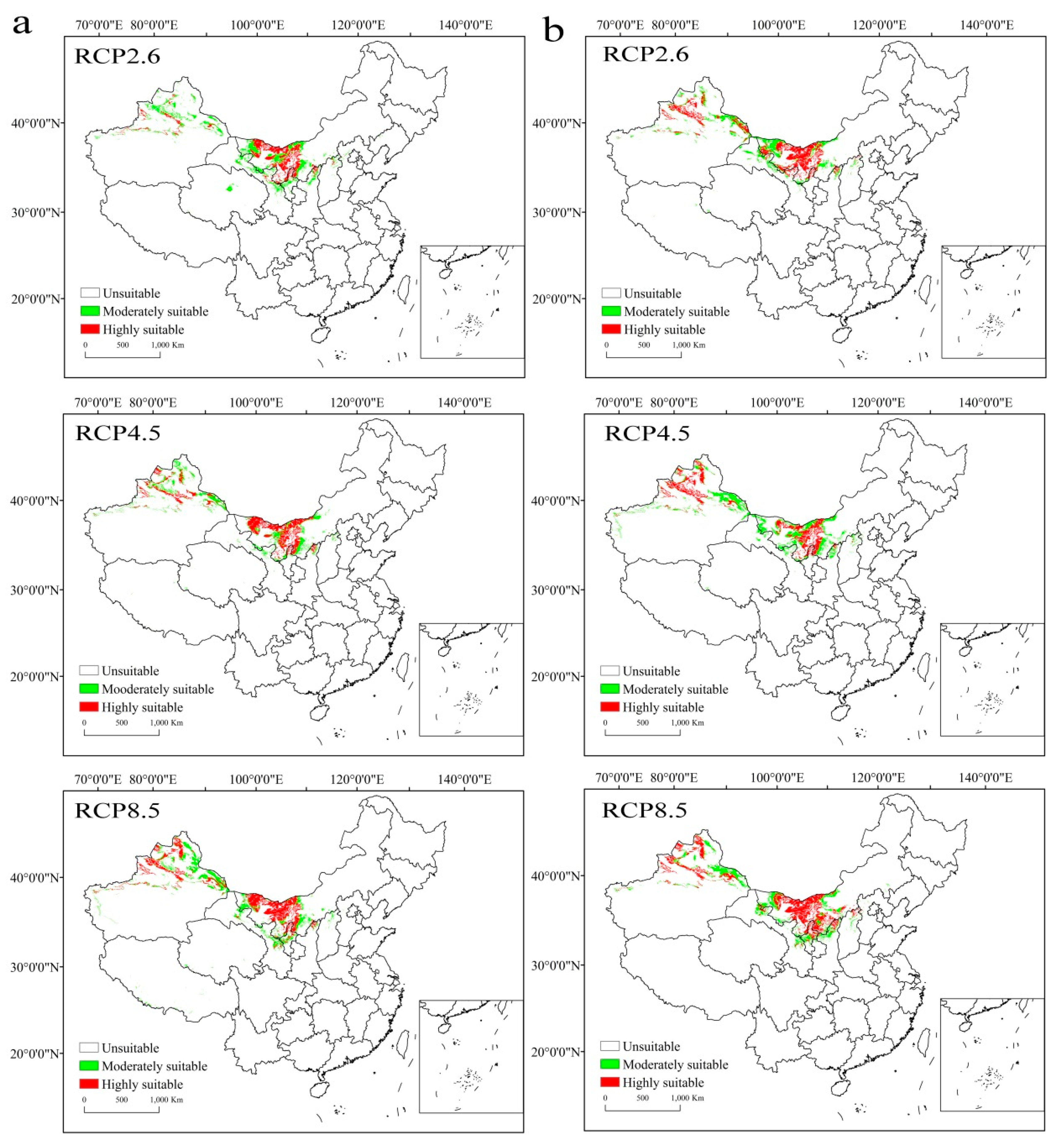
3.2. Potential Geographical Distribution of Suitable Habitats

The potential geographical distribution of C. deserticola was predicted by comprehensive habitat suitability model. The results showed that there were some differences in potential distribution habitats under different scenarios, showing a continuous and scattered distribution (Figure 5). Under RCP2.6, RCP4.5, and RCP8.5 in 2050s, moderately suitable distribution habitats of C. deserticola were mainly concentrated in the north of Tianshan Mountains, near the Junggar Basin, west of Hetao plain, northeast of Inner Mongolia Alxa League, northwest of Bayan Nur, north of Baotou city and central area of Ordos city, north of Hexi Corridor in Gansu province, and the Ningxia Hui Autonomous Region in northern China. Highly suitable mainly distributed near the Junggar Basin, west of the Hetao plain, and north of Ningxia plain (Figure 5a).
At the same RCPs in 2070s, suitable habitats of C. deserticola were distributed in the parts of the Xinjiang Uygur Autonomous Region, and the Inner Mongolia Autonomous Region on the whole (Figure 5b). However, the habitat distribution of moderately suitable increased obviously, and the highly suitable range continued to decrease from 2050s to 2070s. The moderately suitable areas were increased by 0.54%, 1.26%, and 0.83% under RCP2.6, RCP4.5, and RCP8.5, respectively. The increasing suitable habitats were mainly concentrated on increasing the regional distribution in the Badain Jaran Desert northwest region, the northwest of Hexi Corridor, Tengger Desert, and Mu Us Desert. On the contrary, the highly suitable area changes showed a reduction of 0.02%, 0.04%, and 0.09% under RCP2.6, RCP4.5, and RCP8.5, respectively. The reduced habitats were mainly concentrated in the west Junggar Basin, and in the southeastern region of Tengger Desert.

3.3. Analysis of Factor Affecting the Distribution of C. deserticola

SDMs can calculate the relative contribution rate of environmental variables and draw the factor response curve to analyze habitat threshold. After several model training, Bio6 (min temperature of coldest month), Bio12 (annual precipitation), Bio13 (precipitation of wettest month), Bio16 (precipitation of wettest quarter), and Bio18 (precipitation of warmest quarter) were selected according to the higher contribution rate of the prediction model, which played a major role in the distribution of C. deserticola. Among these five variables, precipitation was the key factor determining the distribution of C. deserticola. In addition, we defined the optimal values for these five major bioclimatic factors according to the response curves. The optimal value of Bio6 is approximately −13.5 °C with the highest probability of existence. The average threshold of Bio12, Bio13, Bio16, and Bio18 are 140, 150, 88, and 112 mm, respectively. By modeling the threshold analysis of precipitation and temperature impact factors, the average annual temperature of the suitable habitat of C. deserticola is about 2 °C–11 °C, and the annual precipitation is about 0–200 mm. Therefore, the suitable area was characterized by desert climate and low rainfall. The growth environment of C. deserticola is consistent with its host plants H. ammodendron, which is in line with the species characteristics of hot arid habits in the existing research [63].
Regarding the soil suitability requirements of C. deserticola, the MaxEnt results showed that S_PH (subsoil pH), ST (soil type variables), T_OC (topsoil organic carbon), and T_PH (Topsoil pH (H2O)) were the key soil factors affecting the distribution of C. deserticola. We defined the optimal and threshold values for the soil variables according to the response curves. The threshold value of S_PH is approximately 7.3–9.0. Soil class is 14 types of desert soil, soil subtypes are 11 types of grey brown desert soil and 12 types of brown desert soil. The optimal value of T_OC is 0.3%, the threshold value of T_PH is about 7.5–8.9. We concluded that the main type of soil suitable for C. deserticola is desert soil, with strong alkalinity, which is in line with the soil condition of C. deserticola in the existing research [63].

3.4. Identification of the Core Potential Distribution Area

The modeling result of the comprehensive habitat suitability of H. ammodendron were shown in Figure 6. Firstly, the predicted highly suitable area were roughly distributed in the desert and basin in the north of the Xinjiang Uygur Autonomous Region, Qinghai province, the Inner Mongolia Autonomous Region, the Ningxia Hui Autonomous Region, Gansu province, and Shaanxi province (Figure 6). Secondly, the moderately suitable area of H. ammodendron was basically distributed in the periphery of the highly suitable area. The climate in these regions is dry and sandy, which is suitable for the growth of H. ammodendron. Lastly, by overlaying the comprehensive habitat suitability area of C. deserticola and H. ammodendron, we obtained the core potential distribution of C. deserticola (Figure 7). The predicted core distribution regions were distributed in the Xinjiang Uygur Autonomous Region, the junction of Shaanxi–Gansu–Ningxia provinces, and the Inner Mongolia Autonomous Region. These potential distribution areas of the study area are also consistent with the existing literature [64,65].
In the northwest of the Xinjiang Uygur Autonomous Region, the core potential distribution of C. deserticola was mainly distributed in Tacheng city, Hoboksar, Wenquan county, Alashankou city, Shawan county, Wusu city, and Huocheng county. For the convenience of research, we named this distribution area as part I (Figure 7, directional distribution I), where the climate is temperate arid, semi-arid, and the complex terrain provide a convenient condition for species survival. The directional distribution of C. deserticola in part I included the RCP2.6 of 2050s (I11) and 2070s (I12), the RCP4.5 of 2050s (I21) and 2070s (I22), and the RCP8.5 of 2050s (I31) and 2070s (I32). In the border zone between Shaanxi, Gansu, the Ningxia Hui Autonomous Region, and the Inner Mongolia Autonomous Region, the core potential distribution of C. deserticola was concentrated in the west of the Hetao plain and Ningxia plain, north of Hexi Corridor, Mu Us Desert, Badain Jaran Desert, and Tengger Desert. We named this distribution area as part II in the same way (Figure 8, directional distribution II), belonging to the northwest temperate and warm temperate desert areas. The directional distribution of C. deserticola in part II included the RCP2.6 of 2050s (II11) and 2070s (II12), the RCP4.5 of 2050s (II21) and 2070s (II22), and the RCP8.5 of 2050s (II31) and 2070s (II32).

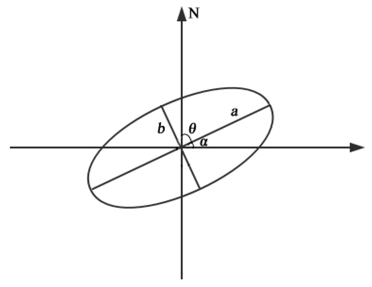
3.5. Directional Distribution Pattern and Migration Trend

Based on the comparison of the SDE parameters of the part I and part II under three RCPs, we studied the spatial distribution pattern of the C. deserticola in 2050s and 2070s. In 2050s, the SDEx, SDEy, and rotation angle increased gradually with the increase of RCP in part I (Table 3). This increasing trend indicated that the distribution of C. deserticola in the main direction and second direction will disperse gradually, the main direction of the distribution presents east–west pattern. The greater the ellipticity, the more dispersed the distribution. The ellipticity of part I was I21 (0.942) > I31 (0.941) > I21 (0.937) (Table 3), the distribution of C. deserticola was the most dispersed under RCP4.5 (Figure 8, I21). In part II, the ellipticity was II21 (0.968) > II11 (0.899) > II31 (0.757), the distribution of C. deserticola was more dispersed with increasing concentration path, and the main distribution direction presents northwest–southeast pattern (Figure 7a, II).
In 2070s, the main distribution direction of the two regions were same as those in 2050s, the ellipticity of part I and part II were as follow, I12 (0.958) > I32 (0.924) > I22 (0.904), and II12 (0.967) > II22 (0.909) > II32 (0.902) (Figure 7b). The distribution of C. deserticola was more centralized with increasing concentration path in part I. SDEx, SDEy, and rotation angle decreased gradually with the increase of RCPs in part II (Table 3). In general, the degree of concentration will intensify under the same RCP as time goes, which means that the future climate and environmental changes would easily lead to the habitat migration of C. deserticola.
The centroid was calculated by using the module of mean center in ArcGIS toolbox to get the longitude and latitude of under three RCPs, and the centroid migration route from the 2050s to 2070s was mapped (Figure 8). The results showed that geographical habitat of species is moving towards higher latitude during the process of climate warming, as global climate change has caused the temperature to rise, the temperature zone to move north, and precipitation to increase. Specifically, in part I, the overall centroid distribution of C. deserticola showed a trend of migration northward over time. The migration pathway angle under RCP2.6 and RCP8.5 was greater than 11.25°, showing a trend of northeast migration. The angle of migration pathway was greater than 90° under RCP4.5, with a tendency to the northwest (Figure 8a). As for part II, the angle of centroid migration pathway was less than 11.25° under RCP2.6, with a trend of eastward migration. With the increase of RCPs, the distribution of centroid gradually would move northwest (Figure 8b). Hence, our results were consistent with the previous studies [66,67].

4. Discussion

4.1. RF Model

At present, in the developed SDMs, simple algorithmic models such as GLM, CTA, and SRE have poor performance, and the simulation results will overestimate the potential area of species distribution. Complex machine learning models, such as RF, ANN, and MaxEnt, have better spatial distribution performance to some extent [68]. For example, MaxEnt is the most popular species distribution model in recent years because of its friendly data interface and simple data requirements. However, researchers did not change the default parameters in the process of MaxEnt modeling, so the model cannot satisfactorily meet the existing conditions of the model construction, which makes MaxEnt more sensitive to sampling deviation, and also has the problem of over-fitting [69]. While, among the SDMs, only the MaxEnt model can use categorical data as environmental variable inputs [10,54]. Therefore, soil variables and species point data were applied to MaxEnt to construct the restriction model in this paper. Regression ensemble of RF can describe the relationship between multiple independent variables (environmental factor) and a single dependent variable (species presence probability) [70]. Overall, RF combines regression and classification algorithms and takes multiple factors into account in the modeling. This unique working principle makes the error relatively low. Moreover, the model is based on multiple decision trees to fit a classification tree together, so it has become a machine learning method with good predictability and high frequency of use in most SDMs. Therefore, we choose the RF to construct prediction model based on machine learning.
Of course, it is essential for the modeler to avoid the selection of single model, or eliminate or reduce the bias caused by model selection, so that all models can participate in order to improve the advantage of ensembles of small models (ESMs) [71]. Nowadays, the ESMs have become a new trend and method to study species distribution [72,73]. After weighing several single models with high performance, the combination model is constructed. The suitable habitat distribution area of species obtained is very close to the actual results, which reduces the model uncertainty to a certain extent and has certain universality. Compared with single SDMs, the ESMs have some limitations [71]. The first drawback of the ESMs is its higher computational complexity and time consuming. The lack of implementation capabilities of current statistical software (such as R) also limits its use. In addition, ESMs are thought to be particularly useful when applied to rare species, the question is how rare a species must be to make ESMs outperform standard SDMs [74]. Although ESMs can be widely used in general species at present, for some species, many background points could be located far away from presence points, leading to high AUC values by easily distinguishing the background from presence points [75]. Therefore, after comparison and screening, we choose RF with the best prediction accuracy in a single model to run to reduce uncertainty. Meanwhile, we also have tried to explore the use of ESMs to study the evaluation and comparison of species distribution models [24].

4.2. Evaluation Indexes

According to the research results, three evaluation indexes—AUC, TSS, and KAPPA—were used to evaluate the RF model. The accuracy of the first two indicators was relatively high and close, while the accuracy of KAPPA was small, but on the whole, these three indicators all proved that the prediction accuracy of the RF model was very high (Figure 4). According to the difference of SDMs, the evaluation indexes of the model could be divided into threshold-dependent and threshold-independent. Specifically, AUC is a threshold independent evaluation metric and is considered to be a valid measure of the performance of an ordered scoring model [76]. However, the application of SDMs in conservation planning, such as identification of biodiversity hotspots and selection of representative conservation sites, often requires the presence–absence maps of species distribution [53]. In this case, the prediction accuracy should be evaluated based on the selected threshold-related indicators. KAPPA is one of the widely used model performance measurements for predicting accuracy the presence–absence maps, but it has serious limitations. Therefore, TSS is further proposed to compensate for the disadvantages while maintaining all the advantages of KAPPA, which is not affected by prevalence and verification set size. It provides a threshold-dependent evaluation measurement, which can be easily applied to presence–absence prediction, and its value is highly correlated with threshold-independent AUC statistics. The statistical values of TSS and AUC in this study are relatively close. This is consistent with other research results [53]. TSS can be used as an appropriate alternative to AUC when model predictions are expressed as presence–absence maps.
Besides, the results showed that the AUC and TSS statistical values of the evaluation indicators are relatively higher, which directly indicates that the model has excellent prediction performance, and may also indicate that the data or space have strong autocorrelation. There are many factors affecting the accuracy of prediction results in the modeling process, including the geographical scope of the study area, the natural distribution of species, and how the potential distribution of suitable habitats evolves as environmental conditions change. We have noticed that most scholars did not consider geographic location and spatial transmission in model accuracy assessment [77]. Therefore, if dispersal and biogeographic history are included, the results may differ. Consequently, the threshold range of the evaluation indexes in each model will vary, but this does not mean that any of the statistics are misleading [78]. In a word, the difference in model prediction performance is measured by different statistical data [79]. It should be determined according to the correlation between the appropriate statistical data and the application of the model, which cannot be generalized. Perhaps, some models have a higher AUC, TSS, but the performance difference between ‘known’ and ‘independent area’ climates is greater, while others have a lower AUC, TSS but performance is more stable in different climates [80].

4.3. Environment Variable and Scenarios

The factors affecting species distribution are multiple, such as climate, topography, soil, human activities, species interactions, and physiological characteristics of species, etc. [81,82,83]. Most of these data can be obtained and used. The factors involved in the model vary depending on the research species. In this study, bioclimatic factors were selected to model and predict the potential habitats distribution, and soil variables were used as limiting factors to further evaluate the comprehensive suitability distribution (Table 1). On the one hand, the research species are C. deserticola and H. ammodendron located in the arid area of Northwest China, and most of the land suitable for their growth was sandy land. The change rate of soil properties and topographic factors such as elevation of habitats is very delicate over a long-time scale from past to future, so it is feasible to predict future habitat distribution [84,85]. Global Human Influence Index (HII) can reflect the distribution form and state of the scope and intensity of human activities in geographic space. According to research results, the core potential distribution areas of C. deserticola were distributed in the Xinjiang Uygur Autonomous Region, the junction of Shaanxi–Gansu–Ningxia provinces, and the Inner Mongolia Autonomous Region (Figure 7), where the population distribution is sparse and the urban development is slow. These factors are not enough to affect the habitat of wild C. deserticola. On the other hand, from the time perspective, the time horizon and scale of existing land types and human activities data do not match the climate data. If we want to further analyze the impact of these factors, we must strive to solve the coincidence degree between the spatial and temporal resolution. Therefore, this paper only explored the impact of climate change and soil condition on the distribution of C. deserticola assuming that the topography and soil will not change in a short period of time.
In fact, the future climate scenarios were forecasted and evaluated by taking into account land use, population density, economic development, living and production mode, and other factors. The 19 bioclimatic factors selected in this paper are divided into two basic elements: temperature and precipitation, which play a leading role in the growth of C. deserticola. RCPs are common emission scenarios for predicting the suitable habitat distribution of species under future climate change [86,87]. It is predicted that by the end of the 21st century (2081–2100), from RCP2.6 to RCP4.5, and then to RCP 8.5, the global average surface temperature may increase by 0.3 °C–1.7 °C, 1.1 °C–2.6 °C, and 2.6 °C–4.8 °C, respectively [1], compared with the average temperature during 1986–2005. Therefore, the intensity of the emission scenario will prove to be a key factor determining the uncertainty level in future prediction [76]. The analysis of the threshold range of the main factors affecting the distribution of C. deserticola could determine the future trend of climate change and indirectly reflect the degree of adaptation of C. deserticola to climate change. We predicted that the spatial migration trend of C. deserticola would increase with the intensity of emission scenarios, so the prediction uncertainty would increase with time (Table 3). Therefore, neglecting the migration parameters may lead to errors when simulating higher emission scenarios or longer periods of time.

4.4. Parasitic and Host Plants

According to our prediction, the potential suitable habitats of parasitic plant C. deserticola and host plant H. ammodendron were roughly distributed in the desert and basin of the Xinjiang Uygur Autonomous Region, Qinghai province, the Inner Mongolia Autonomous Region, the Ningxia Hui Autonomous Region, Gansu province, and Shaanxi province (Figure S1). The habitat area of H. ammodendron was obviously larger than that of C. deserticola. By superimposing the suitable habitats of these two species, we could further concluded that the core potential suitable area for the growth of C. deserticola is located in the northwest of the Xinjiang Uygur Autonomous Region, the junction of Shaanxi–Gansu–Ningxia provinces, and the central of Inner Mongolia Autonomous Region (Figure 7). These areas were located in the northwest inland area of China. Affected by the cold winter air of Mongolia and Siberia and blocked by the surrounding mountains, the wet summer monsoon from the ocean is difficult to reach, which makes the habitats rare in precipitation and drought all year round. The growth environment of C. deserticola is very poor. It is predicted that with the passage of time and the enhancement of emission scenarios, the core potential distribution area of C. deserticola will decrease gradually. We should also highlight that suitability projections are only potential distributions based on climatic factors rather than future distribution predictions.
There are many factors affecting the reduction of suitable habitats of C. deserticola in the future, among which climate change is the main reason, and the external factors such as artificial digging could be ruled out. However, compared with these factors, the habitat decline of H. ammodendron will cause great damage to C. deserticola, which is the main threat to the habitat of C. deserticola. As the skin disappears, what will the hair stick to? As a parasitic plant, if the host disappears, C. deserticola naturally would not exist. H. ammodendron is a very important windbreak and sand fixation plant. The direct consequence of habitat degradation of H. ammodendron is desert expansion. In the case of preventing desert expansion, the protection of H. ammodendron in China is still effective, mainly reflected in a large number of artificial planting of H. ammodendron to prevent wind and fix sand, so the habitat of C. deserticola may also be correspondingly protected. Of course, this paper only studies the geographical distribution of C. deserticola and its host H. ammodendron, and further attempts should be made to analyze the interaction between the parasitic relationship, and habitat distribution of H. ammodendron and C. deserticola from the perspective of biomass and biological characteristics [88,89].

4.5. Protection of Desert Forest Ecosystem

Nowadays, global land desertification is becoming more and more serious. A large number of forests have been felled and cultivated, which has led to the gradual expansion of desertification areas in various countries, and the growing problems of environmental pollution especially in desert areas. In order to mitigate and solve the desertification, countries are vigorously preventing people from cutting down at will, supporting the conversion of farmland to forests and development of desert forest systems. Most land types of C. deserticola and H. ammodendron are sandy or semi-fixed dunes that are easily disturbed by natural and human factors. If the surface vegetation of these two species distribution areas was destroyed, the habitats will evolve into deserts. H. ammodendron is a native sand-fixing plant in desert area, it has strong characteristics of drought resistance, heat resistance, and cold resistance [39,40,90]. H. ammodendron, as an excellent tree species for sand fixation and afforestation in arid areas of Northwest China and desert areas of Inner Mongolia, plays a vital role in reducing soil erosion and protecting desert forest ecosystem. Consequently, the protection of H. ammodendron forest not only has the advantage of windbreak and sand fixation, but also actively promotes the growth of C. deserticola and protects the ecological benefits of endangered species.

5. Conclusions

This study analyzed the comprehensive habitat distribution of parasitic plant C. deserticola and its host plant H. ammodendron under future climate scenarios. The feasibility of using an RF model to predict potential geographical distribution is tested in this research. The results indicated that AUC and TSS were more stable for model evaluation and more accurate in forecasting.
The bioclimatic factors with greater impact on the distribution of C. deserticola are Bio6 (min temperature of coldest month/°C, Bio12 (annual precipitation/mm), Bio13 (precipitation of wettest month/mm), Bio16 (precipitation of wettest quarter/mm), and Bio18 (precipitation of warmest quarter/mm), respectively. The studies have shown that the sensitivity of C. deserticola on precipitation index is higher than the temperature index.
Potential highly suitable area of C. deserticola were distributed in 43° N–48° N, 80° E–89° E (part I) of arid and semi-arid area, and 39° N–42° N, 101° E–119° E (part II) of northwest temperate and warm temperate desert area. Moderately suitable areas were basically distributed in the peripheral extension areas of highly suitable, where the habitat range showed a decreasing trend. The scenarios with higher RCPs would have a larger impact on the spatial distribution pattern of species in the future. Since the impact of climate change on species produced is not reversible, it is necessary to strengthen the protection of C. deserticola.
According to the migration trend and the core potential suitable habitat distribution of C. deserticola, we should protect the ecosystems environment of distribution zones to expand habitats effectively. While protecting the habitat of C. deserticola from destruction, it is of great significance to improve the yield and quality of C. deserticola as the traditional Chinese medicine for sustainable development.

Supplementary Materials

The following are available online at https://www.mdpi.com/1999-4907/10/9/823/s1. Figure S1: Potential comprehensive habitat suitability of C. deserticola (a) and H. ammodendron (b) in current.

Author Contributions

J.L. and Y.Y. designed and performed the experiments, wrote the paper. J.L., Y.Y., Q.Z.Z., X.Z. (Xuhui Zhang), and X.Z. (Xiaoyan Zhang) collected and processed the experimental data. W.G. and H.Y.W. conceived and organized the paperwork, reviewed drafts, and improved the final manuscript.

Funding

This research is supported by the National Natural Science Foundation of China (no. 31070293), and the Research and Development Program of Science and Technology of Shaanxi Province (no. 2014-01-02).

Acknowledgments

We are grateful to each of the resource sharing platforms, such as GBIF, CVH, IPNI, WorldClim, and so on, which provide us with sampling data and climate data to be used in species distribution model. Also, we appreciate Yunfei Gu, a doctoral student at the University of Southampton for assisting us in revising the paper.

Conflicts of Interest

The authors declare that they have no competing interests.

References

  1. IPCC Climate Change. The Physical Science Basis. Contribution of Working Group I to the Fifth Assessment Report of the Intergovernmental Panel on Climate Change; Stocker, T.F., Qin, D., Plattner, G.K., Tignor, M., Allen, S.K., Boschung, J., Nauels, A., Xia, Y., Bex, V., Midgley, P.M., Eds.; Cambridge University Press: Cambridge, UK, 2013; p. 1535. [Google Scholar]
  2. Ding, Y.; Ren, G.; Shi, G.; Gong, P.; Zheng, X.; Zhai, P.; Zhang, D.; Zhao, Z.; Wang, S.; Wang, H.; et al. China’s national assessment report on climate change (I): Climate change in china and the future trend. Adv. Clim. Chang. Res. 2007, 3, 1–5. [Google Scholar]
  3. Guo, Y.; Wei, H.; Lu, C.; Gao, B.; Gu, W. Predictions of potential geographical distribution and quality of Schisandra sphenanthera under climate change. PeerJ 2016, 4, e2554. [Google Scholar] [CrossRef] [PubMed]
  4. Meynard, C.N.; Gay, P.E.; Lecoq, M.; Foucart, A.; Piou, C.; Chapuis, M.P. Climate-driven geographic distribution of the desert locust during recession periods: Subspecies’ niche differentiation and relative risks under scenarios of climate change. Glob. Chang. Biol. 2017, 23, 4739–4749. [Google Scholar] [CrossRef]
  5. Shabani, F.; Kumar, L.; Esmaeili, A.; Saremi, H. Climate change will lead to larger areas of Spain being conducive to date palm cultivation. J. Food Agric. Environ. 2013, 11, 2441–2446. [Google Scholar]
  6. Easterling, D.R.; Meehl, G.A.; Parmesan, C.; Changnon, S.A.; Karl, T.R.; Mearns, L.O. Climate extremes: Observations, modeling, and impacts. Science 2000, 289, 2068–2074. [Google Scholar] [CrossRef] [PubMed]
  7. Mccarty, J.P. Ecological consequences of recent climate change. Conserv. Biol. 2001, 15, 320–331. [Google Scholar] [CrossRef]
  8. Chapman, J.W.; Bell, J.R.; Burgin, L.E.; Reynolds, D.R.; Pettersson, L.B.; Hill, J.K.; Bonsallg, M.B.; Thomasg, J.A. Seasonal migration to high latitudes results in major reproductive benefits in an insect. Proc. Natl. Acad. Sci. USA 2012, 109, 14924–14929. [Google Scholar] [CrossRef] [Green Version]
  9. Gómez-Ruiz, E.P.; Lacher, T.E. Modelling the potential geographic distribution of an endangered pollination corridor in Mexico and the United States. Divers. Distrib. 2017, 23, 67–78. [Google Scholar] [CrossRef]
  10. Guo, Y.; Li, X.; Zhao, Z.; Wei, H.; Gao, B.; Wei, G. Prediction of the potential geographic distribution of the ectomycorrhizal mushroom Tricholoma matsutake under multiple climate change scenarios. Sci. Rep. 2017, 7, 46221. [Google Scholar] [CrossRef]
  11. Tang, C.; Dong, Y.; Herrandomoraira, S.; Matsui, T.; Ohashi, H.; He, L.; Nakao, K.; Tanaka, N.; Tomita, M.; Li, X.; et al. Potential effects of climate change on geographic distribution of the Tertiary relict tree species Davidia involucrata in China. Sci. Rep. 2017, 7, 43822. [Google Scholar] [CrossRef]
  12. Chen, S.; Cunningham, A.A.; Wei, G.; Yang, J.; Liang, Z.; Wang, J.; Wu, M.; Yan, F.; Xiao, H.; Harrison, X.A.; et al. Determining threatened species distributions in the face of limited data: Spatial conservation prioritization for the Chinese giant salamander (Andrias davidianus). Ecol. Evol. 2018, 8, 3098–3108. [Google Scholar] [CrossRef] [PubMed]
  13. Vencurik, J.; Bosela, M.; Sedmáková, D.; Pittner, J.; Kucbel, S.; Jaloviar, P.; Parobeková, Z.; Saniga, M. Tree species diversity facilitates conservation efforts of european yew. Biodivers. Conserv. 2019, 28, 791–810. [Google Scholar] [CrossRef]
  14. Shabani, F.; Kumar, L.; Taylor, S. Climate change impacts on the future distribution of date palms: A modeling exercise using climex. PLoS ONE 2012, 7, e48021. [Google Scholar] [CrossRef] [PubMed]
  15. Reside, A.E.; Vanderwal, J.; Garnett, S.T.; Utt, A.S. Vulnerability of Australian tropical savanna birds to climate change. Austral Ecol. 2016, 41, 106–116. [Google Scholar] [CrossRef]
  16. Chen, Y.; Vasseur, L.; You, M. Potential distribution of the invasive loblolly pine mealybug, Oracella acuta (Hemiptera: Pseudococcidae), in Asia under future climate change scenarios. Clim. Chang. 2017, 141, 719–732. [Google Scholar] [CrossRef]
  17. Wu, X.; Dong, S.; Liu, S.; Su, X.; Han, Y.; Shi, J.; Zhang, Y.; Zhao, Z.; Sha, W.; Zhang, X.; et al. Predicting the shift of threatened ungulates’ habitats with climate change in Altun Mountain National Nature Reserve of the Northwestern Qinghai-Tibetan Plateau. Clim. Chang. 2017, 142, 331–344. [Google Scholar] [CrossRef]
  18. Yang, L.; Zhang, C.; Chen, M.; Li, J.; Yang, L.; Huo, Z.; Ahmad, S.; Luan, X. Long-term ecological data for conservation: Range change in the black-billed capercaillie (Tetrao urogalloides) in northeast China (1970s–2070s). Ecol. Evol. 2018, 8, 3862–3870. [Google Scholar] [CrossRef]
  19. Koo, K.; Park, S.; Seo, C. Effects of climate change on the climatic niches of warm-adapted evergreen plants: Expansion or contraction? Forests 2017, 8, 500. [Google Scholar] [CrossRef]
  20. Wang, L.; Wang, W.; Wu, Z.; Du, H.; Zong, S.; Ma, S. Potential Distribution Shifts of Plant Species under Climate Change in Changbai Mountains, China. Forests 2019, 10, 498. [Google Scholar] [CrossRef]
  21. Keshtkar, H.; Voigt, W. Potential impacts of climate and landscape fragmentation changes on plant distributions: Coupling multi-temporal satellite imagery with GIS-based cellular automata model. Ecol. Inform. 2016, 32, 145–155. [Google Scholar] [CrossRef]
  22. Thodsen, H.; Baattrup-Pedersen, A.; Andersen, H.E.; Jensen, K.M.; Andersen, P.M.; Bolding, K.; Ovesen, N. Climate change effects on lowland stream flood regimes and riparian rich fen vegetation communities in Denmark. Int. Assoc. Sci. Hydrol. Bull. 2016, 61, 344–358. [Google Scholar] [CrossRef]
  23. Zhao, Z.; Guo, Y.; Wei, H.; Ran, Q.; Gu, W. Predictions of the potential geographical distribution and quality of a Gynostemma pentaphyllum base on the fuzzy matter element model in China. Sustainability 2017, 9, 1114. [Google Scholar] [CrossRef]
  24. Zhao, Z. Model construction and comparison of Species Distribution Models under climate change: A Case Study of Notopterygium incisum Ting Ex H. T. Chang. Master’s Thesis, Shaanxi Normal University, Xi’an, China, 2018. [Google Scholar]
  25. Aguilar-Soto, V.; Melgoza-Castillo, A.; Villarreal-Guerrero, F.; Wehenkel, C.; Pinedo-Alvares, C. Modeling the potential distribution of Picea chihuahuana Martínez, an endangered species at the Sierra Madre Occidental, Mexico. Forests 2015, 6, 692–707. [Google Scholar] [CrossRef]
  26. Alamgir, M.; Mukul, S.A.; Turton, S.M. Modelling spatial distribution of critically endangered Asian elephant and Hoolock gibbon in Bangladesh forest ecosystems under a changing climate. Appl. Geogr. 2015, 60, 10–19. [Google Scholar] [CrossRef]
  27. Brambilla, M.; Caprio, E.; Assandri, G.; Scridel, D.; Bassi, E.; Bionda, R.; Celada, C.; Falco, R.; Bogliani, G.; Pedrini, P.; et al. A spatially explicit definition of conservation priorities according to population resistance and resilience, species importance and level of threat in a changing climate. Divers. Distrib. 2017, 23, 1–12. [Google Scholar] [CrossRef]
  28. Ghaedi, M.; Ghaedi, A.M.; Negintaji, E.; Ansari, A.; Vafaei, A.; Rajabi, M. Random forest model for removal of bromophenol blue using activated carbon obtained from Astragalus bisulcatus tree. J. Ind. Eng. Chem. 2014, 20, 1793–1803. [Google Scholar] [CrossRef]
  29. Shruthi, R.B.; Kerle, N.; Jetten, V.; Stein, A. Object-based gully system prediction from medium resolution imagery using Random Forests. Geomorphology 2014, 216, 283–294. [Google Scholar] [CrossRef]
  30. Ma, Y.; Jiang, Q.; Meng, Z.; Li, Z.; Wang, D.; Liu, H. Classification of land use in farming area based on random forest algorithm. Trans. Chin. Soc. Agric. Mach. 2016, 47, 297–303. [Google Scholar]
  31. Peters, J.; Baets, B.D.; Verhoest, N.E.; Samson, R.; Degroeve, S.; Becker, P.D. Huybrechts W. Random forests as a tool for ecohydrological distribution modelling. Ecol. Model. 2007, 207, 304–318. [Google Scholar] [CrossRef]
  32. Evans, J.S.; Murphy, M.A.; Holden, Z.A.; Cushman, S.A. Modeling species distribution and change using random forest. In Predictive Species and Habitat Modeling in Landscape Ecology; Drew, C.A., Ed.; Springer: Berlin/Heidelberg, Germany, 2011; pp. 139–159. [Google Scholar]
  33. Bradter, U.; Kunin, W.E.; Altringham, J.D.; Thom, T.J.; Benton, T.G. Identifying appropriate spatial scales of predictors in species distribution models with the random forest algorithm. Methods Ecol. Evol. 2013, 4, 167–174. [Google Scholar] [CrossRef]
  34. Gama, M.; Crespo, D.; Dolbeth, M.; Anastácio, P. Predicting global habitat suitability for Corbicula fluminea using species distribution models: The importance of different environmental datasets. Ecol. Model. 2016, 319, 163–169. [Google Scholar] [CrossRef]
  35. Pliscoff, P.; Luebert, F.; Hilger, H.H.; Guisan, A. Effects of alternative sets of climatic predictors on species distribution models and associated estimates of extinction risk: A test with plants in an arid environment. Ecol. Model. 2014, 288, 166–177. [Google Scholar] [CrossRef]
  36. Wang, T.; Zhang, X.; Xie, W. Cistanche deserticola Y. C. Ma, “Desert Ginseng”: A review. Am. J. Chin. Med. 2012, 40, 1123–1141. [Google Scholar] [CrossRef] [PubMed]
  37. Cai, R.L.; Yang, M.H.; Shi, Y.; Chen, J.; Li, Y.C.; Qi, Y. Antifatigue activity of phenylethanoid-rich extract from Cistanche deserticola. Phytother. Res. 2010, 24, 313–315. [Google Scholar] [CrossRef]
  38. Jin, G.C.; Moon, M.; Jeong, H.U.; Min, C.K.; Sun, Y.K.; Oh, M.S. Cistanches Herba enhances learning and memory by inducing nerve growth factor. Behav. Brain Res. 2011, 216, 652–658. [Google Scholar]
  39. Shamsutdinov, Z.S.; Ubaidullaev, S.R. Distribution of Poa bulbosa L. and Carex pachystylis Gay within the phytogenous field of black saxaul. Probl. Desert Dev. 1988, 1, 38–43. [Google Scholar]
  40. Tobe, K.; Li, X.; Omasa, K. Effects of sodium chloride on seed germination and growth of two Chinese desert shrubs, Haloxylon ammodendron and H. persicum (Chenopodiaceae). Aust. J. Bot. 2000, 48, 455–460. [Google Scholar] [CrossRef]
  41. Xu, G.Q.; Li, Y.; Zou, T. Hydraulic resistance partitioning between shoot and root system and plant water status of Haloxyolon ammodendron growing at sites of contrasting soil texture. J. Arid Land 2010, 2, 98–106. [Google Scholar] [CrossRef]
  42. Naran, R.; Ebringerova, A.; HromàdkovÁ, Z.; PatoprstÝ, V. Carbohydrate polymers from underground parts of Cistanche deserticola. Phytochemistry 1995, 40, 709–715. [Google Scholar] [CrossRef]
  43. Zheng, G.; Song, Y.; Guo, S.; Ma, H.; Niu, D. Soluble sugar accumulation and the activities of sugar metabolism related enzymes in Cistanche deserticola and its host Haloxylon ammodendron. Acta Bot. Boreal Occident. Sin. 2006, 26, 1175–1182. [Google Scholar]
  44. Tan, D.; Guo, Q.; Liu, Y.; Ma, C.; Wang, X. The physiological metabolism reaction of Haloxylon parasitized by Cistanche deserticola. For. Res. 2007, 20, 495–499. [Google Scholar]
  45. Tu, P.; Jiang, Y.; Guo, Y. Review on the research progress and industry development of cistanches herba. J. Chin. Pharm. Sci. 2011, 46, 882–887. [Google Scholar]
  46. Thuiller, W.; Lafourcade, B.; Engler, R.; Araujo, M.B. BIOMOD: A platform for ensemble forecasting of species distributions. Ecography 2009, 32, 369–373. [Google Scholar] [CrossRef]
  47. Booth, T.H.; Nix, H.A.; Busby, J.R.; Hutchinson, M.F. BIOCLIM: The first species distribution modelling package, its early applications and relevance to most current MAXENT studies. Divers. Distrib. 2014, 20, 1–9. [Google Scholar] [CrossRef]
  48. Breiman, L. Bagging predictors. Mach. Learn. 1996, 24, 123–140. [Google Scholar] [CrossRef] [Green Version]
  49. Guisan, A.; Thuiller, W.; Zimmermann, N.E. Habitat Suitability and Distribution Models with Applications in R; Cambridge University Press: Cambridge, UK, 2017; p. 203. [Google Scholar]
  50. Friedman, J.H. Greedy function approximation: A gradient boosting machine. Ann. Stat. 2001, 29, 1189–1232. [Google Scholar] [CrossRef]
  51. Wang, Y.; Xie, B.; Wan, F.; Xiao, Q.; Dai, L. Application of ROC curve analysis in evaluating the performance of alien species’ potential distribution models. Biodivers. Sci. 2007, 15, 365–372. [Google Scholar]
  52. Kwon, Y.S.; Bae, M.J.; Hwang, S.J.; Kim, S.H.; Park, Y.S. Predicting potential impacts of climate change on freshwater fish in Korea. Ecol. Inform. 2015, 29, 156–165. [Google Scholar] [CrossRef]
  53. Allouche, O.; Tsoar, A.; Kadmon, R. Assessing the accuracy of species distribution models: Prevalence, kappa and the true skill statistic (TSS). J. Appl. Ecol. 2006, 43, 1223–1232. [Google Scholar] [CrossRef]
  54. Guo, Y.; Li, X.; Zhao, Z.; Nawaz, Z. Predicting the impacts of climate change, soils and vegetation types on the geographic distribution of Polyporus umbellatus in China. Sci. Total Environ. 2019, 948, 1–11. [Google Scholar] [CrossRef]
  55. Lefever, D.W. Measuring geographic concentration by means of the standard deviational ellipse. Am. J. Sociol. 1926, 32, 88–94. [Google Scholar] [CrossRef]
  56. Gong, J.X. Clarifying the standard deviational ellipse. Geogr. Anal. 2002, 34, 155–167. [Google Scholar] [CrossRef]
  57. Rahmaniati, M.; Eryando, T.; Susanna, D.; Pratiwi, D.; Nugraha, F.; Ruliansah, A.; Riandi, M.U. The utilization of standard deviational ellipse (SDE) model for the analysis of dengue fever cases in Banjar city 2013. Aspirator 2014, 6, 21–28. [Google Scholar] [CrossRef]
  58. Tang, J.; Ma, M.; Liu, L. Study on temporal and spatial evolution of structure of lodging industry and Influencing Factors in Red Tourism City—A case on Xiangtan City. J. Hunan Univ. Financ. Econ. 2018, 34, 72–80. [Google Scholar]
  59. Mitchell, A. The ESRI Guide to GIS Analysis, Volume 2: Spatial Measurements and Statistics; Esri Guide to GIS Analysis; ESRI Press: Redlands, CA, USA, 2005. [Google Scholar]
  60. Fischer, M.M.; Getis, A. Handbook of Applied Spatial Analysis: Software Tools, Methods and Applications; Springer: Berlin/Heidelberg, Germany, 2011. [Google Scholar]
  61. Yang, H.; Yan, B.; Qi, C.; Chen, D. Evaluation and analysis of wind resources in Jin-Jing-Ji region of China. Procedia 2011, 11, 836–842. [Google Scholar]
  62. Pishgar-Komleh, S.H.; Keyhani, A.; Sefeedpari, P. Wind speed and power density analysis based on Weibull and Rayleigh distributions (a case study: Firouzkooh county of Iran). Renew. Sustain Energy Rev. 2015, 42, 313–322. [Google Scholar] [CrossRef]
  63. Chen, J.; Xie, C.; Chen, S.; Sun, C.; Zhao, R.; Xu, R. Suitability evaluation of Cistanche desertiola based on TCMGIS-I. China J. Chin. Mater. Med. 2007, 32, 1396–1401. [Google Scholar]
  64. Huang, X.; Xu, R.; Chen, J.; Yu, J.; Liu, S.; Liu, T. Status and prospect of studies on habitat characteristics, parasitic mechanism and nutrient transport of Cistanche deserticola. China J. Chin. Mater. Med. 2012, 37, 2831–2835. [Google Scholar]
  65. Ma, S.; Wei, B.; Li, X.; Luo, C.; Sun, F. The impacts of climate change on the potential distribution of Haloxylon ammodendron. Chin. J. Ecol. 2017, 36, 1243–1250. [Google Scholar]
  66. Cheng, A.; Feng, Q.; Zhang, J.; Li, Z.; Wang, G. A Review of Climate Change Scenario for Impacts Process Study. Sci. Geogr. Sin. 2015, 35, 84–90. [Google Scholar]
  67. Mullan, D.; Swindles, G.; Patterson, T.; Galloway, J.; Macumber, A.; Falck, H.; Crossley, L.; Chen, J.; Pisaric, M. Climate change and the long-term viability of the World’s busiest heavy haul ice road. Theor. Appl. Climatol. 2016, 129, 1089–1108. [Google Scholar] [CrossRef]
  68. Elith, J.; Kearney, M.; Phillips, S. The art of modelling range-shifting species. Methods Ecol. Evol. 2010, 1, 330–342. [Google Scholar] [CrossRef]
  69. Elith, J.; Phillips, S.J.; Hastie, T.; Dudík, M.; Chee, Y.E.; Yates, C.J. A statistical explanation of MaxEnt for ecologists. Divers. Distrib. 2011, 17, 43–57. [Google Scholar] [CrossRef]
  70. Breiman, L. Random forests. Mach. Learn. 2001, 45, 5–32. [Google Scholar] [CrossRef]
  71. Breiner, F.T.; Guisan, A.; Bergamini, A.; Nobis, M.P. Overcoming limitations of modelling rare species by using ensembles of small models. Methods Ecol. Evol. 2015, 6, 1210–1218. [Google Scholar] [CrossRef]
  72. Briscoe, N.J.; Elith, J.; Salguero-Gómez, R.; Lahoz-Monfort, J.J.; Camac, J.S.; Giljohann, K.M.; Holden, M.H.; Hradsky, B.A.; Kearney, M.R.; McMahon, S.M.; et al. Forecasting species range dynamics with process—Explicit models: Matching methods to applications. Ecol. Lett. 2019, 1–17. [Google Scholar] [CrossRef] [PubMed]
  73. Lin, C.; Chiu, C. The Relic Trochodendron aralioides Siebold & Zucc. (Trochodendraceae) in Taiwan: Ensemble distribution modeling and climate change impacts. Forests 2019, 10, 7. [Google Scholar]
  74. Lomba, A.; Pellissier, L.; Randin, C.F.; Vicente, J.; Moreira, F.; Honrado, J.; Guisan, A. Overcoming the rare species modelling paradox: A novel hierarchical framework applied to an Iberian endemic plant. Biol. Conserv. 2010, 143, 2647–2657. [Google Scholar] [CrossRef]
  75. VanDerWal, J.; Shoo, L.P.; Graham, C.; Williams, S.E. Selecting pseudo-absence data for presence-only distribution modeling: How far should you stray from what you know? Ecol. Model. 2009, 220, 589–594. [Google Scholar] [CrossRef]
  76. McPherson, J.; Jetz, W.; Rogers, D. The effects of species’ range sizes on the accuracy of distribution models: Ecological phenomenon or statistical artefact? J. Appl. Ecol. 2004, 41, 811–823. [Google Scholar] [CrossRef]
  77. Engler, R.; Guisan, A. MigClim: Predicting plant distribution and dispersal in a changing climate. Divers. Distrib. 2009, 15, 590–601. [Google Scholar] [CrossRef]
  78. Lobo, J.M.; Jimenez-Valverde, A.; Real, R. AUC: A misleading measure of the performance of predictive distribution models. Glob. Ecol. Biogeogr. 2008, 17, 145–151. [Google Scholar] [CrossRef]
  79. Swets, J.A. Measuring the accuracy of diagnostic systems. Science 1988, 240, 1285–1293. [Google Scholar] [CrossRef]
  80. Shabani, F.; Kumar, L.; Ahmadi, M. A comparison of absolute performance of different correlative and mechanistic species distribution models in an independent area. Ecol. Evol. 2016, 6, 5973–5986. [Google Scholar] [CrossRef] [Green Version]
  81. Pearson, G.A.; Mota, L.L. Frayed at the edges: Selective pressure and adaptive response to abiotic stressors are mismatched in low diversity edge populations. J. Ecol. 2009, 97, 450–462. [Google Scholar] [CrossRef]
  82. Crowther, M.S.; Lunney, D.; Lemon, J.; Stalenberg, E.; Ellis, M. Climate-mediated habitat selection in an arboreal folivore. Ecography 2013, 36, 1–8. [Google Scholar] [CrossRef]
  83. Lee, D.S.; Bae, Y.S.; Byun, B.K.; Lee, S.; Park, J.K.; Park, Y.S. Occurrence prediction of the citrus flatid planthopper (Metcalfa pruinosa (Say, 1830)) in South Korea using a random forest model. Forests 2019, 10, 583. [Google Scholar] [CrossRef]
  84. Shabani, F.; Ahmadi, M.; Peters, K.J.; Haberle, S.; Champreux, A.; Saltréand, F.; Bradshaw, C.J.A. Climate-driven shifts in the distribution of koala-browse species from the Last Interglacial to the near future. Ecography 2019, 42, 1–13. [Google Scholar] [CrossRef]
  85. Booth, T.H. Impacts of climate change on eucalypt distributions in Australia: An examination of a recent study. Aust. For. 2017, 80, 208–215. [Google Scholar] [CrossRef]
  86. Xu, X.; Zhang, H.; Xie, T.; Xu, Y.; Zhao, L.; Tian, W. Effects of Climate Change on the Potentially Suitable Climatic Geographical Range of Liriodendron chinense. Forests 2017, 8, 399. [Google Scholar] [CrossRef]
  87. Adhikari, P.; Shin, M.S.; Jeon, J.Y.; Kim, H.W.; Hong, S.; Seo, C. Potential impact of climate change on the species richness of subalpine plant species in the mountain national parks of south korea. J. Ecol. Environ. 2018, 42, 36. [Google Scholar] [CrossRef]
  88. Tan, D.; Guo, Q.; Wang, C.; Ma, C. Effects of the parasite plant (Cistanche deserticola) on growth and biomass of the host plant (Haloxylon ammodendron). For. Res. 2004, 17, 472–478. [Google Scholar]
  89. Li, L.I.; Xu, X.; Sun, Y.; Han, W. Effects of parasitic plant Cistanche deserticola on chlorophyll a fluorescence and nutrient accumulation of host plant Haloxylon ammodendron in the Taklimakan Desert. J. Arid Land 2012, 4, 342–348. [Google Scholar] [CrossRef]
  90. Zou, X.; Wang, S. Strengthening the protection of desert forest resources—Haloxylon ammodendron. J. Inn. Mong. For. 2004, 6, 19. [Google Scholar]
Figure 1. Methodological approaches of comprehensive habitat suitability evaluation.
Forests 10 00823 g001
Figure 2. Geographic locations of C. deserticola and H. ammodendron, the black dots are the sampling points of C. deserticola, and the triangles are H. ammodendron. (I) study area; (II) study area in China. The red letters represent the counties and topographical units involved in study area. (a) Tacheng City; (b) Junggar Basin; (c) Hoboksar; Tacheng City; (d) Alashankou city; (e) Wusu city; (f) Shawan county; (g) Wenquan County; (h) Huocheng County; (i) Tianshan Mountains; (j) Badain Jaran Desert; (k) Alxa League; (l) Tengger Desert; (m) Hetao Plain; (n) Ningxia Plain; (o) Bayan Nur; (p) Baotou city; (q) Ordos city; (r) Mu Us Desert; (s) Hexi Corridor.
Forests 10 00823 g002
Figure 3. The schematic diagram and parameters of the standard deviation ellipse. N is the north direction, a and b is the major axis semidiameter and the minor axis semidiameter, θ is the rotation angle, and α is used to judge the distribution pattern.
Forests 10 00823 g003
Figure 4. Evaluation of prediction model under different RCPs in 2050s (a), and 2070s (b).
Forests 10 00823 g004
Figure 5. Comprehensive habitat suitability of C. deserticola under different RCPs in 2050s (a), and 2070s (b).
Forests 10 00823 g005
Figure 6. Comprehensive habitat suitability of H. ammodendron under different RCPs in 2050s (a), and 2070s (b).
Forests 10 00823 g006
Figure 7. The core potential geographical distribution of C. deserticola under different RCPs in 2050s (a), and 2070s (b).
Forests 10 00823 g007
Figure 8. Migration pathway of C. deserticola under the RCPs from 2050s to 2070s in part I (a) and part II (b).
Forests 10 00823 g008
Table 1. Environmental variables used for predicting potential distribution of C. deserticola and H. ammodendron.
Environmental VariablesVariableLabel
Bioclimatic VariablesAnnual Mean TemperatureBio1
Mean Diurnal Range (Mean of monthly (max temp − min temp))Bio2
Min Temperature of Coldest MonthBio6
Temperature Annual Range (Bio5-Bio6)Bio7
Mean Temperature of Driest QuarterBio9
Mean Temperature of Warmest QuarterBio10
Annual PrecipitationBio12
Precipitation of Wettest MonthBio13
Precipitation of Wettest QuarterBio16
Precipitation of Warmest QuarterBio18
Soil VariablesTopsoil USDA texture classificationT_USDA
Topsoil pH (H2O)T_PH
Topsoil Organic Carbon (% weight)T_OC
Topsoil Calcium Carbonate (% weight)T_CACO3
Topsoil Gypsum (% weight)T_CASO4
Subsoil pH (H2O)S_PH
Subsoil Organic Carbon (% weight)S-OC
Soil Type VariablesST
Table 2. Evaluation indexes and evaluation grades of the model.
EvaluationEvaluation Grade
IndexesBestBetterModerateGeneralFailed
AUC1.0–0.910.90–0.810.80–0.710.70–0.61<0.60
KAPPA1.0–0.810.80–0.610.60–0.410.40–0.21<0.20
TSS1.0–0.860.85–0.710.70–0.560.55–0.41<0.40
Table 3. The standard deviational ellipse’s parameters of the core potential distribution area of C. deserticola.
TimeRCPsResearchMean Center (°)SDE
x(km)
SDE
y(km)
Rotation θ
(°)
Ellipticity
PeriodArea X ¯ Y ¯
2050sRCP2.6I1184.19342.927528.040185.03278.8210.937
II11105.90839.740483.449212.16891.7250.899
RCP4.5I2185.77143.874662.348222.27380.3910.942
II21105.80240.5381707.532430.20096.5850.968
RCP8.5I3186.33243.613730.405246.19781.7750.941
II31105.07639.425371.492242.91399.1970.757
2070sRCP2.6I1287.00543.929726.342207.77785.1090.958
II12105.03240.311565.755144.64895.8940.967
RCP4.5I2285.47443.911613.714262.11379.4000.904
II22106.47140.401432.174180.05590.5260.909
RCP8.5I3286.50343.916634.586242.00282.2520.924
II32106.84539.712522.806225.79692.1480.902

