Article

Mobile Terrestrial Photogrammetry for Street Tree Mapping and Measurements

1
Orange County Extension, IFAS, University of Florida, 6021 South Conway Road, Orlando, FL 32812, USA
2
Department of Environmental Horticulture, CLCE, IFAS, University of Florida-Gulf Coast Research and Education Center, 14625 County Road 672, Wimauma, FL 33598, USA
3
Department of Geomatics, IFAS, University of Florida-Gulf Coast Research and Education Center, 1200 North Park Road, Plant City, FL 33563, USA
4
Department of Geomatics, IFAS, University of Florida, P.O. Box 110565, Gainesville, FL 32611-0565, USA
5
Department of Environmental Horticulture, CLCE, IFAS, University of Florida, P.O. Box 110670, Gainesville, FL 32611-0670, USA
6
School of Geosciences, University of South Florida, 4202 East Fowler Avenue, Tampa, FL 33620, USA
*
Author to whom correspondence should be addressed.
Forests 2019, 10(8), 701; https://doi.org/10.3390/f10080701
Submission received: 7 July 2019 / Revised: 31 July 2019 / Accepted: 7 August 2019 / Published: 19 August 2019

Abstract

:
Urban forests are often heavily populated by street trees along right-of-ways (ROW), and monitoring efforts can enhance municipal tree management. Terrestrial photogrammetric techniques have been used to measure tree biometry, but have typically used images from various angles around individual trees or forest plots to capture the entire stem while also utilizing local coordinate systems (i.e., non-georeferenced data). We proposed the mobile collection of georeferenced imagery along 100 m sections of urban roadway to create photogrammetric point cloud datasets suitable for measuring stem diameters and attaining positional x and y coordinates of street trees. In a comparison between stationary and mobile photogrammetry, diameter measurements of urban street trees (N = 88) showed a slightly lower error (RMSE = 8.02%) relative to non-mobile stem measurements (RMSE = 10.37%). Tree Y-coordinates throughout urban sites for mobile photogrammetric data showed a lower standard deviation of 1.70 m relative to 2.38 m for a handheld GPS, which was similar for X-coordinates where photogrammetry and handheld GPS coordinates showed standard deviations of 1.59 m and the handheld GPS 2.36 m, respectively—suggesting higher precision for the mobile photogrammetric models. The mobile photogrammetric system used in this study to create georeferenced models for measuring stem diameters and mapping tree positions can also be potentially expanded for more wide-scale applications related to tree inventory and monitoring of roadside infrastructure.

1. Introduction

Municipal forest management occurs at various scales throughout the urban landscape, but it often includes the direct management of individual trees. While conventional forestry is generally focused on increasing production at the stand level, urban forestry is more concerned with maximizing public forest benefits (e.g., aesthetics, shade, and property value) and minimizing tree-related risks. More recently, urban forest management practices have been placing a greater emphasis on the value of urban forests as related to their associated ecosystem services [1,2]. While models have been created to place a monetary value on the ecosystem services offered by urban forests [3], municipal management efforts are still largely shaped by a desire to limit property damage and operation expenses [4,5]. As such, urban forest managers often focus their management efforts on roadside planting areas, sites where trees may require increased levels of care to become established and grow [6,7]. This management often includes the collection of street tree inventory data as a means of establishing a baseline for future monitoring and assessment [8].
The tree and site conditions monitored in a tree inventory can vary greatly among municipalities based on management objectives. However, tree species, vitality, risk rating, geographic location (i.e., coordinates), and diameter at breast height (DBH) were shown by Östberg et al. [9] to be the most common inventory parameters by researchers, city officials, and arborists that work within urban forestry. More detailed data collection for these parameters comes at the price of increased labor, and there is always a trade-off between allocating resources toward conducting inventories and other management efforts that could benefit from inventory data (e.g., planting, pruning, and removal). Limited municipal resources can limit inventory efforts leading to many municipalities foregoing street tree inventories altogether [10,11].
Recent integration and advances in the accessibility of geospatial techniques, monitoring strategies, remote sensing, and geographic information systems (GIS) have led to new and more cost-effective monitoring strategies in urban forestry [12]. Coordinates for individual trees have become increasingly integral to urban tree inventories with the availability of global navigation satellite systems (GNSS), such as the US Global Positioning System (GPS); allowing for an easier transfer to GIS programs and integration with complementary datasets [8]. Urban tree canopy (UTC) cover, transportation and infrastructure, and property boundaries can be interpreted and measured together [13,14,15]. Techniques utilizing remotely-sensed aerial and satellite data have worked well to characterize UTC and prioritize tree planting efforts [16,17]. At the same time, terrestrial remote sensing techniques have even been utilized by non-professional volunteers to attain urban forest inventory data [18]. Advanced data processing techniques for analyzing forest crowns have taken advantage of high-resolution imagery [19], hyperspectral imagery [20,21], three-dimensional scanned data [22,23,24], and combinations of these datasets [25,26,27] to identify individual trees and collect measurements (e.g., species identification, crown dimensions, leaf area index, etc.) [28].
Aerial remote sensing data has fundamentally changed the analysis of urban forests, but traditional inventory methods are often still preferred for detailed data collection on individual trees (e.g., street trees) [1]. Nielsen et al. [29] noted that studies employing aerial and satellite data generally require ground-level field data for interpretation. Even with the integration of high-quality imagery and aerial laser scanning data, Tanhuanpää et al. [24] were only able to accurately identify 88.8% of all trees in an inventory along roadways. Similarly, Wu et al. [30] had a detection rate of 83.6% from a purely aerial laser scanning dataset. These results suggest that individual tree identification methods from aerial remote sensing are progressing, but have some room for improvement. Moreover, measurements like DBH, ground coordinates, and species identification from aerial laser scanning and aerial imagery still typically lack the accuracy and precision that can be attained from traditional field inventories conducted on the individual tree level [1,29,31].
Terrestrial remote sensing is less common but may be more applicable for managing individual trees. Terrestrial laser scanning utilizes light detection and ranging (LiDAR) to rapidly measure distances between a scanning unit and illuminated objects to create 3D representations of scanned areas. This technology has been utilized for many surveying applications to measure geologic features, ground surface, vegetation, archeological sites, and property planning for various types of infrastructure [32,33,34,35]. It has been adapted to accurately measure key forest inventory parameters (e.g., tree height, DBH, and leaf area index) [36]. In contrast with managed forest stands that serve as the backdrop for most existing research [36], urban environments are often compositionally more heterogeneous, and problems related to occlusion and poor scanning geometry tend to be more common. For example, Moskal and Zheng [37] showed urban terrestrial laser scanning point cloud measurements for DBH to be correlated (R2 = 0.68) with physical measurement, while Yao et al. [38] showed a range of correlations (R2 = 0.62−0.88) taken from a forest plot within a national park.
Additionally, terrestrial laser scanning data were collected from a stationary, tripod-mounted unit for many of the past studies [39] making data collection a time-intensive process [36]. Mobile laser scanning from a terrestrial perspective has allowed for datasets to be collected over large areas with survey-grade, centimeter-level accuracy under relatively short durations of time [40]. Holopainen et al. [41] showed that 79.22% of trees could be manually located in mobile laser scanning datasets with a root mean square error (RMSE) of 0.49 m when compared to terrestrial laser scanned datasets.
Applications of photogrammetry predate the use of LiDAR, but until recently, programs did not exist that could quickly produce photogrammetric models. However, this has changed with the development of inexpensive and commercially-available Structure-from-Motion (SfM) programs that use computer vision image-matching algorithms and user-interpreted ‘targets’ to generate three-dimensional photogrammetric models. These programs make it possible to create three-dimensional models with little more than a consumer-grade camera and a home desktop computer. Computer vision-assisted photogrammetry programs have been used from an aerial perspective to generate digital surface models (DSM) for applications in forestry and environmental monitoring [42,43]. Mapping with these models can be used to create estimates for tree height and other metrics of canopy cover [44].
More recently, ground-based, stationary photogrammetry has also been used to measure volume, height, diameter, and surface area for individual trees [45,46,47], trees positioned within forest plots [48,49,50,51,52], and root systems [53] (Table 1). Even when the photogrammetric process is conducted to create models of stems along roadways [54], the process for attaining model measurements is more intensive than traditional field measurements. Beyond this limitation, photogrammetric methods may have difficulty in assessing certain aboveground vegetation parameters (e.g., canopy width, tree height, etc.) due to shade, geometric limitations, and canopy occlusion; as Surový et al. [49] showed, stems modeled within a close-range photogrammetry program from a forest study plot showed a stem diameter RMSE of 0.59 cm, and noted error was associated with low visibility areas.
Close-range photogrammetry has the potential to become an efficient means of inventorying and measuring street trees while avoiding the high equipment costs associated with terrestrial laser scanning that range from tens of thousands to ~$/€100,000. While others have demonstrated the potential of using fixed cameras to capture the imagery needed to model trees, there are few if any studies that have looked at mobile SfM photogrammetry techniques to measure woody vegetation in urban environments. For this study, we compared the location and stem diameter measurements derived from both georeferenced mobile SfM photogrammetry and stationary SfM data. The results from both methods were then compared to field-derived DBH and location measurements. In conducting this study, we hoped to demonstrate the potential of mobile SfM photogrammetry to inventory street trees in urban conditions.

2. Materials and Methods

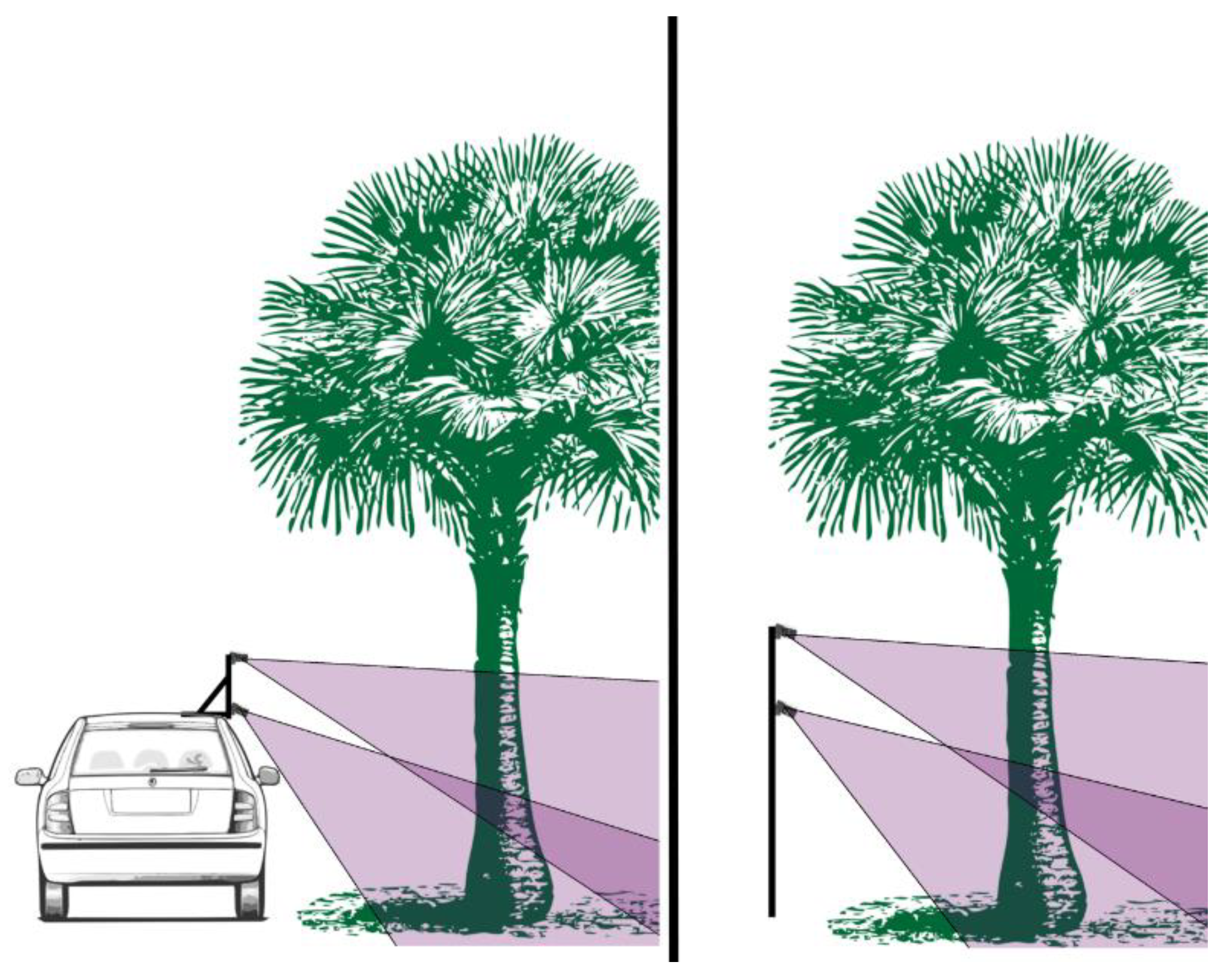
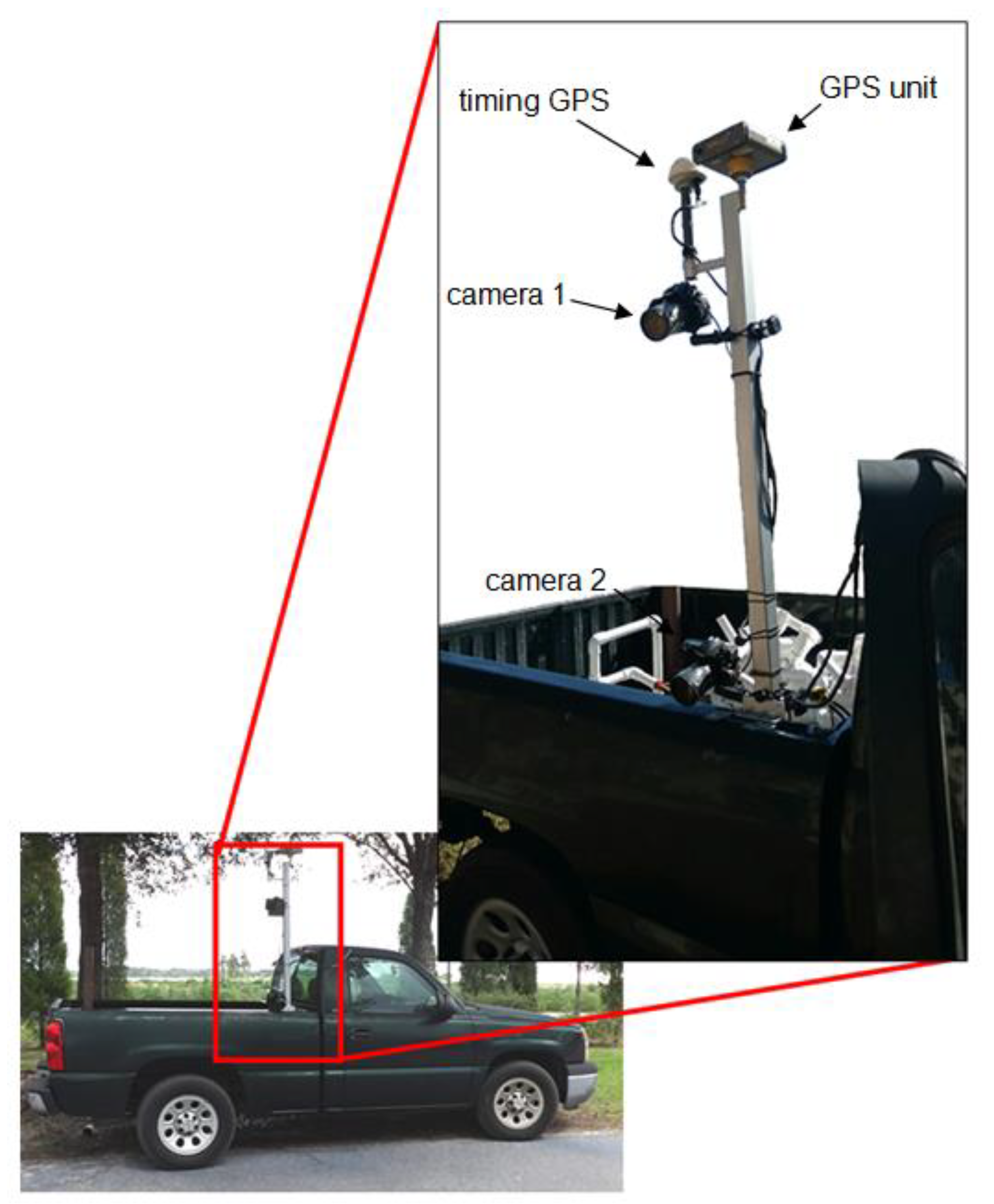
2.1. Study Site and Field Methods

Data were collected from ten sites along 100 m transects. One site was located along a windbreak composed of loblolly pine (Pinus taeda L.) trees (N = 52) at the University of Florida (UF) Gulf Coast Research and Education Center in Wimauma, FL (~27°45′40″ N and ~82°13′40″ W). The remaining nine sites were randomly selected 100 m sections of right-of-way along designated hurricane priority routes within Tampa, FL (27°57′50.97″ N, 82°27′9.38″ W). The windbreak site provided relatively uniform conditions to test the photogrammetric set-up (e.g., non-occluded stems, relatively circular pine stems, uniform light conditions, etc.), while the urban sites represented a greater range of challenges to the set-up and post-processing. The spacing of urban stems was sparser along urban right-of-ways, requiring more study area to test the proposed set-up under a variety of heterogeneous urban conditions and achieve a comparable sample size. The street trees (N = 88) representing the urban sites included Quercus virginiana Mill. (31.5%), Quercus laurifolia Michx. (27.0%), Washingtonia robusta H.Wendl. (11.2%), Ulmus parvifolia Jacq. (7.9%), Acer rubrum L. (4.5%), Sabal palmetto (Walt.) Lodd. (4.5%), Prunus caroliniana (Mill.) Aiton (4.5%), Pinus elliottii Engelm. (3.4), Syagrus romanzoffiana (Cham.) Glassman (3.4%), Quercus laevis Walter (1.1%), and Dalbergia sissoo Roxb. (1.1%). Stem DBH measurements were collected with a DBH tape as a control. Control measurements for stem position were visually interpreted from very high resolution (i.e., 0.65 m) orthoimages originally captured from the QuickBird satellite (DigitalGlobe, Inc., Longmont, CO, USA). However, some stems were occluded by canopy, so objects (e.g., street signs, light poles, fire hydrants, transformer boxes, etc.) or conspicuous ground features (e.g., sidewalk cracks, road markers, etc.) in the field were used as ‘anchor points’ to measure compass heading direction and distance with a laser rangefinder (TruPulse 200—Laser Technology Inc., Centennial, CO, USA). These measurements could then be used to approximate the occluded stem position from the visible ‘anchor point’ within a GIS (specifically, Google Earth) using the ruler tool to interpret heading and distance. An additional set of coordinates were measured with a handheld GPS unit with a circular error probability of 1–1.5 m (GNSS Surveyor—Bad Elf, LLC, Tariffville, CT, USA) to also include geospatial positional measurements often taken during standard tree inventories as a comparison.
Imagery for photogrammetric data was collected with two stereoscopic camera set-ups. The stationary camera set-up used a surveying rod to secure a digital single-lens reflex (DSLR) camera (Canon EOS Rebel T3—Canon Inc., Tokyo, Japan). Two passes along the transect were made to ensure high overlap between different tree positions—a pass with the camera mounted on a surveying rod at 1.6 m and tilted downward at a −25° angle, and another at 2.0 m at a −30° angle. In this manner, data collection simulated a two camera photogrammetric set-up (Figure 1). Images were captured at ~0.33 m intervals along each transect pass. Similarly, the mobile photogrammetric set-up utilized a two DSLR camera (Nikon D300—Nikon Co., Tokyo, Japan) system for image capture along the sampled right-of-ways (ROW; i.e., publicly-managed corridor) areas. The mobile set-up was similar to the system used by Abd-Elrahman et al. [55] and Abd-Elrahman et al. [56], where a second DSLR camera was used to replace the hyperspectral camera used in the original system. The mobile images were collected in concert with a similarly-positioned survey-grade (i.e., centimeter-level) GPS unit (Hyperlite+, Topcon Corp., Tokyo, Japan) and a timing GPS antennae (Accutime Gold™, Trimble Navigation Ltd., Sunnyvale, CA, USA), in order to retroactively assign coordinate metadata to each image in post-processing (Figure 2). Similar to the stationary set-up, the cameras were positioned at 1.6 m and tilted downward at a −25° angle and 2.0 m at a −30° angle. Mobile images were also captured along straight sections of road moving in the direction of traffic at every ~0.33 m for adequate image overlap, which required the vehicle to travel at ~10 km/h over 3 separate passes with the utilized camera settings. High overlap (Equation (1)) is needed for photogrammetric camera positioning.
Overlap = (G − B)/G
where B is the distance between photos (i.e., orthogonal to the direction that the camera is aimed) and G is photo coverage in the direction of camera movement. Photos were taken at ~0.33 m intervals, hence, photos ranged between 83 and 96% overlap based on the distances of trees from the roadway camera position, ranging from 2 m to 8.5 m, respectively.

2.2. Model Processing and Measurements

All datasets were processed with close-range, photogrammetry software, (Photoscan Professional, AgiSoft LLC, St., Petersburg, Russia) to generate 3D models. Mobile datasets utilized kinematic GPS data post processing to assign image positions based on synchronized timing from camera metadata and GPS (Figure 2). The resulting point clouds were already georeferenced and suitable for use within supporting GIS programs. Stationary datasets were not georeferenced, but the scale was established via a measuring ruler with control point marks of known distance. The mobile imagery utilized the coordinates taken from the geodetic grade GPS receiver, which allowed the position of each photo location to be set, and photogrammetrically aligned, prior to point cloud generation. Vertical sections of the stems were excised from the point clouds via hand measurement at approximately 1.4 m above the ground with the “point selection” tool in CloudCompare. The “point selection tool” was then also used to manually measure diameter from stem sections with the “point selection” tool by measuring the distance of points representing one side of the stem to points along the opposite side.

2.3. Data Analysis

All data were analyzed in the Microsoft Excel [57]. Similar to previous publications that assessed the accuracy of modeled vegetation, root mean square error (RMSE) (Equation (2)) and bias (Equation (3)) were used to test model accuracy of DBH [46].
RMSE   =   i = 1 n ( y i y i ) ^ 2 n
Bias   =   i = 1 n ( y i y i ^ ) n
These equations were executed with the number of estimates (n), the value estimated by the models ( y i ), and the physical measurement ( y i ^ ). A linear regression analysis was also used to compare DBH measurements derived from close-range photogrammetry to their physical measurements with the lm() function in R (www.r-project.org).

3. Results

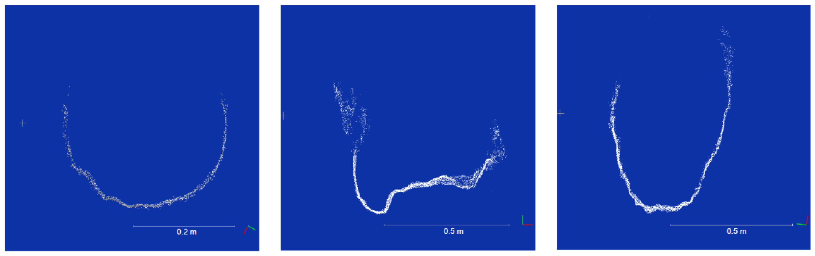
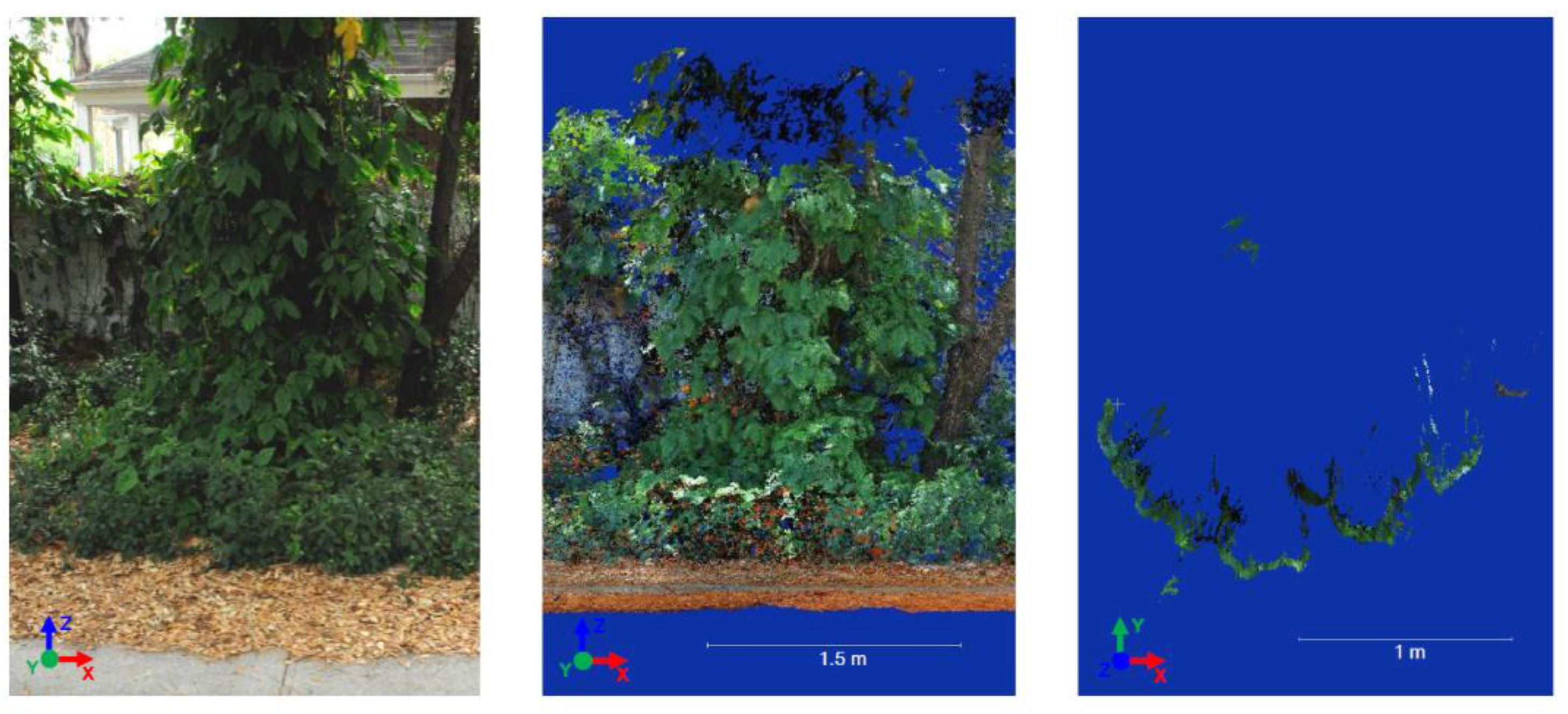
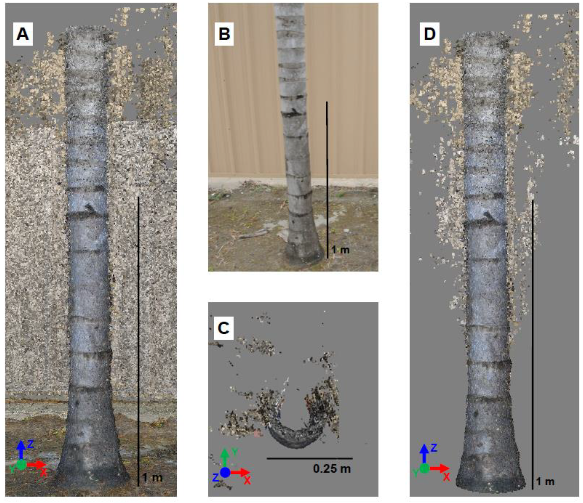
3.1. General Site and Point Cloud Observations

Stems from urban sites showed greater diversity in size relative to the windbreak site, as the average DBH was 27.1 cm with a range of 59.7 cm (min. = 4.6 cm, max. = 64.3 cm). There were 52 stems from the windbreak site of one species (Pinus taeda L.), and were likely from a single relatively recent planting event; so overall DBH size (mean = 14.2 cm) and variation (min. = 5.6 cm, max. = 22.9 cm) were lower than the sampled urban trees.
All trees sampled along the right-of-way were relatively close to the roadway, ranging approximately from two to seven meters from the camera when being directly photographed. As trees closest to the camera are expected to have greater pixel densities, the associated point clouds typically show similar distance decay. For the closest tree (1.6 m from the roadway), the side of a pixel (i.e., ground sample distance) was 0.09 cm and the point density of 44.5 points from a 1 cm stem slice taken at 1.4 m. Alternatively, the furthest tree (8.5 m from the roadway) had a side of a pixel (i.e., ground sample distance) of 0.24 cm and the point density of 19.8 points from a 1 cm stem slice taken at 1.4 m.

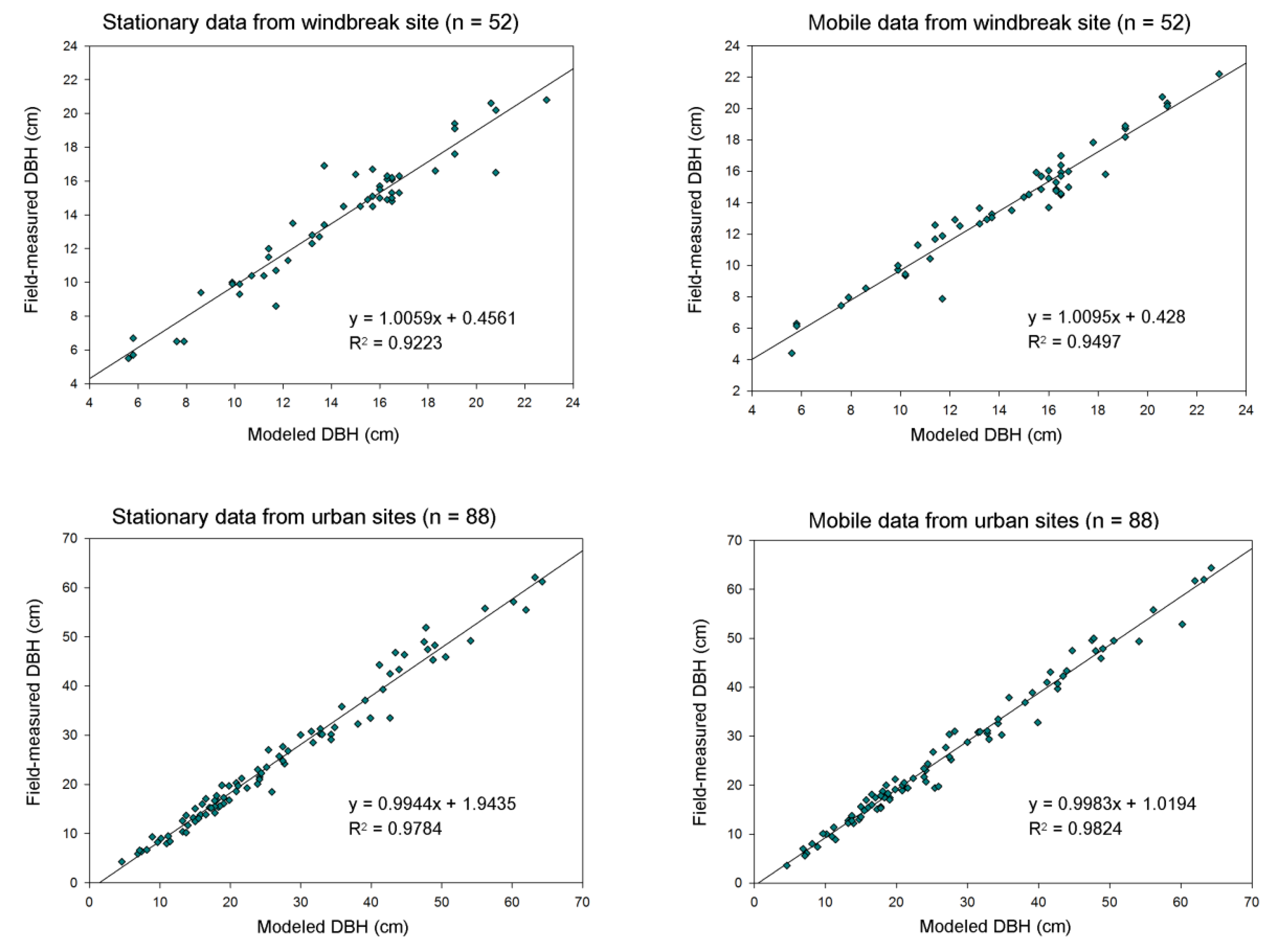
3.2. Mobile vs. Stationary
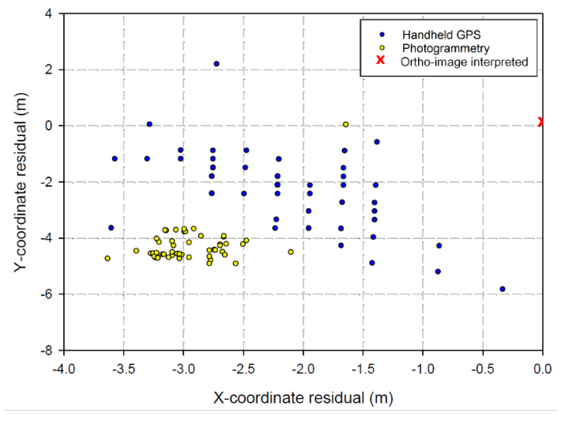
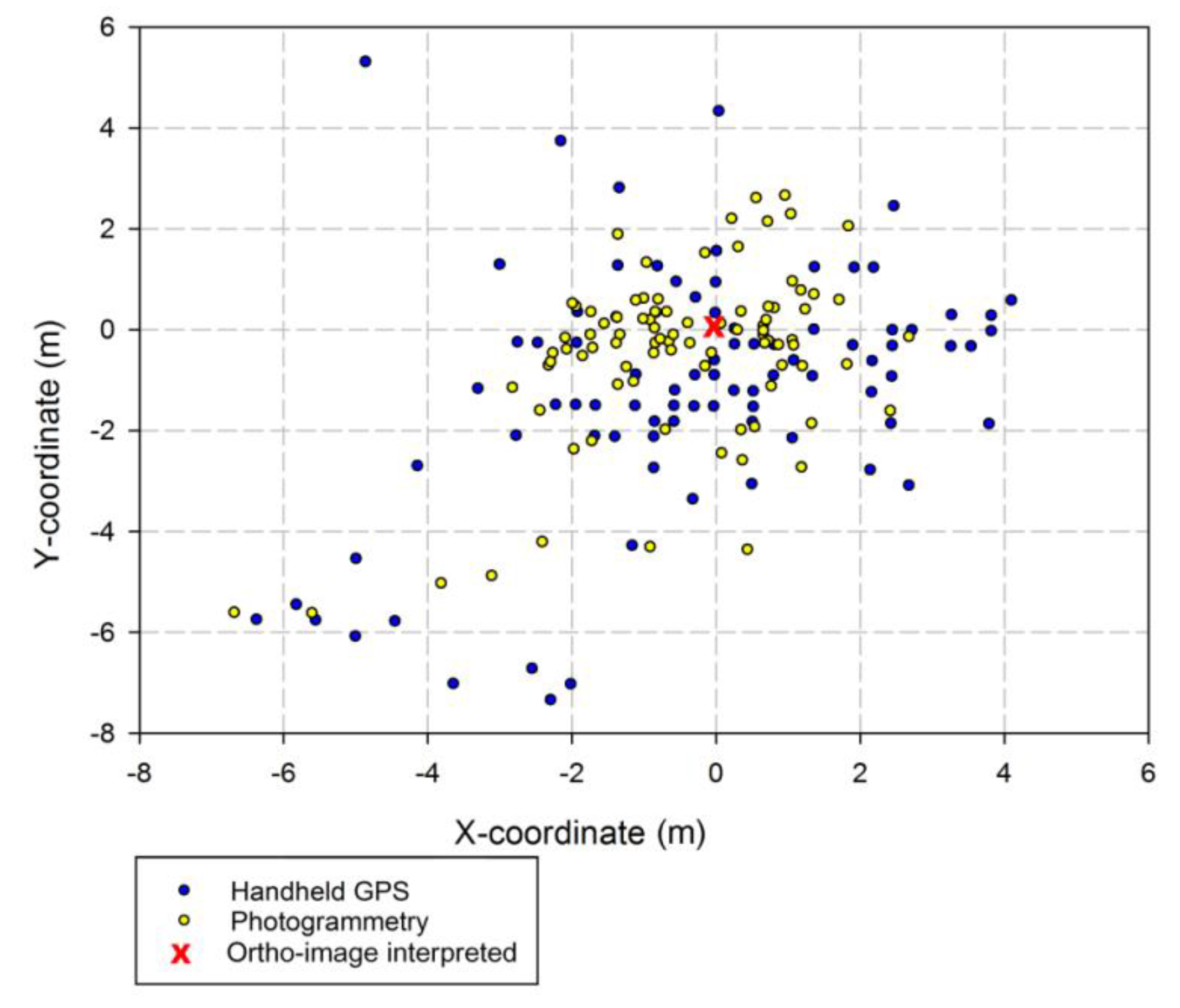
Both stationary and mobile measurements for DBH showed high conformity to their corresponding field measurements. The windbreak site showed an R2 value of 0.92 for stationary data and 0.95 for mobile data, while urban sites showed an R2 value of 0.98 for both stationary and mobile datasets (Figure 3).
Similarly, RMSE values showed relatively low error regardless of mobile or stationary treatment method and type of site. The windbreak site had very similar RMSE values of 1.24 cm (8.70%) and 1.06 cm (7.43%) for stationary and mobile datasets, respectively (Table 2). The urban sites had RMSE values of 2.81 cm (10.37%) and 2.18 cm (8.02%) for stationary and mobiles sites, respectively (Table 2).
Stationary-photographed urban stems showed a slightly greater bias at −1.80 cm (−6.64%), but the mobile urban bias was almost half that, at −0.98 cm (−3.60%) (Table 2). Bias for stems measured in windbreak sites was −0.54 cm (−3.78%) and −0.56 (−3.93%). Bias was consistently negative for all classifications and suggested the photogrammetric process, either in the point cloud generation or DBH mensuration routine, may lead to underestimation of DBH (i.e., −3.6% to −6.64%).

3.3. Stem Positions

In comparison to stem positions interpreted from the orthophoto images and field measurements, the photogrammetric and handheld GPS-derived stem positions were consistently negative along the X-axis for the windbreak site (Figure 4), while the positions were relatively more evenly-distributed around the orthophoto-interpreted positions for the urban sites (Figure 5). The average photogrammetric Y-measurement residuals were lower than the handheld-GPS for urban sites (i.e., by 0.53 m), but handheld-GPS had lower residuals for windbreak site (i.e., by 2.15 m) (Table 3). However, for the average X-coordinates residuals, the difference of the handheld-GPS was less than the photogrammetric model for the urban sites (i.e., by 0.18 m), the handheld-GPS showed lower average residuals than the photogrammetric model for the both the urban sites (i.e., by 0.18 m) and the windbreak sites (i.e., by 0.8 m) (Table 4).
The differences for both the handheld-GPS and photogrammetric coordinates showed relatively similar deviations from the orthophoto-interpreted stem positions for the urban site (Figure 5), but the handheld-GPS showed a more diffuse distribution for the X and Y stem coordinates for the windbreak site (Figure 4). At least under some conditions, which may indicate better precision from the photogrammetric model. Precision can be interpreted from the standard deviation of the differences. The handheld-GPS showed greater standard deviations (less precision) for both the windbreak and urban site X-coordinates (i.e., by 0.37 m and 0.77 m, respectively) and Y-coordinates (i.e., by 0.72 m and 0.68 m, respectively) (Table 3 and Table 4)—also suggesting that the photogrammetric method had higher precision.
Urban sites showed an overall greater range for Y-coordinates (i.e., residuals of −7.36–5.29 m for handheld GPS and −5.64–2.64 m for photogrammetry) than for the windbreak (i.e., −5.84 to −2.18 m for handheld GPS and −4.93 to −3.69 m for photogrammetry) (Table 3), which was similar for urban X-coordinates (i.e., −6.36–4.11 m for handheld GPS and −6.36–4.11 m for photogrammetry) relative to windbreak X-coordinates (i.e., −3.60 to −0.33 for handheld GPS and −3.63–1.64 m for photogrammetry) (Table 4).

4. Discussion

The mobile photogrammetric point cloud models in this study were suitably accurate for collecting DBH measurements, as seen with the strong correlation between the modeled and field-derived measurements (i.e., R2 < ~0.95) and relatively low error (RMSEs < 12.0%). These results compare favorably to field measurements, especially in light of evidence that high precision between individuals inventorying can be difficult to attain. For example, Kitahara et al. [58] showed the difference between median field DBH measurements between groups of inexperienced surveyors could significantly improve from 2.3% to 0.9% for conifers and 1.7% to 0.9% for broad-leaved trees with more training on basic sampling procedures. Luoma et al. [59] showed a standard deviation of 0.3 cm (1.5%) for DBH measurements taken independently by four experienced foresters in a boreal forest. In theory, physical tree measurements may necessitate high degrees of accuracy and precision, but past studies on SfM and terrestrial laser scanning data have generally concluded RMSEs of <10% are acceptable for most forest inventory purposes [39,45,46,48,53,60]. Given this precedent of acceptable error held by past studies on point cloud accuracy, measurements from this study compare well to previous applications of SfM photogrammetry for tree measurements (Table 1), as the RMSE value for DBH was <11% for both urban and windbreak sites (Table 2).
This study utilized many of the same techniques from past work on measuring trees with SfM point clouds like using high image overlap, high quantity of photos for the subjects being measured, and multiple angles for camera field of vision—but past terrestrial SfM studies have primarily operated within a local coordinate system with field-measured distances between specified reference points [45,46,48,60] or artificial targets [48] to scale the models. Alternatively, Surový et al. [49] used ground control points and a magnetic motion tracker points to georeference models via coordinates.
Unlike previous studies employing close-range photogrammetry for stem measurements, our mobile terrestrial photogrammetric set-up shared many features of mobile laser scanning since both do not rely on ground control points or local coordinate systems and scaling [61]. However, the mobile set-up in this study did not utilize an inertial measurement unit. These units are almost universally available in professional mobile laser scanning systems, and work in concert with the GPS to increase positional data accuracy. An inertial measurement unit is particularly important where GPS technology may become susceptible to signal related error (i.e., multipathing, occlusion, etc.), and urban areas can be challenging environments to record accurate data, due to the prevalence of tree canopy and large structures. Although the results in this study were not attained with an IMU, adding a unit to a similar set-up would likely enhance accuracy by compensating for poor satellite reception along highly-interrupted roadways.
Mobile laser scanning data is generally taken with the expressed intent of accuracy suitable for conventional property and infrastructure surveys (i.e., at the centimeter level of error). Street tree inventories do not typically require this level of positional accuracy to identify specific trees [10,31]. Tree positions along streets are often measured along the direction of the street based on the beginning of the block or the property boundary [31], hence, a similar technique was used in this study; however, this approach was modified to incorporate the use of ground objects and orthoimages. Unfortunately, the technique outlined in this paper using measurements of azimuth and distance from visible control objects to stems also has a major shortcoming, since orthoimages are often subject to georeferencing errors [62]. Such positional errors cause general localized directional shifts of the imagery relative to the physical coordinates of the depicted landscape and objects within the imagery. This may have been evidenced in the windbreak site, where stem positions taken from the handheld-GPS and the photogrammetric model showed consistent negative bias along the X-axis (Figure 4). The urban sites were distributed throughout the landscape of an entire city, and correspondingly, urban residuals were observed much less uniformly than the windbreak site (Figure 5), which may have been due to the use of multiple orthoimages having translational errors in a variety of different directions. Photogrammetric stem positions data showed higher-precision via associated standard deviations (Table 3 and Table 4).
Past close-range photogrammetry studies on individual tree measurements have typically incorporated 360° image coverage of trees to model all sides of the stems [45,46,48,49,53,60]. The vehicle-mounted photogrammetry system from this study exchanges overall coverage and favorable camera geometry for expediency. Similar to the limited perspective of a vehicle-mounted laser scanner, portions of the stems not facing the roadway were not modeled by mobile photogrammetry. However, mobile terrestrial photogrammetry differs from mobile laser scanning with regard to other advantages and limitations. The equipment used in this dataset is much less expensive than a vehicle outfitted with mobile laser scanning, as the creation of a georeferenced streetscape point cloud requires little more than a survey grade GPS, a timing GPS, two DSLR cameras, a laptop computer, a vehicle with a suitable mount, and a program license for SfM software [54]. Although the overall expense is less for mobile photogrammetry, there are still certain limitations associated with the SfM workflow. Relative to standard field measurements, photographic and geospatial data collection and model creation are still relatively work-intensive processes. The mobile photogrammetric system in this manuscript, and therefore the modeled area of the point cloud, are limited by camera field-of-vision.
Similar to mobile laser scanning data coverage, 360° reconstruction of stems was not possible; however, there was typically enough image coverage to measure the diameter from opposite sides of modeled stems (Figure 6). This roadside perspective is also typical of mobile laser scanning data, and measurements from these point clouds must be performed manually or from programmed circle-fitting functions [36]. Lack of perspective on irregularly shaped stems can lead to a potential source of error when measuring the diameter of a point cloud stem (Figure 6), and this can be particularly problematic for large stems, since their associated error is proportionally greater within a dataset.
Mobile laser scanning datasets can often produce models that account for the full height of trees, while stems modeled via mobile SfM photogrammetry in this experiment were limited by camera field-of-view. Some compensation may be available by adding more cameras to the mobile set-up. However, multiple georeferenced datasets can also be merged to potentially attain multiple biometrics that would otherwise be impossible to attain from stand-alone datasets (i.e., height from terrestrial and stem-related measurements from aerial). Omasa et al. [63] demonstrated this in an urban park with data taken from aerial and terrestrial LiDAR, but SfM point cloud dataset merges have also been performed from imagery captured independently from the ground and an unmanned aerial vehicle (UAV) [64]. Another possibility is to utilize imagery derived from unmanned aerial vehicles since the imagery can be taken at a gradient of heights from above and facing the sides of trees. Different combinations of imagery perspective were explored by Gatziolis et al. [65] to create SfM models for individual trees, and relatively uniform camera to tree distance was considered to be an important factor for creating SfM point clouds. Another advantage of mobile laser scanning datasets is their ability to account somewhat for woody portions of tree structure since some of the points can pass superficial leafy vegetation [66]—however, it is much more difficult for photogrammetric models to account for underlying woody structure during leaf-on conditions [66], or when they are occluded by nearby vegetation (Figure 7). Liang et al. [60], also noted that measurements from a SfM point cloud were generally inaccurate for stem measurements beyond 20 m from the camera, while unit specifications vary, mobile laser scanning datasets are generally considered accurate to a distance of 100 m before point densities significantly drop-off [67].
Processing imagery into point clouds suitable for measurements is relatively time-intensive. Processed SfM point clouds often have certain characteristics that can limit their overall usefulness. Residual error can occur from poor interpretation of depth, which typically presents itself as ‘artifact’ points from distant sources attached to other locations of the SfM model. When creating models along roadsides, the high overlap between photos (i.e., high volume of photos throughout the entire site) was important for maintaining continuity throughout the model. Trials leading to the utilized SfM methodology in this study showed poor reconstruction and continuity along the modeled right-of-way when not enough overlap between photos was present [54]. Post-processed dataset size is also a consideration, as SfM models tend to create much denser point clouds than mobile laser scanning. Terrestrial laser scanning data creates point clouds with much higher densities than aerial laser scanning data [68], but the amount of data associated with terrestrial-based SfM point clouds can be extremely cumbersome for computers to process and manipulate. Currently, mobile SfM photogrammetric datasets beyond a few hundred meters of roadway will typically overburden processing for consumer grade computers unless point densities are reduced [54]. The current solution to this problem is to process sections of roadway independently, and then to merge the point clouds after models have been created and evaluated to a user-defined level of acceptable accuracy.
Environmental conditions and camera settings can also highly impact the potential quality of the processed point cloud. Poor illumination and shadow in imagery can be difficult for computer programs to interpret [48,53]. Backgrounds with uniform composition, color, and texture can also be difficult for SfM software to interpret and model—particularly regarding depth (Figure 8). Vehicle speed is also a consideration, as the vehicle used in this manuscript had to travel at a relatively slow traffic speed of ~10 km/h. Occlusion and multipathing of satellite signals to GPS receivers can also result in relatively erroneous spatial data associated with image location. Future work in areas with canopy and tall buildings would greatly benefit from the inclusion of data from an inertial measurement unit.
Close-range remote sensing of roadways may see increasing utility with the proliferation of open-source and publicly available datasets. Currently, the most encompassing of existing street-level data is Google Street View, and existing survey and monitoring efforts assessed with Street View datasets likely illustrate a precedent for future work involving three-dimensional datasets from mobile laser scanning and mobile photogrammetry. There have been examples of using Google Street View to ascertain overall greenness [69] and to collect certain street tree parameters like species identification [70]. However, the use of Street View has been somewhat limited by its two-dimensional point of view, as Berland and Lange [70] also determined that it was not suitable for acquiring measurements. Google Street View imagery has already been demonstrated for cataloging and checking existing urban tree inventories [71] and as an additional means to identify trees by species when working with aerial and satellite data [72]. Inventories will likely become increasingly automated. Already, a machine learning approach utilizing publicly available aerial and street view imagery from Google Maps™ has been shown to detect street trees correctly and classify with >70% accuracy [73].

5. Conclusions

This research has demonstrated that close-range mobile terrestrial photogrammetry can be used for the purposes of mapping and basic tree measurements for inventory purposes. Modeled stem diameters correlated well with physical measurements. Tree position also compared favorably to observed coordinates from a handheld GPS unit. Mobile laser scanning has been an increasingly utilized technique for surveying roadways, and despite certain limitations to mobile photogrammetry (i.e., typically less model coverage, lack of superficial penetration, susceptibility to various sources of photogrammetric noise, typically denser datasets, etc.) the lower cost of cameras relative to LiDAR units and the relative ease of camera operation and image processing can provide an alternative to mobile laser scanning when certain advantages of mobile LiDAR are not necessary. The possibility that these terrestrial photogrammetric datasets can be merged with those from an aerial perspective may allow for more encompassing datasets for other tree measurements, advanced GIS analyses of roadside vegetation, and the inspection of other types roadside infrastructure. Comparison to mobile laser scanning, streamlining of data acquisition and processing, tests with other forest environments and inventory methods, and the automation of measurements from photogrammetric point clouds can provide further avenues to build on this research.

Author Contributions

Conceptualization, A.A.-E., A.K., B.W., J.R., G.H., S.L.; methodology, J.R., A.A.-E., A.P., B.W., S.L.; software, A.K., A.A.-E., B.W., J.R., and A.P.; validation, J.R., A.A.-E., and A.P.; formal analysis, J.R. and A.K.; investigation, J.R., A.K., and B.W.; resources, A.K., B.W., and A.A.-E.; data curation, J.R. and A.P.; writing—original draft preparation, J.R. and A.K.; writing—review and editing, A.A.-E., A.K., B.W., J.R., G.H., and S.L.; visualization, J.R., G.H., A.K.; supervision, A.K. and G.H.; project administration, A.K. and J.R.; funding acquisition, A.K.

Funding

This research received no external funding.

Acknowledgments

The authors would like to thank Drew McLean and H. Andrew Lassiter for their assistance and insight on this project. Financial support was partially provided by the University of Florida-IFAS Center for Landscape Conservation and Ecology and the Garden Club of America Zone VI Fellowship in Urban Forestry.

Conflicts of Interest

The authors declare no conflict of interest.

References

  1. Roy, S.; Byrne, J.; Pickering, C. A systematic quantitative review of urban tree benefits, costs, and assessment methods across cities in different climatic zones. Urban For. Urban Green. 2012, 11, 351–363. [Google Scholar] [CrossRef] [Green Version]
  2. Seamans, G.S. Mainstreaming the environmental benefits of street trees. Urban For. Urban Green. 2013, 12, 2–11. [Google Scholar] [CrossRef]
  3. Nowak, D.; Crane, D.; Stevens, J.; Hoehn, R.; Walton, T.; Bond, J. A ground-based method of assessing urban forest structure and ecosystem services. Arboric. Urban For. 2008, 34, 347–358. [Google Scholar]
  4. Hauer, R.; Vogt, J.; Fischer, B. The cost of not maintaining the urban forest. Arborist News. 2015, 24, 12–19. [Google Scholar]
  5. Vogt, J.; Hauer, R.; Fischer, B. The Costs of Maintaining and Not Maintaining the Urban Forest: A Review of the Urban Forestry and Arboriculture Literature. Arboric. Urban For. 2015, 41, 293–323. [Google Scholar]
  6. Keller, J.; Konijnendijk, C. Short communication: A comparative analysis of municipal urban tree inventories of selected major cities in North America and Europe. Arboric. Urban For. 2012, 38, 24–30. [Google Scholar]
  7. Roman, L.; McPherson, E.; Scharenbroch, B.; Bartens, J. Identifying common practices and challenges for local urban tree monitoring programs across the United States. Arboric. Urban For. 2013, 39, 292–299. [Google Scholar]
  8. Bond, J. Tree Inventories; International Society of Arboriculture: Atlanta, GA, USA, 2013. [Google Scholar]
  9. Östberg, J.; Delshammar, T.; Wiström, B.; Nielsen, A. Grading of parameters for urban tree inventories by city officials, arborists, and academics using the Delphi method. Environ. Manag. 2013, 51, 694–708. [Google Scholar] [CrossRef]
  10. Maco, S.; McPherson, E. A practical approach to assessing structure, function, and value of street tree populations in small communities. J. Arboric. 2003, 29, 84–97. [Google Scholar]
  11. Koeser, A.K.; Hauer, R.J.; Miesbauer, J.W.; Peterson, W. Municipal tree risk assessment in the United States: Findings from a comprehensive survey of urban forest management. Arboric. J. 2016, 38, 1–12. [Google Scholar] [CrossRef]
  12. Ward, K.T.; Johnson, G.R. Geospatial methods provide timely and comprehensive urban forest information. Urban For. Urban Green. 2007, 6, 15–22. [Google Scholar] [CrossRef]
  13. Dwyer, M.; Miller, R. Using GIS to assess urban tree canopy benefits and surrounding greenspace distributions. J. Arboric. 1999, 25, 102–107. [Google Scholar]
  14. Walton, J.; Nowak, J.; Greenfield, J. Assessing urban forest canopy cover using airborne or satellite imagery. Arboric. Urban For. 2008, 34, 334–340. [Google Scholar]
  15. Sander, H.; Polasky, S.; Haight, R.G. The value of urban tree cover: A hedonic property price model in Ramsey and Dakota Counties, Minnesota, USA. Ecol. Econ. 2010, 69, 1646–1656. [Google Scholar] [CrossRef]
  16. Wu, C.; Xiao, Q.; McPherson, E.G. A method for locating potential tree-planting sites in urban areas: A case study of Los Angeles, USA. Urban For. Urban Green. 2008, 7, 65–76. [Google Scholar] [CrossRef]
  17. Locke, D.; Grove, J.; Lu, J.; Troy, A.; O’Neil-Dunne, J.; Beck, B. Prioritizing preferable locations for increasing urban tree canopy in New York City. Cities Environ. CATE 2011, 3, 4. [Google Scholar]
  18. Abd-Elrahman, A.H.; Thornhill, M.E.; Andreu, M.G.; Escobedo, F. A community-based urban forest inventory using online mapping services and consumer-grade digital images. Int. J. Appl. Earth Obs. Geoinf. 2010, 12, 249–260. [Google Scholar] [CrossRef]
  19. Pu, R.; Landry, S. A comparative analysis of high spatial resolution IKONOS and WorldView-2 imagery for mapping urban tree species. Remote Sens. Environ. 2012, 124, 516–533. [Google Scholar] [CrossRef]
  20. Clark, M.L.; Roberts, D.A.; Clark, D.B. Hyperspectral discrimination of tropical rain forest tree species at leaf to crown scales. Remote Sens. Environ. 2005, 96, 375–398. [Google Scholar] [CrossRef]
  21. Bunting, P.; Lucas, R. The delineation of tree crowns in Australian mixed species forests using hyperspectral Compact Airborne Spectrographic Imager (CASI) data. Remote Sens. Environ. 2006, 101, 230–248. [Google Scholar] [CrossRef]
  22. Koch, B.; Heyder, U.; Weinacker, H. Detection of individual tree crowns in airborne LiDAR data. Photogramm. Eng. Remote Sens. 2006, 72, 357–363. [Google Scholar] [CrossRef]
  23. Lee, A.C.; Lucas, R.M. A LiDAR-derived canopy density model for tree stem and crown mapping in Australian forests. Remote Sens. Environ. 2007, 111, 493–518. [Google Scholar] [CrossRef]
  24. Tanhuanpää, T.; Vastaranta, M.; Kankare, V.; Holopainen, M.; Hyyppä, J.; Hyyppä, H.; Alho, P.; Raisio, J. Mapping of urban roadside trees—A case study in the tree register update process in Helsinki City. Urban For. Urban Green. 2014, 13, 562–570. [Google Scholar] [CrossRef]
  25. Zhang, C.; Qiu, F. Mapping individual tree species in an urban forest using airborne LiDAR data and hyperspectral imagery. Photogramm. Eng. Remote Sens. 2012, 78, 1079–1087. [Google Scholar] [CrossRef]
  26. Alonzo, M.; Bookhagen, B.; Roberts, D. Urban tree species mapping using hyperspectral and LiDAR data fusion. Remote Sens. Environ. 2014, 148, 70–83. [Google Scholar] [CrossRef]
  27. Lee, J.H.; Ko, Y.; McPherson, E.G. The feasibility of remotely sensed data to estimate urban tree dimensions and biomass. Urban For. Urban Green. 2016, 16, 208–220. [Google Scholar] [CrossRef] [Green Version]
  28. Alonzo, M.; McFadden, J.; Nowak, D.; Roberts, D. Mapping urban forest structure and function using hyperspectral imagery and LiDAR data. Urban For. Urban Green. 2016, 17, 135–147. [Google Scholar] [CrossRef]
  29. Nielsen, A.; Östberg, J.; Delshammar, T. Review of Urban Tree Inventory Methods Used to Collect Data at Single-Tree Level. Arboric. Urban For. 2014, 40, 96–111. [Google Scholar]
  30. Wu, J.; Yao, W.; Polewski, P. Mapping Individual Tree Species and Vitality along Urban Road Corridors with LiDAR and Imaging Sensors: Point Density versus View Perspective. Remote Sens. 2018, 10, 1403. [Google Scholar] [CrossRef]
  31. Singh, K.; Gagné, S.; Meentemeyer, R. Comprehensive Remote Sensing, Chapter: 9.22. In Urban Forests and Human Well-Being; Liang, S.L., Ed.; Elsevier: Amsterdam, The Netherlands, 2018; pp. 287–305. [Google Scholar] [CrossRef]
  32. Fröhlich, C.; Mettenleiter, M. Terrestrial laser scanning—New perspectives in 3D surveying. Int. Arch. Photogramm. Remote Sens. Spat. Inf. Sci. 2004, 36, W2. [Google Scholar]
  33. Watt, P.J.; Donoghue, D.N.M. Measuring forest structure with terrestrial laser scanning. Int. J. Remote Sens. 2005, 26, 1437–1446. [Google Scholar] [CrossRef]
  34. Abellan, A.; Vilaplana, J.; Martinez, J. Application of a long-range Terrestrial Laser Scanner to a detailed rockfall study at Vall de Núria (Eastern Pyrenees, Spain). Eng. Geol. 2006, 88, 136–148. [Google Scholar] [CrossRef]
  35. Lerma, J.L.; Navarro, S.; Cabrelles, M.; Villaverde, V. Terrestrial laser scanning and close range photogrammetry for 3D archaeological documentation: The Upper Palaeolithic Cave of Parpalló as a case study. J. Archaeol. Sci. 2010, 37, 499–507. [Google Scholar] [CrossRef]
  36. Van Leeuwen, M.; Nieuwenhuis, M. Retrieval of forest structural parameters using LiDAR remote sensing. Eur. J. For. Res. 2010, 129, 749–770. [Google Scholar] [CrossRef]
  37. Moskal, L.M.; Zheng, G. Retrieving Forest Inventory Variables with Terrestrial Laser Scanning (TLS) in Urban Heterogeneous Forest. Remote Sens. 2011, 4, 1–20. [Google Scholar] [CrossRef] [Green Version]
  38. Yao, W.; Krzystek, P.; Heurich, M. Tree species classification and estimation of stem volume and DBH based on single tree extraction by exploiting airborne full-waveform LiDAR data. Remote Sens. Environ. 2012, 123, 368–380. [Google Scholar] [CrossRef]
  39. Henning, J.; Radtke, P. Detailed stem measurements of standing trees from ground-based scanning LiDAR. For. Sci. 2006, 52, 67–80. [Google Scholar] [CrossRef]
  40. Williams, K.; Olsen, M.; Roe, G.; Glennie, C. Synthesis of transportation applications of mobile LiDAR. Remote Sens. 2013, 5, 4652–4692. [Google Scholar] [CrossRef]
  41. Holopainen, M.; Kankare, V.; Vastaranta, M.; Liang, X.; Lin, Y.; Vaaja, M.; Yu, X.; Hyyppä, J.; Hyyppä, H.; Kaartinen, H.; et al. Tree mapping using airborne, terrestrial and mobile laser scanning—A case study in a heterogeneous urban forest. Urban For. Urban Green. 2013, 12, 546–553. [Google Scholar] [CrossRef]
  42. Dandois, J.P.; Ellis, E.C. High spatial resolution three-dimensional mapping of vegetation spectral dynamics using computer vision. Remote Sens. Environ. 2013, 136, 259–276. [Google Scholar] [CrossRef] [Green Version]
  43. Lisein, J.; Pierrot-Deseilligny, M.; Bonnet, S.; Lejeune, P. A Photogrammetric Workflow for the Creation of a Forest Canopy Height Model from Small Unmanned Aerial System Imagery. Forests 2013, 4, 922–944. [Google Scholar] [CrossRef] [Green Version]
  44. Zarco-Tejada, P.J.; Diaz-Varela, R.; Angileri, V.; Loudjani, P. Tree height quantification using very high resolution imagery acquired from an unmanned aerial vehicle (UAV) and automatic 3D photo-reconstruction methods. Eur. J. Agron. 2014, 55, 89–99. [Google Scholar] [CrossRef]
  45. Morgenroth, J.; Gomez, C. Assessment of tree structure using a 3D image analysis technique—A proof of concept. Urban For. Urban Green. 2014, 13, 198–203. [Google Scholar] [CrossRef]
  46. Miller, J.; Morgenroth, J.; Gomez, C. 3D modelling of individual trees using a handheld camera: Accuracy of height, diameter and volume estimates. Urban For. Urban Green. 2015, 14, 932–940. [Google Scholar] [CrossRef]
  47. Bauwens, S.; Foyelle, A.; Gourlet-Fleury, S.; Ndjele, L.; Mengal, C.; Lejeune, P. Terrestrial photogrammetry: A non-destructive method for modelling irregularly shaped tropical tree trunks. Methods Ecol. Evol. 2017, 8, 460–471. [Google Scholar] [CrossRef]
  48. Liang, X.; Jaakkola, A.; Wang, Y.; Hyyppa, J.; Honkavaara, E.; Liu, J.; Kaartinen, H. The Use of a Hand-Held Camera for Individual Tree 3D Mapping in Forest Sample Plots. Remote Sens. 2014, 6, 6587–6603. [Google Scholar] [CrossRef] [Green Version]
  49. Surový, P.; Yoshimoto, A.; Panagiotidis, D. Accuracy of Reconstruction of the Tree Stem Surface Using Terrestrial Close-Range Photogrammetry. Remote Sens. 2016, 8, 123. [Google Scholar] [CrossRef]
  50. Mikita, T.; Janata, P.; Surový, P. Forest Stand Inventory Based on Combined Aerial and Terrestrial Close-Range Photogrammetry. Forests 2016, 7, 165. [Google Scholar] [CrossRef]
  51. Mokroš, M.; Liang, X.; Surový, P.; Valent, P.; Čerňava, J.; Chudý, F.; Tunák, D.; Saloň, Š.; Merganič, J. Evaluation of close-range photogrammetry image collection methods for estimating tree diameters. ISPRS Int. J. Geo Inf. 2018, 7, 93. [Google Scholar] [CrossRef]
  52. Mokroš, M.; Výbošťok, J.; Tomaštík, J.; Grznárová, A.; Valent, P.; Slavik, M.; Merganič, J. High precision individual tree diameter and precision estimation from close-range photogrammetry. Forests 2018, 9, 696. [Google Scholar] [CrossRef]
  53. Koeser, A.K.; Roberts, J.W.; Miesbauer, J.W.; Lopes, A.B.; Kling, G.J.; Lo, M.; Morgenroth, J. Testing the accuracy of imaging software for measuring tree root volumes. Urban For. Urban Green. 2016, 18, 95–99. [Google Scholar] [CrossRef]
  54. Roberts, J.W.; Koeser, A.K.; Abd-Elrahman, A.H.; Hansen, G.; Landry, S.M.; Wilkinson, B.E. Terrestrial photogrammetric stem mensuration for street trees. Urban For. Urban Green. 2018, 35, 66–71. [Google Scholar] [CrossRef]
  55. Abd-Elrahman, A.; Pande-Chhetri, R.; Vallad, G. Design and Development of a Multi-Purpose Low-Cost Hyperspectral Imaging System. Remote Sens. 2011, 3, 570–586. [Google Scholar] [CrossRef] [Green Version]
  56. Abd-Elrahman, A.; Sassi, N.; Wilkinson, B.; DeWitt, B. Georeferencing of mobile ground-based hyperspectral digital single-lens reflex imagery. J. Appl. Remote Sens. 2016, 10, 14002. [Google Scholar] [CrossRef] [Green Version]
  57. Microsoft Corporation. Microsoft Excel 2010 (V14.0); Microsoft Corporation: Redmond, WA, USA, 2010. [Google Scholar]
  58. Kitahara, F.; Mizoue, N.; Yoshida, S. Effects of training for inexperienced surveyors on data quality of tree diameter and height measurements. Silva Fenn. 2010, 44, 657–667. [Google Scholar] [CrossRef]
  59. Luoma, V.; Saarinen, N.; Wulder, M.A.; White, J.C.; Vastaranta, M.; Holopainen, M.; Hyyppä, J. Assessing Precision in Conventional Field Measurements of Individual Tree Attributes. Forests 2017, 8, 38. [Google Scholar] [CrossRef]
  60. Liang, X.; Wang, Y.; Jaakkola, A.; Kukko, A.; Kaartinen, H.; Hyyppä, J.; Honkavaara, E.; Liu, J. Forest Data Collection Using Terrestrial Image-Based Point Clouds from a Handheld Camera Compared to Terrestrial and Personal Laser Scanning. IEEE Trans. Geosci. Remote Sens. 2015, 53, 1–16. [Google Scholar] [CrossRef]
  61. Daneshmand, M.; Helmi, A.; Avots, E.; Noroozi, F.; Alisinanoglu, F.; Sait Arslan, H.; Gorbova, J.; Haamer, R.; Ozcinar, C.; Anbarjafari, G. 3D scanning: A comprehensive survey. Scand. J. For. Res. 2018, 30, 73–86. [Google Scholar]
  62. Bertin, S.; Friedrich, H.; Delmas, H.; Chan, E.; Gimel’farb, G. Digital stereo photogrammetry for grain-scale monitoring of fluvial surfaces: Error evaluation and workflow optimization. ISPRS J. Photogramm. Remote Sens. 2015, 101, 193–208. [Google Scholar] [CrossRef]
  63. Omasa, K.; Hosoi, F.; Uenishi, T.; Shimizu, Y.; Akiyama, Y. Three-dimensional modeling of an urban park and trees by combined airborne and portable on-ground scanning LIDAR remote sensing. Environ. Modeling Assess. 2008, 13, 473–481. [Google Scholar] [CrossRef]
  64. Lassiter, H.; Wilkinson, B. Comparison of terrestrial 3D mapping methods for urban forest parameters. In Proceedings of the International LiDAR Mapping Forum, Denver, CO, USA, 22–24 February 2016. [Google Scholar]
  65. Gatziolis, D.; Lienard, J.F.; Vogs, A.; Strigul, N.S. 3D Tree Dimensionality Assessment Using Photogrammetry and Small Unmanned Aerial Vehicles. PLoS ONE 2015, 10, e0137765. [Google Scholar] [CrossRef]
  66. White, J.C.; Coops, N.C.; Wulder, M.A.; Vastaranta, M.; Hilker, T.; Tompalski, P. Remote Sensing Technologies for Enhancing Forest Inventories: A Review. Can. J. Remote Sens. 2016, 42, 619–641. [Google Scholar] [CrossRef] [Green Version]
  67. Puente, I.; González-Jorge, H.; Martínez-Sánchez, J.; Arias, P. Review of mobile mapping and surveying technologies. Measurement 2013, 46, 2127–2145. [Google Scholar] [CrossRef]
  68. Fritz, A.; Kattenborn, T.; Koch, B. Uav-Based Photogrammetric Point Clouds—Tree Stem Mapping in Open Stands in Comparison to Terrestrial Laser Scanner Point Clouds. ISPRS Int. Arch. Photogramm. Remote Sens. Spat. Inf. Sci. 2013, 40, 141–146. [Google Scholar] [CrossRef]
  69. Li, X.J.; Zhang, C.; Li, W.; Ricard, R.; Meng, Q.; Zhang, W. Assessing street-level urban greenery using Google Street View and a modified green view index. Urban For. Urban Green. 2015, 14, 675–685. [Google Scholar] [CrossRef]
  70. Berland, A.; Lange, D.A. Google Street View shows promise for virtual street tree surveys. Urban For. Urban Green. 2017, 21, 11–15. [Google Scholar] [CrossRef]
  71. Wegner, J.; Branson, S.; Hall, D.; Schindler, K.; Perona, P. Cataloging public objects using aerial and street level images—Urban trees. In Proceedings of the the IEEE Conference on Computer Vision and Pattern Recognition, Las Vegas, NV, USA, 27–30 June 2016; pp. 6014–6023. [Google Scholar]
  72. Alvarez, I.; Gallo, B.; Garçon, E.; Oshiro, O. Street tree inventory of Campinas, Brazil: An instrument for urban forestry management and planning. Arboric. Urban For. 2015, 41, 233–244. [Google Scholar]
  73. Branson, S.; Wegner, J.D.; Hall, D.; Lang, N.; Schindler, K.; Perona, P. From Google Maps to a fine-grained catalog of street trees. ISPRS J. Photogramm. Remote Sens. 2018, 135, 13–30. [Google Scholar] [CrossRef] [Green Version]
Figure 1. Schematic of the experimental stereoscopic mobile camera set-up. Representation of image capture with a mobile vehicle (left) and stationary image capture with a surveying pole (right).
Forests 10 00701 g001
Figure 2. Mounted vehicle set-up used for mobile photogrammetry in this study.
Forests 10 00701 g002
Figure 3. Comparison between stationary and mobile data based on site classification.
Forests 10 00701 g003
Figure 4. Comparison between handheld GPS and mobile photogrammetric tree X and Y coordinates relative to the orthoimage-interpreted stem positions for the windbreak site.
Forests 10 00701 g004
Figure 5. Comparison between handheld GPS and mobile photogrammetric X and Y coordinates relative to orthoimage-interpreted stem positions for urban sites.
Forests 10 00701 g005
Figure 6. Point cloud stem slices used for measuring a highly-circular stem (left) and irregular-shaped stems (center and right).
Forests 10 00701 g006
Figure 7. An individual photo of a stem occluded by vegetation (left), the point cloud model of the stem (center), and the resulting diameter at breast height slice from this tree (right).
Forests 10 00701 g007
Figure 8. A stem modeled in PhotoScan with a highly uniform background. (A) A point cloud of a stem from the perspective of the roadway; (B) an image of the stem used to create the point cloud; (C) the stem from the perspective of above demonstrating error points around the stem from poor depth discrimination from the nearby background; (D) the stem from the perspective of the roadway demonstrating error points around the stem from poor depth discrimination from the nearby background.
Forests 10 00701 g008
Table 1. Comparison of tree features modeled with close-range photogrammetry.
StudyFeatureRMSE (%)RMSE in UnitsAccuracy
Bauwens et al. (2017)stem diameter4.5–4.65.8–5.9 cm-
Koeser et al. (2016)root system volume12.340.37 cm3-
Liang et al. (2014)DBH6.62.39 cm-
tree detection rate--88%
Mikita et al. (2016)tree positional accuracy--0.071—0.951 m
DBH-0.911–1.797 cm-
stem volume-0.082–0.180 m3-
Miller et al. (2015)DBH9.60.99 mm-
height3.745.15 cm-
crown spread14.764.1 cm-
crown depth11.932.53 cm-
stem volume12.33115.45 cm3-
branch volume47.53138.59 cm3-
total volume18.53266.79 cm3-
Mokroš et al. (2018)tree detection rate--80.60%
Mokroš et al. (2018)stem diameter0.9–1.85--
stem perimeter0.21–0.99--
Morgenroth and Gomez (2014)DBH3.73 cm-
height2.599 cm-
Roberts et al. (2018)DBH7.04–12.350.97–3.10 cm-
Surový et al. (2016)DBHNA0.59 cm-
Table 2. A comparison between field-measured and modeled diameter at breast height for urban (n = 88) and windbreak (n = 52) trees.
SiteDataMeanfield-measured (cm)Meanmodeled (cm)RMSE (cm)RMSE (%)Bias (cm)Bias (%)
Urban (n = 88)Stationary27.1325.322.8110.37−1.80−6.64
Mobile27.1326.152.188.02−0.98−3.60
Windbreak (n = 52)Stationary14.2113.681.248.70−0.54−3.78
Mobile14.2113.651.067.43−0.56−3.93
Table 3. A comparison of Y-coordinate differences for tree positions between satellite interpreted coordinates from handheld GPS (HH-GPS) and photogrammetry (Photo.).
SiteData Mean Residual (m)Standard Deviation (m)Min. (m)Max. (m)
Urban (n = 88)HH-GPS Y−1.17 (0.25) *2.38−7.365.29
Photo. Y−0.49 (0.18) *1.70−5.642.64
Windbreak (n = 52)HH-GPS Y−2.23 (0.20) *1.42−5.842.18
Photo. Y−4.38 (0.05) *0.35−4.93−3.69
* Standard error.
Table 4. A comparison of X-coordinate differences for tree positions between satellite interpreted coordinates from field-based GPS and photogrammetry.
SiteData Mean Residual (m)Standard Deviation (m)Min. (m)Max. (m)
UrbanHH-GPS X−0.30 (0.25) *2.36−6.364.11
Photo. X−0.48 (0.17) *1.59−6.672.69
WindbreakHH-GPS X−2.15 (0.09) *0.70−3.6−0.33
Photo. X−2.95 (0.05) *0.33−3.63−1.64
* Standard error.

