Large Area Forest Yield Estimation with Pushbroom Digital Aerial Photogrammetry

Abstract

Low-cost methods to measure forest structure are needed to consistently and repeatedly inventory forest conditions over large areas. In this study we investigate low-cost pushbroom Digital Aerial Photography (DAP) to aid in the estimation of forest volume over large areas in Washington State (USA). We also examine the effects of plot location precision (low versus high) and Digital Terrain Model (DTM) resolution (1 m versus 10 m) on estimation performance. Estimation with DAP and post-stratification with high-precision plot locations and a 1 m DTM was 4 times as efficient (precision per number of plots) as estimation without remote sensing and 3 times as efficient when using low-precision plot locations and a 10 m DTM. These findings can contribute significantly to efforts to consistently estimate and map forest yield across entire states (or equivalent) or even nations. The broad-scale, high-resolution, and high-precision information provided by pushbroom DAP facilitates used by a wide variety of user types such a towns and cities, small private timber owners, fire prevention groups, Non-Governmental Organizations (NGOs), counties, and state and federal organizations.

1. Introduction

The Forest Inventory and Analysis program (FIA; see also Appendix A, Glossary of terminology and statistical notation) within the US Forest Service (USFS) maintains and manages the national grid of forest inventory plots for the United States [1]. It comprises a grid of fixed area plots designed to cover the USA, with an approximate sampling intensity of one plot per 2430 ha [2]. This rich data resource is designed to support inferences from areas as broad as entire states down to individual counties. There are a variety of applications, however, that would benefit from consistent and precise forest measurements and monitoring across the USA at a finer than county resolution. Applications include (e.g.) mapping and small area estimation of fuels, forest yield, cover, and change. Researchers have mapped forest attributes over broad areas at moderate to fine resolutions with satellite-based imagery, such as MODIS and LANDSAT [3,4]. These products are improvements in the sense of providing higher-resolution spatial maps, but they have limited ability to quantify variation in vertical forest structure relative to what is feasible with remote sensing technologies such as lidar and photogrammetry. Lidar capabilities have been widely demonstrated to model forest height [5], volume [6], biomass [7], carbon [8], canopy fuels [9], and other height and cover related forest attributes [10].

While lidar has proven effective for modeling a variety of vertical structure related forest attributes, a well-known limitation of lidar is its high cost, especially at the scale of entire states. Recent lidar prices in the USA typically range from approximately $0.40/ha to $7/ha. Even at the low end, it would cost approximately 125 million USD to cover all USA forests a single time. While there is currently an effort underway by the USGS [11] to acquire nationwide lidar coverage, it is a long term project, and the return interval may exceed what is useful for monitoring vegetation. Digital Areal Photogrammetry (DAP) is an alternative remote sensing technology which also has the capacity to support large-area forest structure measurements. This technology is commonly referred to by a number of names including Structure from Motion (SfM) and, colloquially, phodar, an inaccurate combination of the term “photo” in photogrammery and Detection and Ranging “DAR” from lidar. The imagery used to support DAP can range in price from less than $0.01/ha as an in an archival project to over $2 USD/ha depending on acquisition specifications. For example, new stereo imagery which is used for the National Agriculture Imagery Program (NAIP) is available every 2–3 years over the entire conterminous USA, and requesting digital surfaces models for the acquisitions costs less than $0.01/ha.

DAP-based measurements of forest structure have been shown to be slightly worse than lidar in terms of performance for measurements such as height, basal area, and volume [12,13,14]. However, unlike lidar, a requirement for using DAP effectively is to have an alternative source for a Digital Terrain Model (DTM) because DAP typically measures the first surface, and therefore does not measure the ground surface beneath vegetation. In contrast, lidar can provide both measurements of the vertical forest structure and a detailed representation of the ground surface. Lidar data in the public domain can serve as a reliable source of DTMs for DAP, but much of the USA is not covered with lidar. An alternative source of DTMs for the USA is the US Geological Survey (USGS) National Elevation Dataset (NED) which is derived from diverse sources and “… is a seamless dataset with the best available raster elevation data of the conterminous United States, Alaska, Hawaii, and territorial islands” [15]. The NED rasters for the USA are approximately 10 m horizontal resolution and 1.5 m–2.4 m vertical RMSE [16]. NED elevations are inferior to most modern lidar acquisitions with respect to resolution and vertical accuracy, but they are often the best free source of DTMs for expansive areas in the USA. One question of interest then, is how well the USGS NED DTM can be used with DAP to support forest inventory applications.

For this study, DAP was derived from airborne pushbroom sensor imagery. The motivation to collect data with pushbroom sensors is their wide swath width and multiple look angles, which support stereo (from two look angles) from a single over-flight. A noted limitation with pushbroom imagery relative to frame imagery is increased difficulty to extract a detailed, artifact-free canopy surface model. Artifacts include smoothing or omission of surface features such as lone trees, canopy edges, and canopy gaps. The challenges encountered with pushbroom imagery are discussed in greater detail in the methods section.

The objective of this investigation is to evaluate forest yield estimation with pushbroom DAP and FIA field measurements. The performances of the DAP-based methods were assessed by determining whether estimation with auxiliary height information increased the efficiency (estimated variation relative to sample size) of estimation. Multiple components of the estimation strategy are examined, including the estimator used (regression versus post-stratification), plot positioning accuracy (low versus high), and the source of DTM (lidar versus NED).

2. Methods

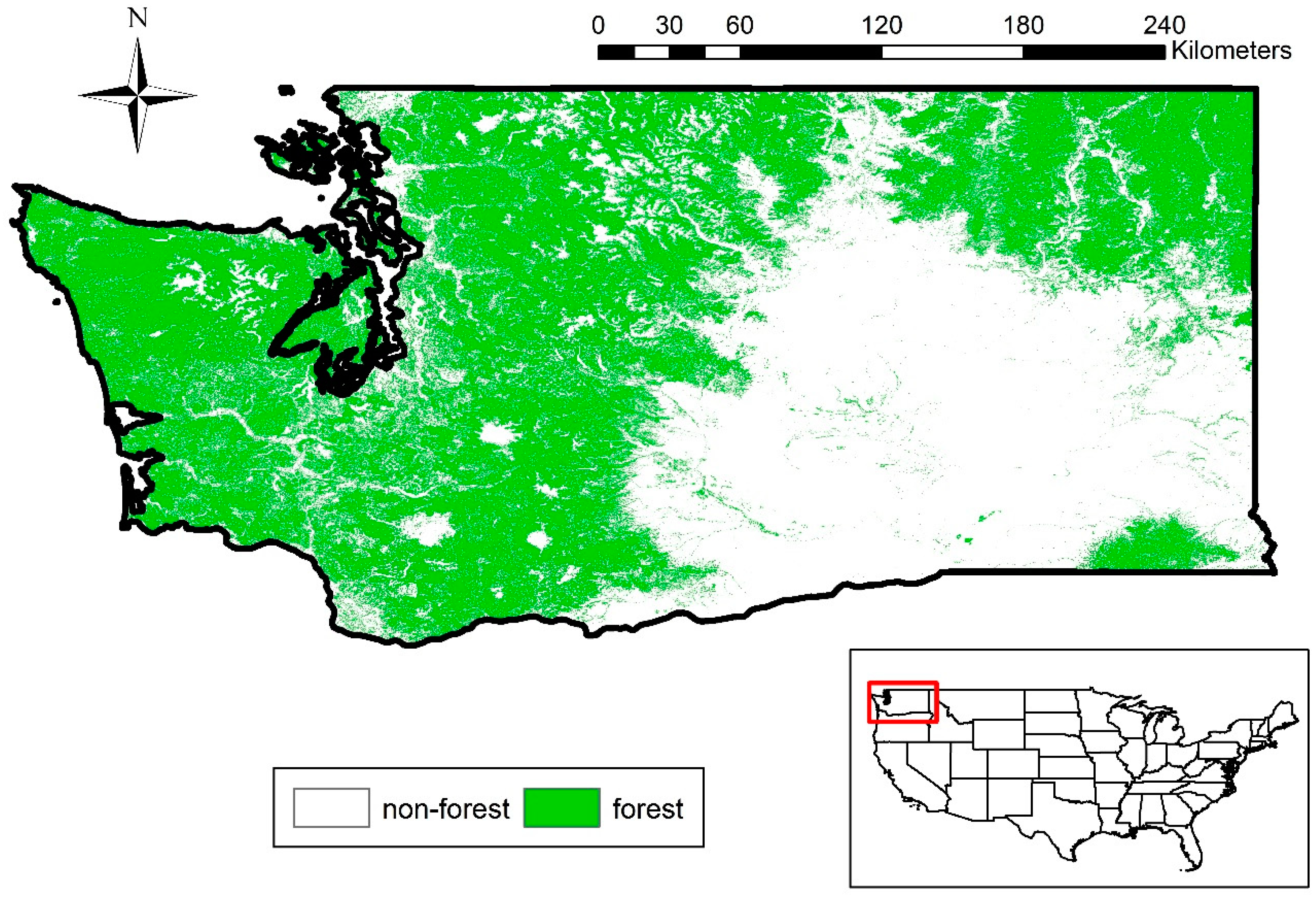
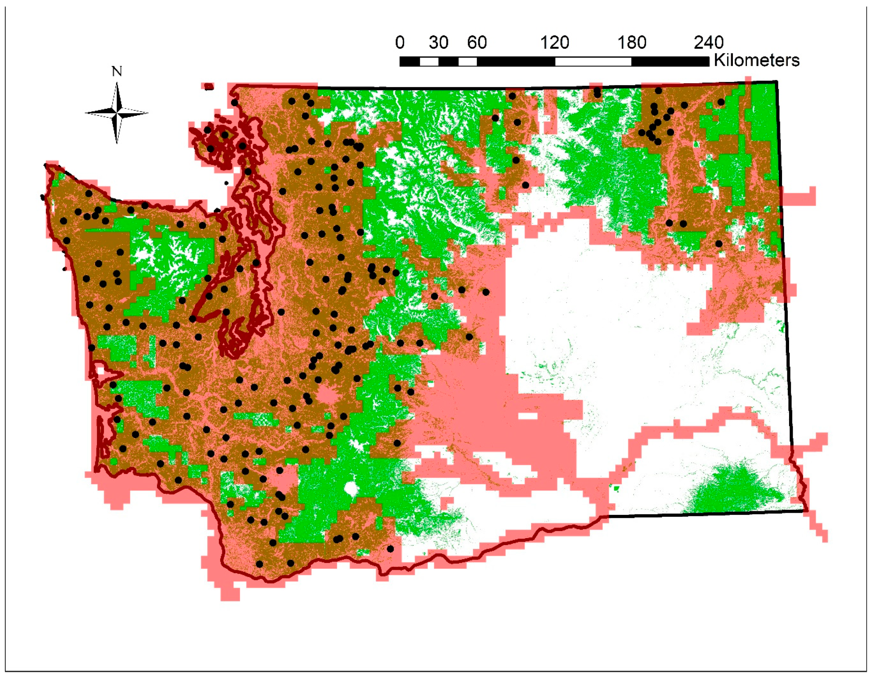
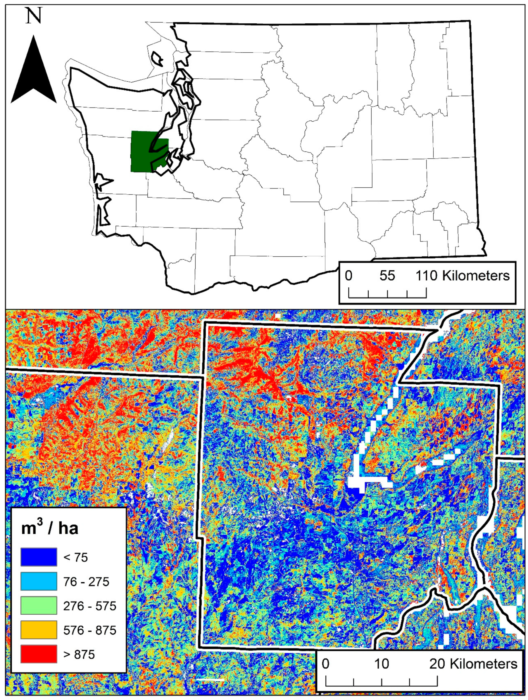
Study Site

This study was conducted for forested areas in the state of Washington (Figure 1), the Northwestern-most state of the conterminous USA. Washington State is a complex mixture of forest and non-forest conditions that spans extreme moisture and elevation gradients, including temperate rainforest, shrub-steppe, desert, alpine forest, five or more mountain ranges, and numerous volcanic peaks, including Mount Rainier, which rises from near sea level to 4352 m. Washington forests are dominated by conifer species such as Douglas fir (Pseudotsuga menziesii (Mirb.) Franco), Western hemlock (Tsuga heterophylla (Raf.) Sarg.), Western redcedar (Thuja plicata Donn), Sitka spruce (Picea sitchensis (Bong.) Carrière), ponderosa pine (Pinus ponderosa Lawson & C. Lawson), lodgepole pine (Pinus contorta Douglas ex Loudon), Western white pine (Pinus monticola Douglas ex D. Don), Alaskan yellow cedar (Callitropsis nootkatensis (D. Don) Oerst. ex D.P. Little), and various species of true firs (Abies), primarily at higher elevation. Common broad-leaved trees include Western red alder (Alnus rubra Bong.), bigleaf maple (Acer macrophyllum Pursh), black cottonwood (Populus balsamifera L. ssp. trichocarpa (Torr. & A. Gray ex Hook.) Brayshaw), Pacific madrona (Arbutus menziesii Pursh), Oregon white oak (Quercus garryana Douglas ex Hook.), paper birch (Betula papyrifera Marshall), and quaking aspen (Populus tremuloides Michx.).

3. Data

3.1. Field Measurements

Field measurements for this study were collected on Forest Inventory and Analysis (FIA) forest inventory plots measured by the USFS. Measurements in Washington state are taken annually over a 10 year period, but paneled such that inference can be made from FIA measurements taken in any given year (where a panel consists of a regularly spaced subset of the full grid; see Reference ([2] p. 20) for an expanded explanation of panels). The observations used for this study were measured during the 2015 field season.

3.2. Plot Positioning

Starting in 2014 the Pacific Northwest (PNW; including CA, OR, WA, AK, HI and the Pacific islands) FIA unit has implemented a program to collect high-precision locations (HPL) on all PNW field plots. The objective of the HPL program is sub-meter precision for sub-plot positioning. We will henceforth use the term High Precision Locations (HPL) to refer to these updated coordinates. Field personnel collect HPL plot positions on sub-plot centers for a minimum of 15 min while collecting data at 1 Hz with dual-frequency GPS/GLONASS GNSS receivers. The majority of plot positions were obtained with Trimble (The use of trade or firm names in this publication is for reader information and does not imply endorsement by the U.S. Department of Agriculture of any product or service.) Geo 6000 receivers, with a small number of plot positions obtained with Trimble Geo 7X and Javad Triumph 2 receivers. GNSS data for plots were differentially corrected using a single CORS [17] base station. Currently, the majority of positions are obtained with receivers placed directly on the ground, in part due to the fact that the Trimble Geo 6000 and Geo 7x receivers do not have the means to thread onto a tripod directly. We expect the horizontal precision of plot locations surveyed under dense 55 m tall conifer forests with Trimble receivers to be better than 1.85 m on average [18] using the described protocols and receivers. Many plots are measured in the open and under less dense canopy conditions than in Reference [18] which we expect to have better GNSS performance. Given the wide variation in field conditions, we were not able to accurately estimate overall HPL plot precision, except to say that it is expected to exceed 1.85 m.

Prior to implementation of the HPL program, the Standard Precision Locations (SPL) for FIA plots were obtained using a variety of approaches and the precision of SPL coordinates is not known. Previous methods for plot positioning included using the target plot location, digital photo interpretation, use of recreational grade GNSS receivers, and use of Rockwell PLGR GNSS receivers. One of the objectives of this study is to understand the degree of improvement in coordinate precision and in the estimation that is afforded by the HPL program relative to SPL coordinates. For analyses of positioning, we treat the HPL locations as the “true” plot locations. Positional errors are computed as:

$$XY Error=sqrt\left({\left(X_{SPL}-X_{HPL}\right)}^2+{\left(Y_{SPL}-Y_{HPL}\right)}^2\right)$$

(1)

Since in Equation (1) above HPL coordinates are measured with error, $XY Error$ values are slightly upward biased for the “true” positioning errors:

$$\begin{gathered} E\left[XY Error\right]> E\left[sqrt\left({\left(X_{SPL}-X_0\right)}^2+{\left(Y_{SPL}-Y_0\right)}^2\right)\right] \\ {X}_0, Y_0 are the unknown \mathrm{true}\mathrm{coordinates}. \end{gathered}$$

(2)

Our discussion of positioning involves only precision and not accuracy because we reasonably assume that, on average, HPL and SPL coordinates are unbiased for the true plot locations, e.g.,

$$E\left[X_{SPL}-X_0\right]=E\left[X_{HPL}-X_0\right]=0$$

(3)

3.3. Photogrammetric Point Cloud (Photo Points)

Imagery collected for photogrammetic work was collected as part of the Hexagon Content Program and is used to create orthophotos for the National Agricultural Imagery Program [19]. Photo points were derived from pushbroom imagery collected by a gyro-stabilized Leica ADS100 pushbroom sensor in the summer of 2015 for Washington State. The 4-band sensor has a 62.5 mm focal length, and three look angles including 25.6 degrees forward, nadir, and 19.4 degrees backward. There is a total of 13 lines of pixels in the CCD arrays (each look angle) and they are 20,000 pixels wide. Each pixel is 5 um wide. Only data from the nadir and backward look angles were processed for this analysis. The average flying height was 5000 m which resulted in a 40 cm nominal on-the-ground pixel resolution. Digital Surface Models (DSMs) were created from the pushbroom imagery using the Auto Spatial Modeler (ASM) module in BAE Socet GXP software. The ASM module produces an irregular TIN surface, which was converted into the LAZ point format [20]. The resulting point cloud was also 40 cm resolution, or approximately 6.25 points per square meter. The horizontal accuracy of pushbroom-derived orthophotos is expected to be better than 2m for the NAIP program [21]: The source of pushbroom imagery for this study. Vertical accuracy is not well documented for point clouds derived from NAIP pushbroom imagery and will vary depending upon a variety of factors including target surface type and illumination.

Although we eventually succeeded in generating a forestry suitable point cloud (e.g., Figure 2), it proved exceedingly difficult to achieve satisfactory performance generating a point cloud from pushbroom imagery with photogrammetric software. In our experience with modern digital frame-based cameras, satisfactory performance was achieved with every software we tested, including Trimble Inpho, Erdas Photogrammetry Suite, and Agisoft Photoscan. Not all photogrammetric software natively supports pushbroom imagery, but multiple lines of pushbroom can be combined into pseudo-frames to match the expectations of software that cannot natively import Leica ADS100 imagery.

Amongst the software tested, the BAE Socet GXP ASM module was the only software that created a point cloud which had fine details such as individual tree crowns. Point clouds generated by other software had excessive defects, including heavy smoothing, lack of penetration into canopy gaps, and diagonal interpolation of canopy edges to the ground. BAE Socet performance was initially similar to that of other software until we developed a heuristic approach to search for suitable software parameters in the ASM configuration file. To achieve a satisfactory configuration, we automated the generation of hundreds of thousands of alternative configuration scenarios and analytically compared the resulting point clouds with lidar measurements for the same locations. This enabled us to identify configuration settings optimized for our forest conditions. The same configuration file has also been used satisfactorily for data from acquisitions in other states such as Oregon, California, and Wyoming. Despite having improved upon the original outputs, the final product still exhibits defects, especially the erasure of lone trees in openings. Tree omission errors are also known to occur frequently with frame-based imagery. The authors will make the configuration file containing approximately 100 settings available to readers on request.

3.4. Remotely-Sensed Structure Measurements

Processing of remotely sensed information (3-dimensional point clouds) was completed primarily with executables in the FUSION software bundle developed by the US Forest Service PNW Research Station [22]. Height metrics were computed to generate wall-to-wall rasters covering the extent of the remote sensing using the “gridmetrics” tool and height metrics for individual plots were computed using the “cloudmetrics” tool. Point metrics used in this study were computed by differencing canopy elevations from DTM elevations. Metrics evaluated for this study included height percentiles (e.g., 10, 20, …, 100 percentile heights of points above 2 m) and the proportion of returns above 2 m (cover).

The source of canopy surface points used in this study came from stereo pushbroom imagery, however, as is evident in the rightmost side of Figure 2, the ground is often obscured under dense continuous canopies. As a result, we had to rely upon other sources of information for a digital terrain model. We evaluated two sources of DTMs including the National Elevation Dataset (NED) produced by the USGS, and a composite of publicly-available and accessible lidar DTMs for WA State (Figure 3). The NED DTMs are rasters for the USA with a maximum resolution of 10 m and a vertical accuracy (RMSE) ranging from 1.5m–2.4m for forested areas [16]. The lidar-derived DTM was composited from many projects [23] ranging from the years 2000–2017 with a wide range of acquisition specifications. The composite lidar DTM has a 1 m horizontal resolution. The vertical accuracy depends upon the contributing projects, but typically exceeds 30 cm. With considerable exceptions, lidar acquisitions are concentrated in large part in Western Washington around urban environments and in low-elevation forested areas. Terrain mapping including geologic hazards is the dominant motivation for lidar collections in Washington State.

To facilitate direct comparison between estimation with lidar and NED DTMs, inference was restricted to areas which intersected lidar DTMS and forests (Figure 3). NED DTMs (extent not shown) are available for the entire study area.

3.5. Forest Yield Estimation

Performances were compared for three estimation strategies including regression, post-stratification, and for estimation without auxiliary information. Each of the estimators was implemented consistent with data collected as a Simple Random Sample (SRS).

Post-stratification was implemented using a regression estimation approach. Post-strata were treated as categorical variables in a linear regression model. As a result, the same formula for the variance estimator of the regression mean, $v\left({\widehat{\mu }}_{reg}\right)$, was also used for the variance estimator of the post-stratification mean, $v\left({\widehat{\mu }}_{PSTR}\right)$. Strata mean estimates obtained with the regression approach are identical to strata estimates with a traditional stratified sampling estimator, but variance estimates differ because deviations around the strata means are not weighted by the areas of the strata in the regression approach. The advantage of this approach is that it is easier to compare performances of estimation strategies when estimators are formulated similarly.

A convenient result when performing estimation for an SRS design is that formulae for estimators can be simplified because the sampling probability is the same for every element in the population. For example, the formula for an unbiased estimator of the population mean for an SRS does not depend on sample selection probability (shown in Reference [24] for the total):

$$\begin{gathered} {\widehat{\mu }}_{SRS}=\overline{y}={\displaystyle \sum }_{i\in s}\frac{y_i}{n} \\ N is the number of elements in the population \\ s is an SRS with n elements \\ {y}_i=forest attribute of interest for plot i \end{gathered}$$

(4)

We estimated the variance of the mean estimator (${\widehat{\mu }}_{SRS})$ with:

$$\begin{gathered} v\left({\widehat{\mu }}_{SRS}\right)=\left(\frac{N-n}{N}\right)\frac{{\widehat{\sigma }}_y^2}{n} \\ {\widehat{\sigma }}_y^2={\displaystyle \sum }_{i\in s}\frac{{\left(y_i-\overline{y}\right)}^2}{n-1} \end{gathered}$$

(5)

A regression mean estimator for a probability sample is [24]:

$$\begin{gathered} {\widehat{\mu }}_{reg,p}=\frac{1}{N}{\displaystyle \sum }_{i\in N}{\widehat{y}}_i+\frac{1}{N}{\displaystyle \sum }_{i\in s}\frac{{\widehat{e}}_i}{p_i} \\ =\frac{{\widehat{t}}_{reg,p}}{N} \\ {\widehat{t}}_{reg,p}=regression total estimator \\ {p}_i=probabilty of selection of plot i \\ {\widehat{y}}_i=predictionofyvalueforobservationifromalinearregression \\ {\widehat{e}}_i=\mathrm{regression}\mathrm{residual}i,y_i-{\widehat{y}}_i . \end{gathered}$$

(6)

When used with Ordinary Least Squares (OLS) regression, the mean estimator ${\widehat{\mu }}_{reg,p}$ can be simplified for an SRS design to:

$${\widehat{\mu }}_{reg}=\frac{1}{N}{\displaystyle \sum }_{i\in N}{\widehat{y}}_i.$$

(7)

The ${\widehat{\mu }}_{reg}$ and ${\widehat{\mu }}_{reg,p}$ estimators are equivalent for an SRS design because the second term in ${\widehat{\mu }}_{reg,p}$ is equal to zero:

$$\begin{gathered} \frac{1}{N}{\displaystyle \sum }_{i\in s}\frac{{\widehat{e}}_i}{p_i}=\frac{1}{Np}{\displaystyle \sum }_{i\in s}{\widehat{e}}_i=\frac{1}{Np}\times 0 \\ \mathrm{since} p= p_1, p_2, \dots ,p_n \mathrm{for}\mathrm{an}\mathrm{SRS}\mathrm{design}, \\ \mathrm{and} {\displaystyle \sum }_{i\in s}{\widehat{e}}_i=0 \mathrm{for}\mathrm{a}\mathrm{regression}\mathrm{model}\mathrm{fit}\mathrm{with}\mathrm{OLS}. \end{gathered}$$

(8)

We used the following variance estimator for ${\widehat{\mu }}_{reg}$ [25]:

$$\begin{gathered} v\left({\widehat{\mu }}_{reg}\right)=\left(\frac{N-n}{N}\right)\frac{{\widehat{\sigma }}_e^2}{n} \\ {\widehat{\sigma }}_e^2={\displaystyle \sum }_{i\in s}\frac{{\widehat{e}}_i^2}{n-1} . \end{gathered}$$

(9)

There is a clear practical advantage to sampling with equal probability in that the estimators above are simplified. While not explicitly dealt with in this study, it is worth noting that there is an added advantage to regression estimation for SRS in that aggregations of mapped predictions from sub-areas (or sub-domains) can be summed to the total. This is of practical importance because it is common to build raster-based forest yield maps. For a sample collected with an SRS design, aggregates of mapped predictions from an OLS model are compatible with the estimate of the total. For example, to create a synthetic estimate for a county (a synthetic estimator is an estimator which depends upon a relationship for a population to make inferences for a sub-region; e.g., “MLR_A” in Reference [26]), one can simply sum model predictions for a county:

$$\begin{gathered} {\widehat{t}}_{reg,cty}={\displaystyle \sum }_{i\in cty}{\widehat{y}}_i \\ cty= a particularcounty. \end{gathered}$$

(10)

If completed for each county in the state, the sum of the county totals will be equal to the model-assisted state total estimate without any adjustments (for an SRS). Although county or other sub-area synthetic estimates are design biased for the sub-area and we cannot use Formula (9) to estimate variances for sub-areas, it is convenient that they sum to the model-assisted SRS total ${\widehat{t}}_{reg}$ without adjustment, or simply:

$${\widehat{t}}_{reg}={\displaystyle \sum }_{cty}{\widehat{t}}_{reg,cty}.$$

(11)

3.6. Model Fitting and Post-Strata

Post-stratification and model fitting were implemented with simple approaches. For example, we did not attempt to compare all combinations of explanatory variables (e.g., Reference [27]) in an attempt to minimize residual errors. Instead, we used interpretable and defensible explanatory variables including a measure of height and a measure of cover and their interaction to represent the phenomena of increasing forest height and cover, which should describe much of the variation in tree size and presence. Post-stratification was implemented using a raster composed of a single height-based explanatory variable, the 70th percentile height (ht_p70) for the entire study area, computed after excluding points below 2 m in height. We used 70th percentile height because it has most of the explanatory power of larger height percentiles (e.g., 80th, 90th, 95th), but is more robust to “noise” or blunders that are common in DAP. Bin thresholds are based upon deciles computed for all ht_p70 values in the study area.

In Figure 4 we can see how field measured volume is distributed relative to binned remotely sensed heights. Median volume clearly increases with ht_p70, and the relationship is both non-linear and heteroskedastic (unequal variance). More complex post-strata may use multiple remotely sensed forest attributes [28], or even area-wide volume or biomass predictions when mild gains in estimation are deemed to outweigh the disadvantages of added complexity (References [29,30]).

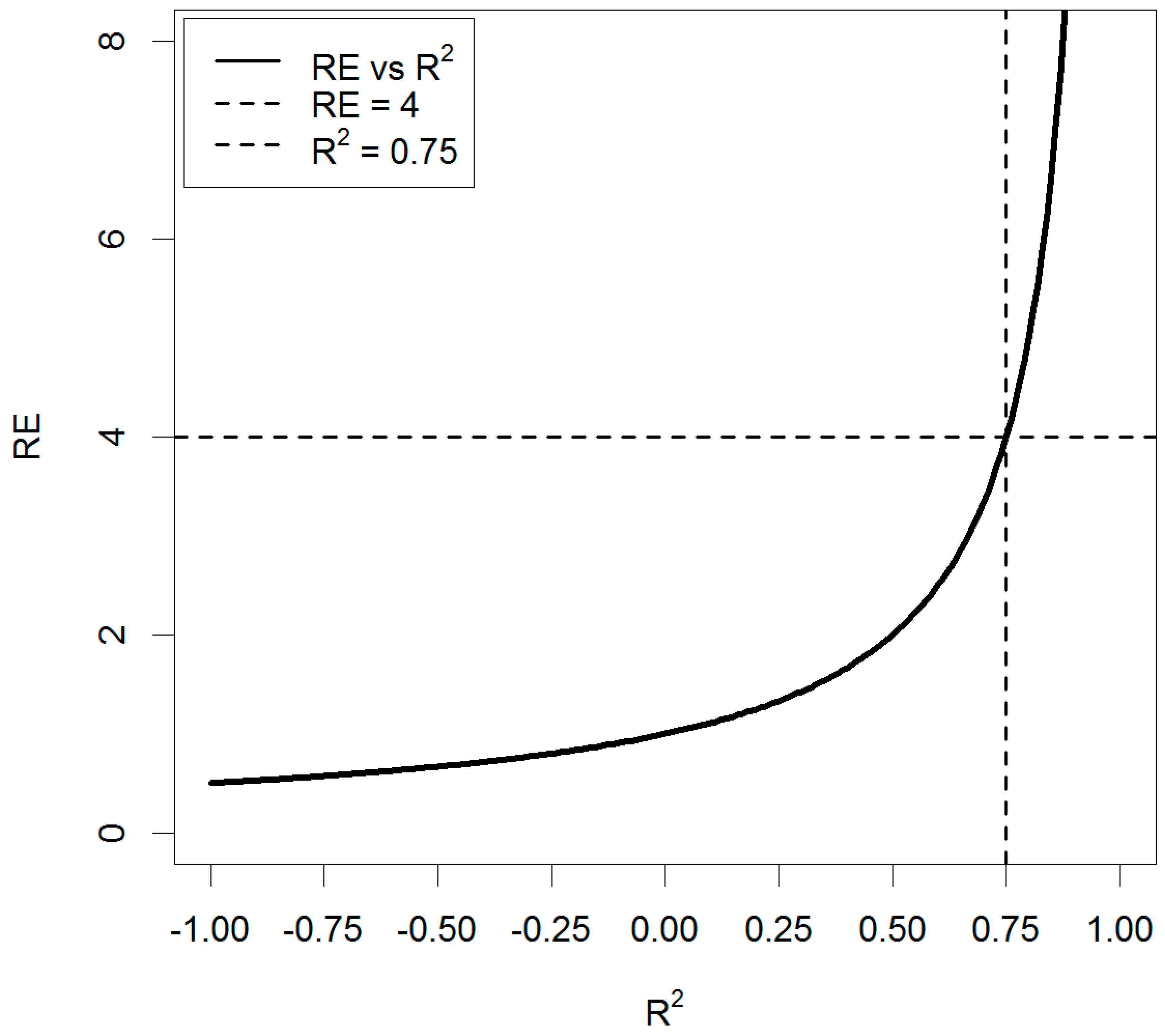
3.7. Efficiency Assessment

We evaluate performances in terms of efficiency for multiple estimation strategies where an “estimation strategy” consists of an estimator paired with a dataset. Efficiency is defined as the sampling variation for a given number of sample observations. An estimation strategy that is more efficient than another will have lower variance than another estimation strategy for the same number of observations, all other things being equal. There is not, however, a single way to measure or report efficiency.

In this study we primarily quantify efficiency with Relative Efficiency ($RE$). Relative efficiency, as defined here, is the estimated ratio of SRS mean variance without auxiliary information over the mean variance for an alternative estimator:

$$\begin{gathered} RE=\frac{v\left({\widehat{\mu }}_{SRS,n}\right)}{v\left({\widehat{\mu }}_{A,n}\right)} \\ v\left({\widehat{\mu }}_{A,n}\right)isthevarianceestimator forsomealternativedesign \end{gathered}$$

(12)

An advantage to using relative efficiency for inference is that it can be interpreted as a function of the sampling effort (e.g., the number of measured field plots). Relative efficiency is the estimated proportion of observations needed with ${\widehat{\mu }}_{SRS}$ to achieve the same precision as with ${\widehat{\mu }}_{A,n}$. For example, if a dataset has $RE$ = 2.0 for some alternative mean estimator ${\widehat{\mu }}_A$, then the variance estimated for ${\widehat{\mu }}_A$ with n plots is equivalent to the variance estimated for ${\widehat{\mu }}_{SRS}$ with $2\times n$ plots (${\widehat{\mu }}_{SRS}$ requires twice as many plots as ${\widehat{\mu }}_{A,n}$). This makes it possible to estimate the added value of ${\widehat{\mu }}_A$ in term of the cost required to measure additional plots with ${\widehat{\mu }}_{SRS}$ to be as precise as ${\widehat{\mu }}_{A,n}$. Our inferences rely largely on comparisons between the relative efficiencies of estimation strategies.

A common measure of statistical performance in modeling is the coefficient of determination ($R^2$) which can also be used to measure efficiency. The interpretation of $R^2$ is the (estimated) proportion of variation explained. Using the same notation as for relative efficiency, we define:

$$R^2=1-\frac{v\left({\widehat{\mu }}_{A,n}\right)}{v\left({\widehat{\mu }}_{SRS,n}\right)}.$$

(13)

From a sampling perspective, the main inference that can be drawn directly from $R^2$ values is that the estimation strategy with a higher $R^2$ value is more efficient than another strategy. Advantages of reporting R² include that it is commonly used in the literature related to area-based forest modeling with lidar (e.g., Reference [31]), its ease of interpretation, and its stability for high values of equivalent relative efficiencies.

As can be seen in Figure 5, relative efficiency and R² are closely related statistics and there is an exponential relationship between relative efficiency and R². While there are advantages to using relative efficiency for inference in a sampling context, the exponential behavior of relative efficiency can be a weakness when interpreting values on the order of 5 or greater. The issue is mitigated somewhat with a sufficiently large sample size (RE becomes more stable), or by simply recognizing that high relative efficiency values may be unstable and building some degree of caution into inferences.

4. Results

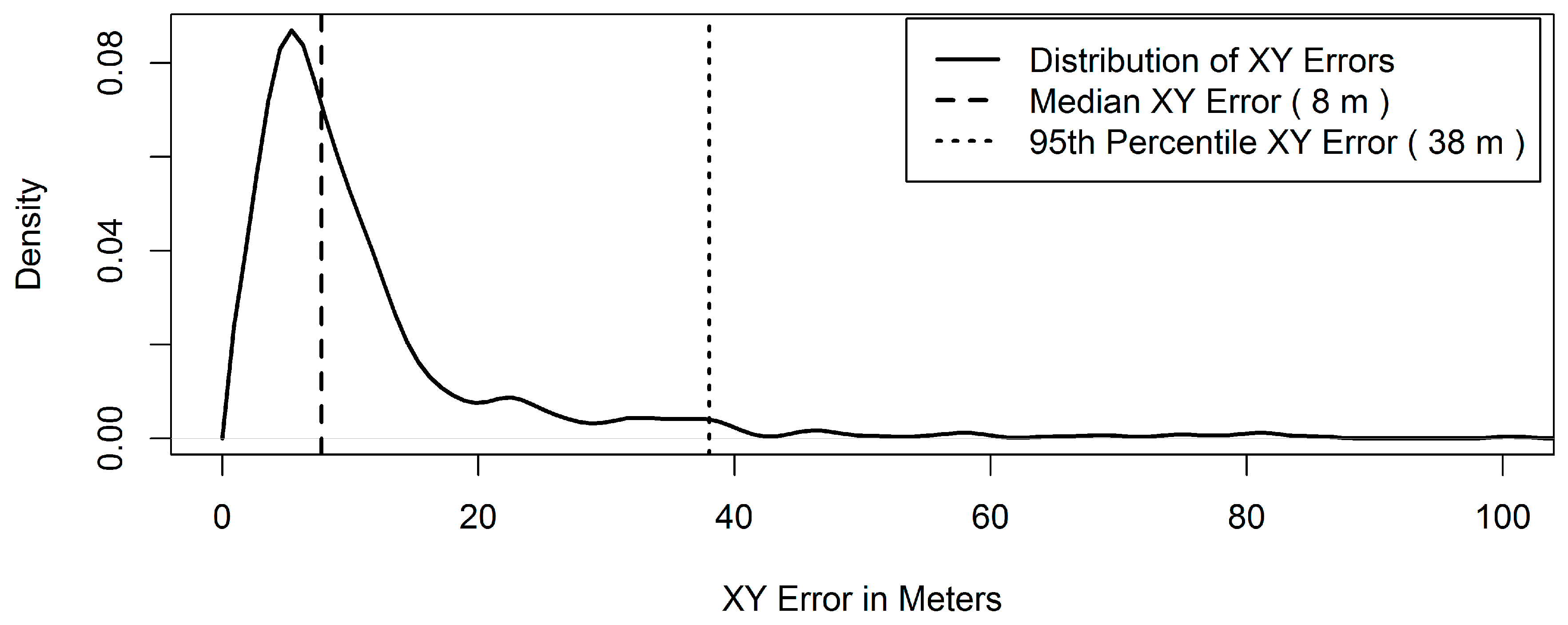
4.1. Coordinate Precision

One of the comparisons examined in this study is between estimation with HPL (High Precision Location) versus SPL (Standard Precision Location) coordinates. In Figure 6 we can see that positioning precision is a relevant concern, as 5% of observations appear to exceed 38 m in positioning error. For these plots, there would be no overlap between the remote sensing footprint and the location on the ground where field measurements were obtained. We investigate this issue further in later sections by looking at the impact of coordinate error on estimation. Substantial coordinate error may result in high variability between field and remotely-sensed forest structure measurements.

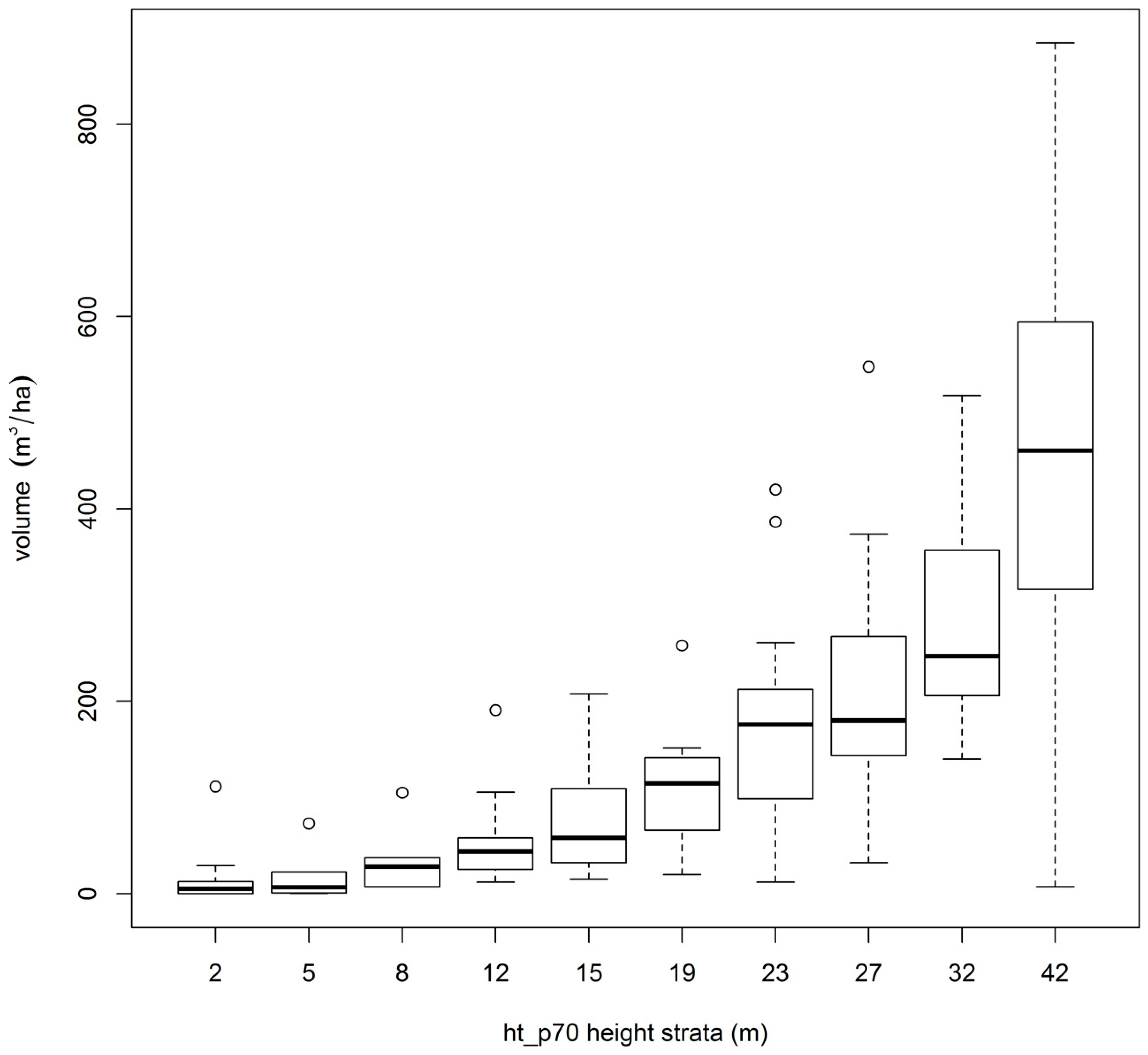
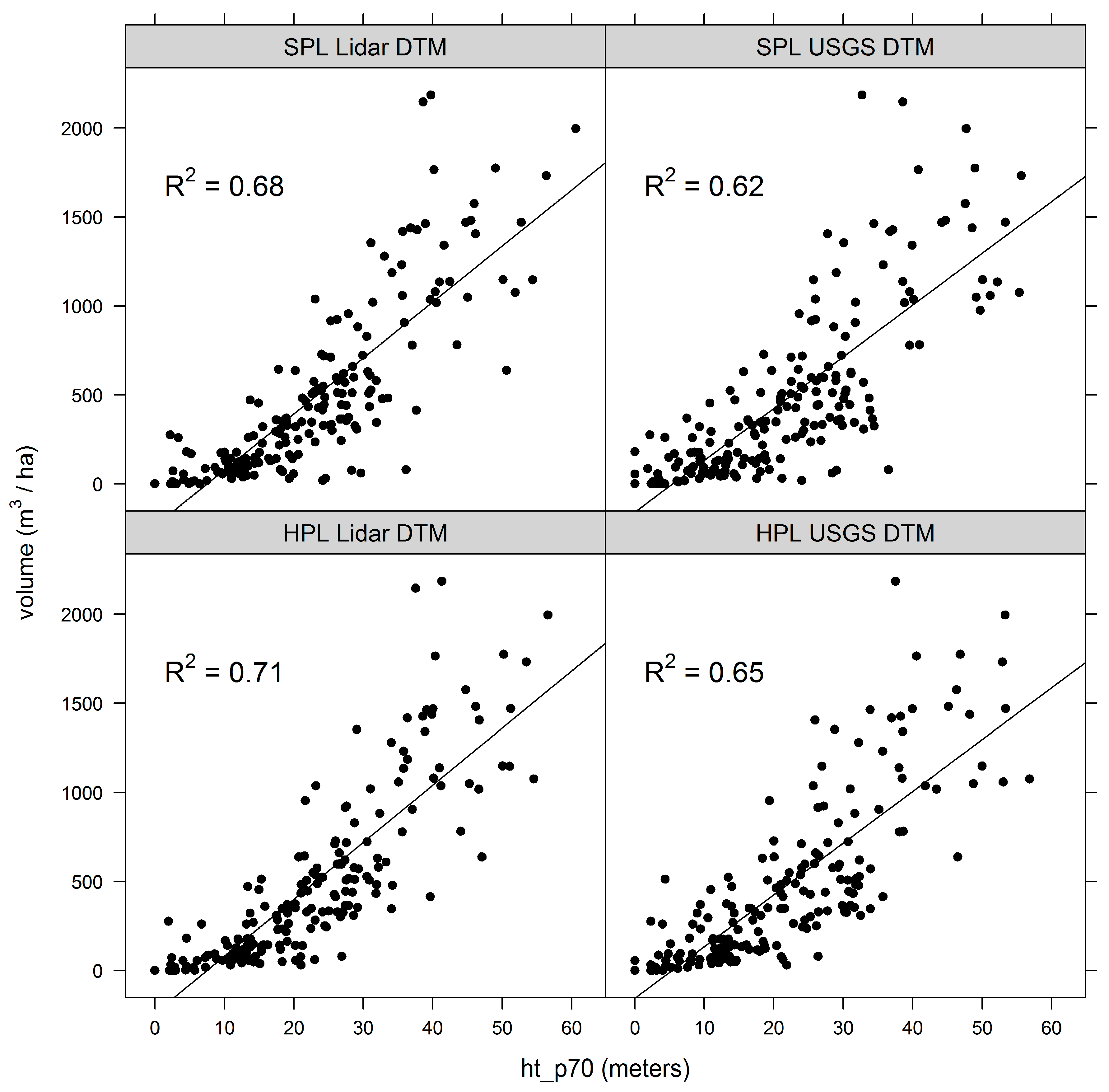
4.2. DAP Metrics versus Volume

Figure 7 shows the relationship between ht_p70 and volume for four scenarios including (1) HPL–USGS DTM (2) SPL–USGS DTM (3) HPL–lidar DTM (4) SPL–lidar DTM. The R² values in Figure 7 suggest that the association between volume and DAP height metrics is strongest for HPL with a lidar DTM, with the greatest reduction in performance resulting from using a USGS DTM, followed by using SPL coordinates. Although we can see that DTM source and coordinate quality have demonstrable impacts on the relationship between volume and height, even in the worst case (USGS DTM and SPL coordinates), there is still a strong relationship between the variables. Visually, the relationships and positions of points in the scatterplots appear very similar with only slight differences in spreads and in trends.

4.3. Increased Map Resolution with DAP

Figure 8 demonstrates one of the practical advantages of having high-resolution auxiliary height information to support forest yield estimation. When paired with precise, fine-resolution remote sensing, forest inventory measurements can be used to make precise, fine-resolution maps of forest attributes such as volume. FIA measurements without auxiliary height measurements support county-level estimates. In Figure 8, for example, Mason County (in green) would have a single estimate of total volume. The mapped product, in contrast, provides a very fine level of detail, describing the spatial distribution of volume within the county. While at times useful, it is important to note that aggregates (e.g., mean or sum) of mapped predictions are not design-unbiased for the stand, stratum, county, or any other tessellation of the population. Asymptotically unbiased estimation is feasible at the county level with the appropriate estimator, although biased synthetic estimates may be sufficient for some applications (e.g., Reference [32]).

4.4. Estimation Performance

Table 1. Measures of efficiency for various estimation strategies, n = 191 plots.

Estimator	Dataset	SE (m3/ha)	RE	R2
post-stratified	HPL lidar	22.60	4.16	0.76
post-stratified	SPL lidar	24.74	3.47	0.71
post-stratified	HPL USGS	24.38	3.57	0.72
post-stratified	SPL USGS	27.06	2.88	0.65
regression	HPL lidar	23.72	3.78	0.74
regression	SPL lidar	23.97	3.70	0.73
regression	HPL USGS	25.80	3.19	0.69
regression	SPL USGS	26.44	3.01	0.67

provides the efficiencies estimated for multiple estimation strategies. Standard error (SE) and R² values are also provided, although all of our inferences are based on RE. SE and R² values in Table 1 are present as a reference to enable comparisons with other studies. The difference in estimation strategies in Table 1 are based upon estimator (regression or post-stratified), type of plot positioning (HPL or SPL), and source of DTM (USGS or lidar). The results with respect to HPL plot locations and use of a lidar DTM are fairly intuitive. Both the lidar DTM and HPL were presumed to be higher quality data sources, which was confirmed when estimation with the lidar DTM and HPL coordinate data resulted in better relative efficiencies than the alternatives. For post-stratification, estimation with SPL caused the greatest singular reduction in efficiency. Estimation with a lidar DTM and HPL is equivalent to having 4.16 times as many plots as an SRS, but estimation with a lidar DTM and SPL is only equivalent to 3.47 times as many plots. Using SPL coordinates had the greatest impact on post-stratification, likely because even minor changes in height due to registration error could move a plot into an entirely different height stratum. The regression estimator was fairly insensitive to HPL versus SPL. The post-stratification approach was more sensitive to changes in estimation strategy: It yielded both the best result (HPL with a lidar DTM) and the worst result (SPL with a USGS DTM).

5. Discussion

5.1. Terrain Models

The results indicate that the best performance is achieved with a lidar DTM, although post-stratification on height with at USGS DTM is still 3.57 times as efficient as estimation without DAP heights. This agrees with results from another study which found that for a boreal forest, results using DAP based heights computed with a 10 m DTM compared well with using DAP with a lidar DTM [33]. We did not, however, explore what is the best way to incorporate two separate sources of DTMS into a single large-area remote sensing augmented forest inventory. Two approaches we considered include (1) mosaic lidar and USGS DTMs and give priority to the lidar DTMs, and (2) implement the inventory separately for areas with lidar and USGS DTMs. In the case of the second approach, this means fitting models separately for the two distinct data types, and then mosaicking results and estimates back together at the end. Metrics computed on lidar and USGS DTMs may be sufficiently different that the models may fit better in approach 2, although clearly this warrants further testing.

Another approach worth real consideration based upon the result observed here is implementation using only NED DEMs. This would be the simplest approach and would eliminate any edge artifacts that could arise due to differences between lidar and USGS DTMs. Clearly this would sacrifice a modicum of performance in areas with lidar DTMs and could be especially concerning for fine-resolution map products.

5.2. Positional Accuracy

Plot positioning under the canopy has proven to be a difficult endeavor over the history of forest measurements, and even today precise plot locations under canopy requires considerable investments in technology, planning, and GNSS data processing. Even predating the current HPL program, PNW FIA invested heavily in plot positioning, from having field crews attempt accurate pin-prick plot centers on orthophotos to using military-grade GPS equipment. As a result, the distribution of positional errors prior to HPL was actually encouraging. On average, 50% of plots were found to have better than 8 m error and 95% had better than 38 m of error (treating HPL coordinates as “correct”). However, these errors had a demonstrable effect on estimation performance, especially when using post-stratification.

The observed efficiencies for an area-based approach with SPL demonstrate one of the advantages of area-based inference over individual tree analysis approaches in the presence of positioning errors. While PNW has invested in precise plot locations on recent plot measurements, older recordings and other parts of the country do not have precise plot locations. Our results indicate that while performance will decline, plots with poor positioning accuracy can still be used with DAP to improve estimation. However, the observed SPL positing errors are too large to be expected to reliably align with individual trees.

Plot positioning errors (SPL) are sufficiently large that the plots with the worst errors likely contribute a large amount of noise. For example, the worst 5% of plot positions had positioning errors of 38 m or greater. The magnitude of errors observed in plot locations in Figure 7, and the demonstrated loss of estimation efficiency without HPL plot locations demonstrates the importance of HPL positioning to the implementation of remote sensing augmented forest inventory approaches. From this perspective, not having HPL may be equivalent to replacing 5% of observations with random noise, and commonly the worst plot positions fall in areas with the greatest topographic relief the largest trees, where forest types with the largest trees are commonly of the greatest interest.

5.3. Estimators

The best performance was observed for estimation with post-stratification, although it could not be deemed a clear “winner”. The regression estimator appeared to be more stable with respect to positioning errors, which would be advantageous for datasets for which HPL was not available. This makes sense because unlike post-stratification, a well-fit regression model on a continuous explanatory variable does not cause sharp changes in predictions for slight changes in the explanatory variable, which can happen with post-stratification when near the borders of the strata. That said, the magnitude of change between height bins is an artifact of the number of height bins, and for sufficient numbers of bins, regression and post-stratification would essentially converge. However, increasing the number of strata requires a sufficient number of observations to be able to reliably estimate strata means for a large number of height bins, something that will not always be feasible, but the point remains that we may be able to refine our approach to post-stratification to mitigate the sensitivity of the strategy to positioning errors. For example, it may help to post-stratify on predicted volume, or some other linear combination of our explanatory variables, further enmeshing the post-stratification and regression estimation as in References [29] and [34].

From a practical standpoint, post-stratification is much more convenient to implement than regression estimation. FIA already uses post-stratification to deal with forest/non-forest conditions and to adjust for non-response bias. From the FIA perspective, post-stratification could be a drop-in replacement or augmentation for the post-stratification that is already in place.

Regression estimation is more complex to implement and requires making a number of additional decisions. The best performance for a single attribute will be achieved by fitting each attribute separately, i.e., a separate linear regression model with a separate set of predictors. This tends to be unwieldy for an inventory program that estimates hundreds or thousands of attributes. The preferable alternative is to sacrifice slightly on performance and use the regression relationship to estimate a weight for each observation, and then apply the weight identically for all attributes. This approach to estimation is called regression calibration [35]. People have also turned to nearest neighbor algorithms to deal with simultaneously predicting large numbers of attributes from remote sensing [36]. Nearest neighbor approaches are convenient for managing the complexity of forest attributes, but there is currently limited documentation for implementation in a design-based framework. In practice the results (maps and estimates) are likely to be fairly similar between post-stratification and regression calibration, suggesting that, initially at least, post-stratification is preferable to incorporate remote sensing into estimation with FIA field measurements.

5.4. Comparison with Other Studies

Research studies which have evaluated lidar and DAP for forest inventory have tended to focus their inferences about performance on R² and RMSE instead of relative efficiency. The emphasis on residual variation is likely due in part to the prevalence of linear regression as a tool for inferential modeling and mapping, and the relative obscurity of sampling methods. In an exception that discussed efficiency directly [10], lidar was used to estimate volume in addition to biomass, basal area, and number of stems, and achieve a relative efficiency of 4.5 for volume (reported in the study as design effect, which is 1/RE), which is similar to the efficiencies observed in this study. It is fairly common for studies using lidar to exceed the R² values observed here. In this study we observed at best R² values of 0.76, where it is not unusual to see R² values which exceed 0.8 or even 0.9 for volume in the literature when using lidar-derived height attributes (e.g., References [37,38]), and values greater than 0.75 for frame-based DAP (e.g., References [12,13,14]).

Our findings with respect to the effects of using SPL versus HPL on efficiency are similar to what was observed in another study [39]. The related study examined the effects of up to 6m in positional error on lidar based regression predictions of aboveground biomass for multiple plot sizes. For the plot size most similar to the area of an FIA plot (707 m² in the related study versus 675 m² for an FIA plot [39] the effect of 6m positional errors on R² values was on the order of a 2–3 percent, or roughly the same as the difference in R² values that we observed between HPL and SPL coordinates with a regression estimator.

The relative efficiencies observed in this study for post-stratification are comparable to those found for post-stratification of volume using auxiliary lidar heights in Reference [34]. This study differs from Reference [34] in that we used more strata (10 versus 6), and we stratified on a single auxiliary variable. Our finding that the relative efficiencies of post-stratification and model-assisted estimation agrees with another study [40], although our studies used different sources of auxiliary information (DAP versus NLCD [41]). Two other studies, References [29] and [28], disagreed with our findings and found that model-assisted estimation was more efficient than post-stratification. Key distinctions between this study and References [29] and [28] include that the method we used only measured data and post-stratified on a single auxiliary variable where they used simulated data and looked a post-stratification using combinations of multiple auxiliary variables. We are uncertain as to the root cause of our different findings, but they may be attributable to these differences in data and methodology.

5.5. Feasibility

A driving motivation to pursue alternatives to lidar to explain vertical forest structure is that lidar is very expensive. We envision DAP as a lower-cost technology which can also provide forest height. Point clouds derived from DAP are typically much less expensive than lidar, even if it is necessary to collect new imagery to support the effort. For example, new imagery and an associated point cloud may cost on the order of $0.3 USD per hectare, and less than $0.01 per hectare if the imagery has already been flown and the vendor has historical imagery in their archive. Area-wide DAP for Washington State (186k km²) can be obtained for under $200k USD when derived from existing imagery. At this kind of pricing, frequent, high-precision, high-resolution forest inventory becomes more readily feasible.

5.6. Monetary Value of Efficiency

A practical implication of increased relative efficiency with DAP is that it is feasible to achieve higher estimation precision for the same number of plots. For a large area, e.g., all of Washington State, the effect may not be very impactful, but for sub-regions such as a single county, it can mean the difference between usable and unusable forest yield estimates. For sub-region estimates without auxiliary information, a small number of plots within the region may result in unreliable estimates. Integration of remote sensing information with field measured plot data for estimation is equivalent to having additional plots (for attributes related to height and cover). Here we briefly quantify the added monetary value of DAP when performing an estimation with FIA field plots using some simplifying assumptions. A major caveat to this exercise is that DAP provides little or no explanatory power for many field-measured forest attributes. For these attributes, DAP provides no added value, and it can prove difficult to untangle added value when some estimates are improved by DAP and others are not.

The use of a permanent grid of field plots is fairly standard practice and individual plot costs can be fairly high (100’s to 1000’s of dollars), often because of the high cost of travel between plots (and often because lots of kinds of measurements are taken on permanent plots). For this exercise, we will assume that the majority of the value of the plot is associated with forest attributes which can easily be related to remotely measured height, attributes such as height [42], basal area [43], volume [44], biomass [42], and carbon [8]. For the sake of simplicity we will assume that the hypothetical cost per plot is $1000 for some inventory (actual FIA plot costs in WA vary greatly but are expected to be $\approx \$2000$/plot on average), that our area of interest has 100 field measurement plots, and that the values in Table 1 are applicable. Based on our results in Table 1, our estimation strategies with auxiliary DAP ranged from 3–4 times as efficient as estimation without DAP (assuming SRS). In the case of our area with 100 field plots, this is equivalent to having 3–4 times as many plots or an additional 200–300 plots. With our assumption of $1000/plot, this is an added value of $200,000–$300,000, a substantial increase.

This same approach can be used to quantify the value associated with differences amongst the estimation strategies that we presented in Table 1. In the case of post-stratification with HPL versus SPL, there is a 0.7 unit difference in relative efficiency. For our same target area with 100 plots, this is equivalent to having $0.7\times 100$ = 70 additional plots, or an added value of $70,000 at $1000/plot. If we divide this added value amongst the existing 100 plots in the county, HPL provides an added value of $\$\mathrm{70,000} ÷100=\$700$ per plot. Based on the provided assumptions, as long as the added cost of HPL does not exceed $700/plot, the HPL program adds value to the inventory.

5.7. Scope of Inference

Estimates in this study use data that are restricted to the extent of the lidar DTM. As a result, our inferences are only about the relative performances of estimation strategies, and do not represent point estimates for all of Washington State. The tables of results provided in this study are only appropriate to guide the selection of an estimation strategy, not as stand-alone values.

5.8. Study Limitations and Future Direction

This study focuses on attributes and measurements which are associated with forest structure. Forest inventory crews typically measure a wide variety of forest attributes, many of which cannot be easily modeled from remotely-sensed forest structure measurements. This oversight (not explicitly addressing other forest attributes) is especially apparent when we monetize the added value of upgrading our inventory with remote sensing. The added value is only applicable to attributes for which remote sensing can aid in estimation, and in our toy example we assign the full value of an additional plot ($1000) to the added efficiency, whereas some of that value is in fact lost due to the fact that remote sensing was not used to aid in (e.g.,) estimation of species proportions. In practice, consideration must be given to the fact that many of the attributes which are not easily captured with height-based measurements are also important for a wide variety of important inferences about our nation’s forest. Most forest inventory applications are dependent on measurements such as species and damage which are not easily accounted for by the approach used here.

In some instances, estimates for difficult to measure attributes (with remote sensing) can still see some improvement when combined with height-related attributes. Biomass by species (e.g.,) will not have improvement in the species proportion component of the estimate, but the biomass component of the estimate is improved, which can result in a lower average error for biomass by species.

Future research efforts will include investigation of a greater variety of forest attributes, and integration with additional sources of information such as weather, elevation, and spectral information (especially Landsat time series), which may aid in the modeling and estimation of a wider variety of forest attributes.

6. Conclusions

This study demonstrates that pushbroom imagery (DAP) can be used to increase both the efficiency and resolution of forest yield estimates. While high-resolution area-wide height measurements have been available from lidar for some time, low-cost pushbroom DAP makes for a compelling case for wide-scale and repeated acquisitions to support forest yield mapping and estimation. The maturation of this technology provides incredible new opportunities to examine vegetative structure such as height, biomass, and volume for entire states at a level of precision and resolution that typically are only available for the extents of relatively small and infrequent lidar projects. One could imagine, for example, that state-wide fine-resolution maps of canopy fuel model parameters such as crown bulk density could prove advantageous for planning and risk assessment in the current era of increasing fire size and severity. For the few exceptions where states have complete lidar coverage, these states are ideally situated to leverage lidar DTMs with frequent low-cost statewide DAP acquisitions.

References

- Smith, W.B. Forest inventory and analysis: A national inventory and monitoring program. Environ. Pollut. 2002, 116, S233–S242. [Google Scholar] [CrossRef]
- The Enhanced Forest Inventory and Analysis Program: National Sampling Design and Estimation Procedures; Bechtold, W.A.; Patterson, P.L. (Eds.) US Department of Agriculture Forest Service, Southern Research Station: Asheville, NC, USA, 2005.
- Blackard, J.A.; Finco, M.V.; Helmer, E.H.; Holden, G.R.; Hoppus, M.L.; Jacobs, D.M.; Lister, A.J.; Moisen, G.G.; Nelson, M.D.; Riemann, R.; et al. Mapping U.S. forest biomass using nationwide forest inventory data and moderate resolution information. Remote Sens. Environ. 2008, 112, 1658–1677. [Google Scholar] [CrossRef]
- Waring, R.H.; Coops, N.C.; Fan, W.; Nightingale, J.M. MODIS enhanced vegetation index predicts tree species richness across forested ecoregions in the contiguous U.S.A. Remote Sens. Environ. 2006, 103, 218–226. [Google Scholar] [CrossRef]
- Næsset, E. Determination of mean tree height of forest stands using airborne laser scanner data. ISPRS J. Photogramm. Remote Sens. 1997, 52, 49–56. [Google Scholar] [CrossRef]
- Holmgren, J. Prediction of tree height, basal area and stem volume in forest stands using airborne laser scanning. Scand. J. For. Res. 2004, 19, 543–553. [Google Scholar] [CrossRef]
- Anderson, H.E.; Breidenbach, J. Statistical Properties of Mean Stand Biomass Estimators in a Lidar-Based Double Sampling Forest Survey Design; International Society for Photogrammetry and Remote Sensing: Istanbul, Turkey, 2007; p. 8. [Google Scholar]
- Patenaude, G.; Hill, R.A.; Milne, R.; Gaveau, D.L.A.; Briggs, B.B.J.; Dawson, T.P. Quantifying forest above ground carbon content using LiDAR remote sensing. Remote Sens. Environ. 2004, 93, 368–380. [Google Scholar] [CrossRef]
- Andersen, H.-E.; McGaughey, R.J.; Reutebuch, S.E. Estimating forest canopy fuel parameters using LIDAR data. Remote Sens. Environ. 2005, 94, 441–449. [Google Scholar] [CrossRef]
- Strunk, J.L.; Reutebuch, S.E.; Andersen, H.-E.; Gould, P.J.; McGaughey, R.J. Model-assisted forest yield estimation with light detection and ranging. West. J. Appl. For. 2012, 27, 53–59. [Google Scholar] [CrossRef]
- Sugarbaker, L.J.; Eldridge, D.F.; Jason, A.L.; Lukas, V.; Saghy, D.L.; Stoker, J.M.; Thunen, D.R. Status of the 3D Elevation Program, 2015; US Geological Survey: Reston, VA, USA, 2017.
- White, J.C.; Stepper, C.; Tompalski, P.; Coops, N.C.; Wulder, M.A. Comparing ALS and image-based point cloud metrics and modelled forest inventory attributes in a complex coastal forest environment. Forests 2015, 6, 3704–3732. [Google Scholar] [CrossRef]
- Bohlin, J.; Wallerman, J.; Fransson, J.E.S. Forest variable estimation using photogrammetric matching of digital aerial images in combination with a high-resolution DEM. Scand. J. For. Res. 2012, 27, 692–699. [Google Scholar] [CrossRef]
- Vastaranta, M.; Wulder, M.A.; White, J.C.; Pekkarinen, A.; Tuominen, S.; Ginzler, C.; Kankare, V.; Holopainen, M.; Hyyppä, J.; Hyyppä, H. Airborne laser scanning and digital stereo imagery measures of forest structure: comparative results and implications to forest mapping and inventory update. Can. J. Remote Sens. 2013, 39, 382–395. [Google Scholar] [CrossRef]
- National Elevation Dataset (NED) | The Long Term Archive. Available online: https://lta.cr.usgs.gov/NED (accessed on 7 August 2018).
- Gesch, D.B.; Oimoen, M.J.; Evans, G.A. Accuracy Assessment of the US Geological Survey National Elevation Dataset, and Comparison with Other Large-area Elevation Datasets: SRTM and ASTER; US Geological Survey: Reston, VA, USA, 2014.
- US Department of Commerce. National Geodetic Survey—CORS Homepage. Available online: https://www.ngs.noaa.gov/CORS/ (accessed on 2 October 2018).
- McGaughey, R.J.; Ahmed, K.; Andersen, H.-E.; Reutebuch, S.E. Effect of Occupation Time on the Horizontal Accuracy of a Mapping-Grade GNSS Receiver under Dense Forest Canopy. Photogramm. Eng. Remote Sens. 2017, 83, 861–868. [Google Scholar] [CrossRef]
- NAIP Imagery. Available online: https://www.fsa.usda.gov/programs-and-services/aerial-photography/imagery-programs/naip-imagery/ (accessed on 12 March 2019).
- Isenburg, M. LASzip: lossless compression of LiDAR data. Photogramm. Eng. Remote Sens. 2013, 79, 209–217. [Google Scholar] [CrossRef]
- Davis, D. NAIP Accuracy and Ground Control Point Collections 2016. Available online: https://www.fgdc.gov/groups/naip-accuracy-and-gcps-20160804.pptx (accessed on 5 February 2019).
- McGaughey, R.J. FUSION/LDV: Software for LIDAR Data Analysis and Visualization, Version 3.01; USFS: Seattle, WA, USA, 2016.
- Washington Lidar Portal. Available online: http://lidarportal.dnr.wa.gov/ (accessed on 6 March 2019).
- Särndal, C.E.; Swensson, B.; Wretman, J. Model Assisted Survey Sampling; Springer Verlag: New York, NY, USA, 2003. [Google Scholar]
- Cochran, W.G. Sampling Techniques, 3rd ed.; John Wiley & Sons: New York, NY, USA, 1977; ISBN 0-471-16240-X. [Google Scholar]
- Goerndt, M.E.; Monleon, V.J.; Temesgen, H. Small-Area Estimation of County-Level Forest Attributes Using Ground Data and Remote Sensed Auxiliary Information. For. Sci. 2013, 59, 536–548. [Google Scholar] [CrossRef]
- Furnival, G.M.; Wilson, R.W., Jr. Regressions by leaps and bounds. Technometrics 1974, 16, 499–511. [Google Scholar] [CrossRef]
- Myllymäki, M.; Gobakken, T.; Næsset, E.; Kangas, A. The efficiency of poststratification compared with model-assisted estimation. Can. J. For. Res. 2016, 47, 515–526. [Google Scholar] [CrossRef]
- Magnussen, S.; Andersen, H.-E.; Mundhenk, P. A Second Look at Endogenous Poststratification. For. Sci. 2015, 61, 624–634. [Google Scholar] [CrossRef]
- Breidt, F.J.; Opsomer, J.D. Endogenous post-stratification in surveys: Classifying with a sample-fitted model. Ann. Stat. 2008, 36, 403–427. [Google Scholar] [CrossRef]
- Pearse, G.D.; Dash, J.P.; Persson, H.J.; Watt, M.S. Comparison of high-density LiDAR and satellite photogrammetry for forest inventory. ISPRS J. Photogramm. Remote Sens. 2018, 142, 257–267. [Google Scholar] [CrossRef]
- D’Oliveira, M.V.; Reutebuch, S.E.; McGaughey, R.J.; Andersen, H.-E. Estimating forest biomass and identifying low-intensity logging areas using airborne scanning lidar in Antimary State Forest, Acre State, Western Brazilian Amazon. Remote Sens. Environ. 2012, 124, 479–491. [Google Scholar] [CrossRef]
- Kukkonen, M.; Maltamo, M.; Packalen, P. Image matching as a data source for forest inventory—Comparison of Semi-Global Matching and Next-Generation Automatic Terrain Extraction algorithms in a typical managed boreal forest environment. Int. J. Appl. Earth Obs. Geoinf. 2017, 60, 11–21. [Google Scholar] [CrossRef]
- McRoberts, R.E.; Gobakken, T.; Næsset, E. Post-stratified estimation of forest area and growing stock volume using lidar-based stratifications. Remote Sens. Environ. 2012, 125, 157–166. [Google Scholar] [CrossRef]
- Särndal, C.E. The calibration approach in survey theory and practice. Surv. Methodol. 2007, 33, 99–119. [Google Scholar]
- Packalén, P.; Maltamo, M. Estimation of species-specific diameter distributions using airborne laser scanning and aerial photographs. Can. J. For. Res. 2008, 38, 1750–1760. [Google Scholar] [CrossRef]
- Means, J.E.; Acker, S.A.; Fitt, B.J.; Renslow, M.; Emerson, L.; Hendrix, C. Predicting Forest Stand Characteristics with Airborne Scanning Lidar. Photogramm. Eng. Remote Sens. 2000, 66, 1367–1371. [Google Scholar]
- Popescu, S.C.; Wynne, R.H.; Scrivani, J.A. Fusion of Small-Footprint Lidar and Multispectral Data to Estimate Plot- Level Volume and Biomass in Deciduous and Pine Forests in Virginia, USA. For. Sci. 2004, 50, 551–565. [Google Scholar]
- Frazer, G.W.; Magnussen, S.; Wulder, M.A.; Niemann, K.O. Simulated impact of sample plot size and co-registration error on the accuracy and uncertainty of LiDAR-derived estimates of forest stand biomass. Remote Sens. Environ. 2011, 115, 636–649. [Google Scholar] [CrossRef]
- McRoberts, R.E.; Liknes, G.C.; Domke, G.M. Using a remote sensing-based, percent tree cover map to enhance forest inventory estimation. For. Ecol. Manag. 2014, 331, 12–18. [Google Scholar] [CrossRef]
- Yang, L.; Jin, S.; Danielson, P.; Homer, C.; Gass, L.; Bender, S.M.; Case, A.; Costello, C.; Dewitz, J.; Fry, J.; et al. A new generation of the United States National Land Cover Database: Requirements, research priorities, design, and implementation strategies. ISPRS J. Photogramm. Remote Sens. 2018, 146, 108–123. [Google Scholar] [CrossRef]
- St-Onge, B.; Hu, Y.; Vega, C. Mapping the height and above-ground biomass of a mixed forest using lidar and stereo Ikonos images. Int. J. Remote Sens. 2008, 29, 1277–1294. [Google Scholar] [CrossRef]
- Gobakken, T.; Næsset, E. Estimation of diameter and basal area distributions in coniferous forest by means of airborne laser scanner data. Scand. J. For. Res. 2004, 19, 529–542. [Google Scholar] [CrossRef]
- Hawryło, P.; Tompalski, P.; Wężyk, P. Area-based estimation of growing stock volume in Scots pine stands using ALS and airborne image-based point clouds. For. Int. J. For. Res. 2017, 90, 686–696. [Google Scholar] [CrossRef]
- Available online: http://www.asprs.org/a/society/about.html (accessed on 21 August 2018).