Article

Assessing Hydrological Ecosystem Services in a Rubber-Dominated Watershed under Scenarios of Land Use and Climate Change

Institute of Agricultural Sciences in the Tropics and Subtropics (Hans-Ruthenberg-Institute), University of Hohenheim, 70593 Stuttgart, Germany
*
Author to whom correspondence should be addressed.
Forests 2019, 10(2), 176; https://doi.org/10.3390/f10020176
Submission received: 30 December 2018 / Revised: 7 February 2019 / Accepted: 15 February 2019 / Published: 19 February 2019

Abstract

:
Land use and climate change exert pressure on ecosystems and threaten the sustainable supply of ecosystem services (ESS). In Southeast-Asia, the shift from swidden farming to permanent cash crop systems has led to a wide range of impacts on ESS. Our study area, the Nabanhe Reserve in Yunnan province (PR China), saw the loss of extensive forest areas and the expansion of rubber (Hevea brasiliensis Müll. Arg.) plantations. In this study, we model water yield and sediment export for a rubber-dominated watershed under multiple scenarios of land use and climate change in order to assess how both drivers influence the supply of these ESS. For this we use three stakeholder-validated land use scenarios, varying in their degree of rubber expansion and land management rules. As projected climate change varies remarkably between different climate models, we combined the land use scenarios with datasets of temperature and precipitation changes, derived from nine General Circulation Models (GCMs) of the Fifth Assessment Report of the IPCC (Intergovernmental Panel on Climate Change) in order to model water yield and sediment export with InVEST (Integrated Valuation of Ecosystem Services and Trade-offs). Simulation results show that the effect of land use and land management decisions on water yield in Nabanhe Reserve are relatively minor (4% difference in water yield between land use scenarios), when compared to the effects that future climate change will exert on water yield (up to 15% increase or 13% decrease in water yield compared to the baseline climate). Changes in sediment export were more sensitive to land use change (15% increase or 64% decrease) in comparison to the effects of climate change (up to 10% increase). We conclude that in the future, particularly dry years may have a more pronounced effect on the water balance as the higher potential evapotranspiration increases the probability for periods of water scarcity, especially in the dry season. The method we applied can easily be transferred to regions facing comparable land use situations, as InVEST and the IPCC data are freely available.

1. Introduction

Ecosystem services (ESS) are defined as the goods and benefits humans gain from healthy and functional ecosystems [1]. Global change processes such as large-scale land use change and climate change increase pressure on ecosystem functions and threaten the sustainable supply of ESS [2,3,4,5]. In the last decades, the ESS concept has been increasingly used in environmental policy formulation and decision-making processes [6]. High impact publications such as the MEA (Millennium Ecosystem Assessment) [1] and TEEB (The Economics of Ecosystems and Biodiversity) [7] paved the way for the establishment of IPBES (Intergovernmental Platform on Biodiversity and Ecosystem Services) [8], who recently reported extensive land degradation and declining trends for many ESS and biodiversity all over the globe [9]. Several pathways exist for safeguarding the sustainability of future ESS supply. Modeling and mapping ESS for future scenarios of global change is one way to project the impact of land use or climate change on ESS in a spatially explicit manner [10]. Several tools are available to model ESS and how their future provision might be altered under scenarios of climate or land use change. Two of the most-used models are SWAT (Soil and Water Assessment Tool) [11] and InVEST (Integrated Valuation of Ecosystem Services and Trade-Offs) [12], which are most prominently used in the field of water-, soil- and climate-related ESS research [13]. Output of such modeling efforts can assist land use planners and policy makers and serve as a basis for the development of mitigation and adaptation strategies.
Global surface temperature and the variability of precipitation patterns in both time and space are highly likely to change over the course of the next century [14,15,16]. The Fifth Assessment Report of the Intergovernmental Panel on Climate Change (IPCC5) [17] provided multiple future trajectories of Relative Concentration Pathways (RCPs), in which the atmospheric concentration of gases relevant for Earth’s climate changes as a result of global-scale socio-economic decisions over the course of the next century. In general, global mean temperature is expected to increase in all RCPs, as the climate system responds with some delay to past changes in atmospheric greenhouse gas concentrations. Regional differences in temperature and precipitation vary in the amount (and direction) of projected changes as a result of the differences in the assumptions, resolutions, and parameterizations of General Circulation Models (GCMs). For this reason, mean results of ensemble model projections are often considered as the best estimate for future conditions in the field of climate research.
In montane mainland Southeast-Asia, the recent shift from traditional swidden farming to permanent cash crop systems has led to a wide range of impacts on ESS [18,19]. In Yunnan Province in Southwest China in particular, large areas of forest have been replaced by rubber (Hevea brasiliensis Müll. Arg.) plantations due to increasing rubber-based product demands [20,21,22]. Such extensive changes of land use can strongly affect multiple ESS [23,24]. Effects on hydrological ESS are of major concern, as land use changes influence many hydrological factors such as the interception of precipitation, run-off, sediment transport, and evapotranspiration. Hydrological effects of the expansion of rubber plantations range from increases in surface run-off and soil erosion [25,26], to increases in water loss via evapotranspiration in the dry season, and a reduction of water storage in the subsurface soil [27].
Other authors have estimated potential hydrological effects of climate change in montane mainland Southeast-Asia. Eastham et al. [28] showed potential increases in both mean annual temperature and precipitation in Yunnan Province and the rest of the Mekong basin. Studies on hydrology in the Mekong Region have shown potential impacts of climate change on streamflow, soil erosion rates, and sediment fluxes [29]. Zhu et al. [30] estimated increases in sediment fluxes in a catchment of the Upper Yangtze River as a response of changes in precipitation and temperature. Similar increases in both mean annual streamflow and sediment export have been estimated by Phan et al. [31] for the Song Cau watershed in Northern Vietnam.
However, only few studies included both land use change and climate change scenarios in their estimates for future ESS supply [32]. Trisurat et al. [33] used InVEST in combination with input data of (1) 10-year average precipitation (2000–2010), (2) precipitation predictions of one GCM for 2020, and (3) extreme precipitation (wet year of 2000) in combination with three land use scenarios. They found the highest water yield and sediment export for intensified land use with extreme precipitation conditions. Hoyer & Chang [32] applied InVEST using three GCMs for precipitation and temperature input data in order to represent a low, medium, and high range of potential climate paths. As the projected climate change varies substantially between different climate models, this uncertainty needs to be taken into account for watershed management and climate change adaptation [29].
In this study, we model two indicators for ESS—water yield and sediment export—for a rubber-dominated watershed under multiple scenarios of land use and climate change in order to assess how both drivers influence the supply of these ESS. For this purpose, we use spatially explicit data derived from nine General Circulation Models (temperature and precipitation) in combination with stakeholder-validated land use scenarios as input for a well-tested ESS modeling framework (InVEST). This study represents the first ESS assessment combining land use scenarios and multiple climate scenarios for rubber cultivation systems.

2. Materials and Methods

2.1. Study Area

The study area was the Naban River Watershed National Nature Reserve, which is referred to as the Nabanhe Reserve henceforth. It is located in Yunnan Province, Xishuangbanna Prefecture in the Peoples Republic of China (22°08′ N 100°41′ E). It covers an area of roughly 271 km² and its topography is characterized by sloping hills, with altitudes ranging from about 500 to 2300 meters above sea level (m.a.s.l.). Depending on elevation, mean annual temperature is 18–22 °C and annual average precipitation varies between 1100 and 1600 mm [26]. The region is characterized by a subtropical climate and is influenced by monsoon cycles. The wet season lasts from May to October and about 87% of the annual precipitation occurs within these months [34]. The region is located within the Indo-Burma biodiversity hotspot and features an exceptional species richness [35]. As the study area is located on the northernmost border of tropical Asia, it features a mixture of tropical and temperate florae, which are diversified in their distribution by the mountainous topography [36]. Natural or semi-natural tropical mountainous rainforests represent the largest part of Nabanhe Reserve and cover about 60% of its area. Agricultural land use systems present in the Reserve include paddy rice fields and other annual crops (e.g., maize), as well as perennial systems such as tea, banana, and rubber plantations. More details on land cover in Nabanhe Reserve are listed in Table 1. We chose Nabanhe Reserve because it encompasses a watershed with rubber plantations as the dominant land use, but also features extensive protected areas, as it is part of the UNESCO (United Nations Educational, Scientific and Cultural Organization) Man and the Biosphere Programme [37]. Rubber cultivation had been present in the region’s valley bottoms for decades, but has increasingly spread into the hillsides, where the rubber trees most commonly replace natural or semi-natural tropical mountainous rainforest [38]. The economic lifespan of rubber plantations in this area is around 20–25 years. Trees are commonly planted in monoculture on terraces in rows with about 3–4 m distance, whereas the distance between two adjacent terraces is about 5–7 m. Tree density ranges between 450 and 600 trees per hectare. Ground cover is kept low by the farmers, usually with two herbicide applications per year.

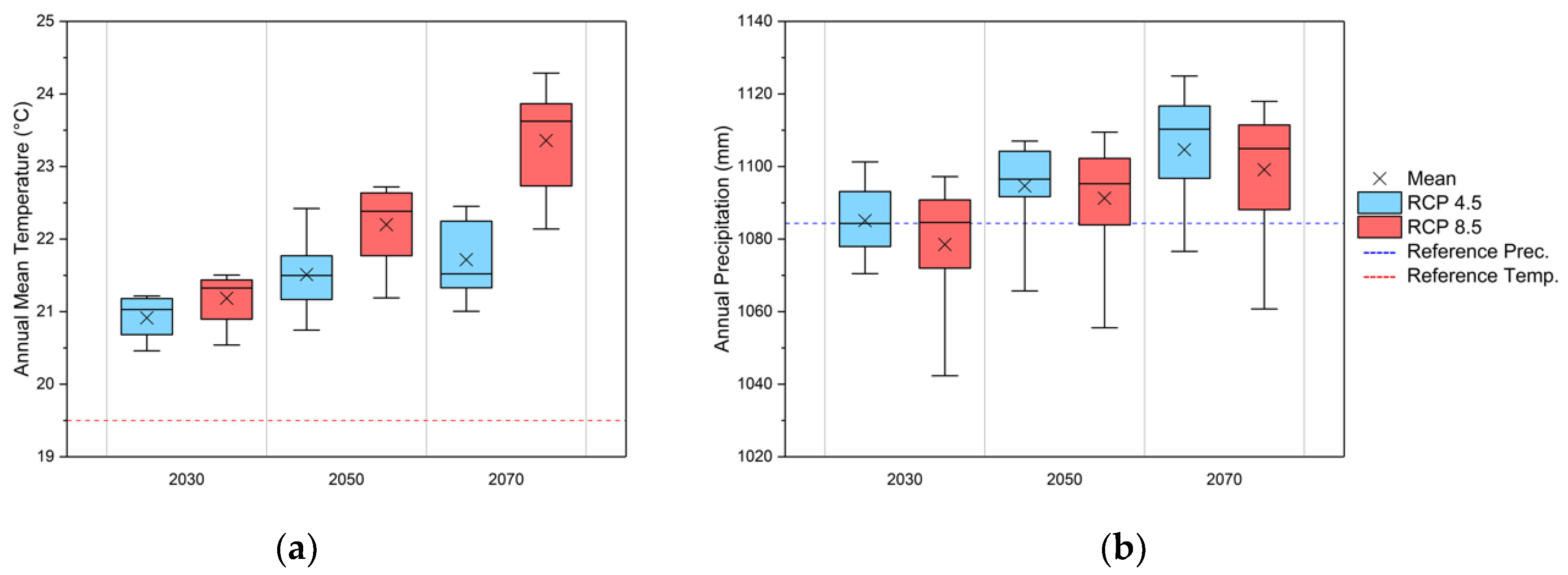
2.2. Climate Change Scenarios

InVEST was designed to be used with long-term average annual precipitation input data. We used the WorldClim dataset (Version 1.4) as baseline data, as it represents average annual precipitation derived from long-term measurements, which were interpolated to local topographical conditions [39,40]. We used precipitation and temperature data of nine GCMs and two RCPs (RCP 4.5 and RCP 8.5) as input for InVEST. RCP 4.5 is a moderate climate scenario which features a stabilization of greenhouse gas concentration by the year 2070 [41]. RCP 8.5 is a high emission scenario leading to an increase of 4 °C in global mean temperature by the end of the century in comparison to the pre-industrial era [42]. The GCMs were chosen based on their regional performance [43] according to the selection criteria of McSweeney et al. [44]. The output of the following GCMs was used: ACCESS1.0 [45,46], BCC_CSM1.1 [47], CCSM4 [48], GFDL CM3 [49], HadGEM2-ES [50], IPSL-CM5A-LR [51], MRI-CGCM3 [52], MPI-ESM-LR [53], and NorESM1-M [54]. Both temperature and precipitation datasets were obtained online at the “Climate Change Agriculture and Food Security-GCM Downscaled Data Portal” [55]. The geo-datasets were downloaded in ASCII-format and feature a horizontal resolution of roughly 900x900 m at the latitude of Xishuangbanna. We used ArcGIS (Version 10.3.1, [56]) to clip the geo-datasets to the extent of our study area, convert them to TIFF-format and project the data from “GCS_WGS_1984” to “WGS_1984_UTM_zone_47N” in order to match the grid of the rest of our spatial input data. The data is structured in three time slices centered around 2030 (2020–2040), 2050 (2040–2060) and 2070 (2060–2080) and includes annual average precipitation as well as monthly minimum, mean, and maximum temperature. Figure 1 depicts annual mean temperature (a) and annual precipitation (b) averaged over Nabanhe Reserve from the nine GCMs as well as baseline temperature and precipitation (WorldClim v1.4).
In addition to annual precipitation, InVEST requires annual potential evapotranspiration (PETa) as a spatially explicit input layer. In order to calculate PETa (mm/year) for each time slice of the climate change scenarios we used the output of the GCMs for monthly mean temperature (Tmean in °C) and daily temperature range (TD in °C, maximum temperature − minimum temperature). Extraterrestrial radiation (RA, radiation at the top of the atmosphere in mm/month as equivalent of evaporation) was obtained online from the “CGIAR-CSI Global Aridity and PET Database” [57,58,59]. We did not assume changes in RA during the course of the climate scenarios, so the geo-dataset of RA remained constant for each time slice. We used Hargreaves method [60] to calculate PETm (mm/month):
P E T m = 0.0023 × R A × ( T m e a n + 17.8 ) × T D 0.5 .
We calculated PETa by summing each cell of the monthly PET layers:
P E T a = m = 1 12 P E T m .
Hargreaves method [60] was chosen in order to keep consistency with previous InVEST applications in Nabanhe Reserve [23,61], where the InVEST water yield model was fitted to baseline PETa data derived with the same methodology [57].

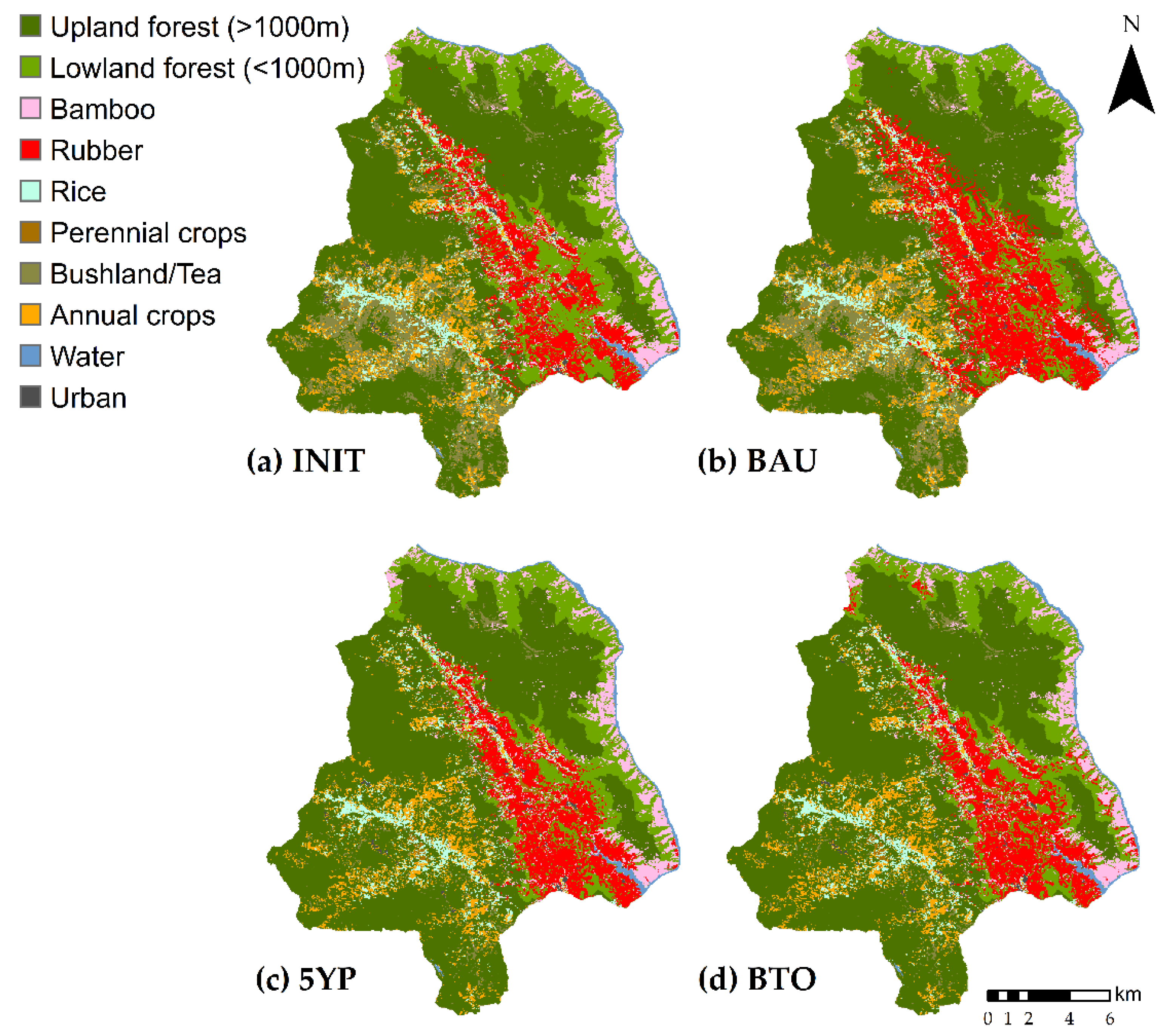
2.3. Land Use Change Scenarios

The implemented land use scenarios have been developed in the 5-year project SURUMER (Sustainable Rubber Cultivation in the Mekong Region) [62]. The aim of SURUMER was to develop stakeholder-validated land use and land management strategies to improve the sustainability of rubber production systems in Yunnan province. Stakeholders participating in the scenario development process included village heads and innovative farmers, prefecture administration, and local politicians [63,64]. Stakeholder workshops were held between January 2013 and October 2016 and were generally structured around presentations by SURUMER researchers, followed by interactive discussions. Scenario storylines were developed based on past land use changes and their perceived effects on the environment, local policy plans, and at a later stage, best practice recommendations based on preliminary results of field campaigns. Detailed information on the scenario development process can be found in Thellmann et al. [61] and Aenis & Wang [64]. Here, we focus on the implemented land use and land management rules leading to the land use maps we used as input for the modeling procedure with InVEST. The scenario outlines and maps were presented during the stakeholder workshops in order to confirm the viability of the introduced land use changes (e.g., spatial extent, property rights, land use restrictions) and the feasibility of management practices (e.g., weed management). The initial land use map of Nabanhe Reserve (2015) and the scenario maps resulting from the stakeholder participation process are depicted in Figure 2.
Land use as of 2015 was derived from Rapid Eye satellite imagery and serves as the initial condition for the InVEST models, as well as the baseline for three land use scenarios developed in the SURUMER project: (1) The Business-As-Usual (BAU) scenario features the unrestricted expansion of rubber plantations based on past expansion rates in the region [65,66]. This translates to an extension of 2% per year in relation to the area occupied by rubber in the previous year, which is targeted at lowland forest areas, and during the course of the scenario, upland forest areas. (2) The 5-Years-Plan (5YP) scenario is based on a local government plan [67]. It includes measures to reduce erosion and keep rubber plantations at suitable production locations only. These measures include the reforestation of bushland areas in the uplands and no further establishment of rubber plantations above 900 m.a.s.l. or on steep slopes (>23°). (3) The Balanced-Trade-Offs (BTO) scenario includes all measures featured in the 5YP scenario, but expands them based on the recommended land use and land management options developed by SURUMER. These recommendations include water protection zones around water sources and buffer strips along the two main streams (Mandian and Naban River) in Nabanhe Reserve. Both measures include the reforestation of degraded areas into secondary forest areas to trap sediments, nutrients, and pesticides in order to improve water quality. The land use scenarios have been set to end in 2040, as we think that any further land use change would be unreasonable to predict by a rule-based mechanism. Table 1 shows the percent coverage of land use categories for the initial condition of 2015 and the three land use scenarios.

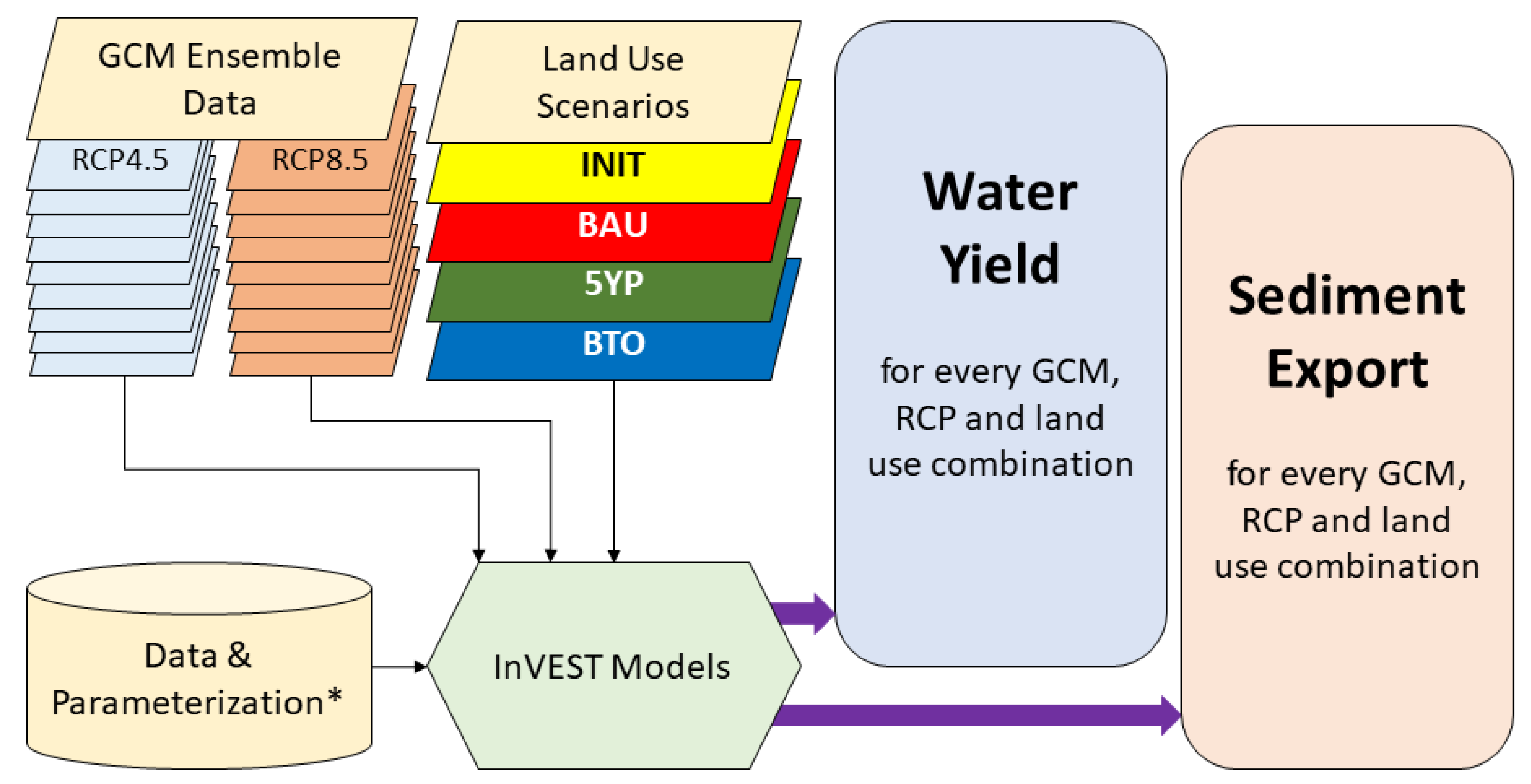
2.4. Modelling Framework

Erosion and water quantity were among the most relevant topics for the stakeholders in the SURUMER project [68]. We used InVEST (Version 3.3.3, The Natural Capital Project, Stanford University, Stanford, CA, USA, [12]) to model water yield and sediment export under the land use and climate change scenarios outlined in the previous sections. InVEST is a well-established modelling framework, which has been applied all around the globe [23,32,33,61,69,70,71]. The water yield model is based on the Budyko curve [72] and estimates annual water yield based on spatially explicit input data of annual average precipitation, annual potential evapotranspiration, root restricting layer depth, plant available water content, as well as rooting depths and evapotranspiration coefficients for each land use category. The sediment export model is based on the widely used USLE (Universal Soil Loss Equation) [73] and uses spatially explicit inputs such as a digital elevation model, annual rainfall erosivity, soil erodibility, as well as cover-management and support practice factors for every land use category. We refer to the InVEST user’s guide [12] for detailed descriptions of the biophysical relationships realized in the water yield and sediment export models. Details on model parameterization, application, and sensitivity analysis are given in Thellmann et al. [61]. Both the water yield and sediment export model were fitted to run-off and erosion field measurements in a sub-watershed in Nabanhe Reserve and then extrapolated to watershed scale [61,74].
Instead of using the stand-alone version of InVEST, we made use of InVEST in Python 2.7 in order to facilitate input data management and calculations using batch processing. Model outputs (TIFF-files) were exported to R Studio (Version 1.0.136, R Foundation for Statistical Computing, Vienna, Austria, [75]). We used the R library ‘raster’ to calculate spatial statistics. We applied two-tailed, paired Student’s t-tests in order to test if there are significant differences in the water yield, evapotranspiration, or sediment export results between (1) the land use scenarios, (2) the time slices of the climate scenarios, and (3) the two RCPs. We used ArcGIS (Version 10.3.1, Environmental Systems Research Institute, Redlands, CA, USA, [56]) and the R library ‘rasterVis’ to visualize spatially explicit results and OriginPro 2017 (Version b9.4.1.354, OriginLab Corporation, Northampton, MA, USA, [76]) to create plots of ensemble results. Scheme 1 provides a comprehensive overview of the modeling methodology.

3. Results

The following sections focus on InVEST results for water yield (3.1) and sediment export (3.2) averaged across all cells of the entire Nabanhe Reserve. Due to the large amount of data, spatial statistics and comparisons between the scenarios and baseline conditions are given in the Supplementary Materials (Figures S1–S18). Total water yield and total sediment export results in Nabanhe Reserve for every climate and land use scenario as well as percentage comparisons to baseline climate and land use conditions are listed in Table S1.

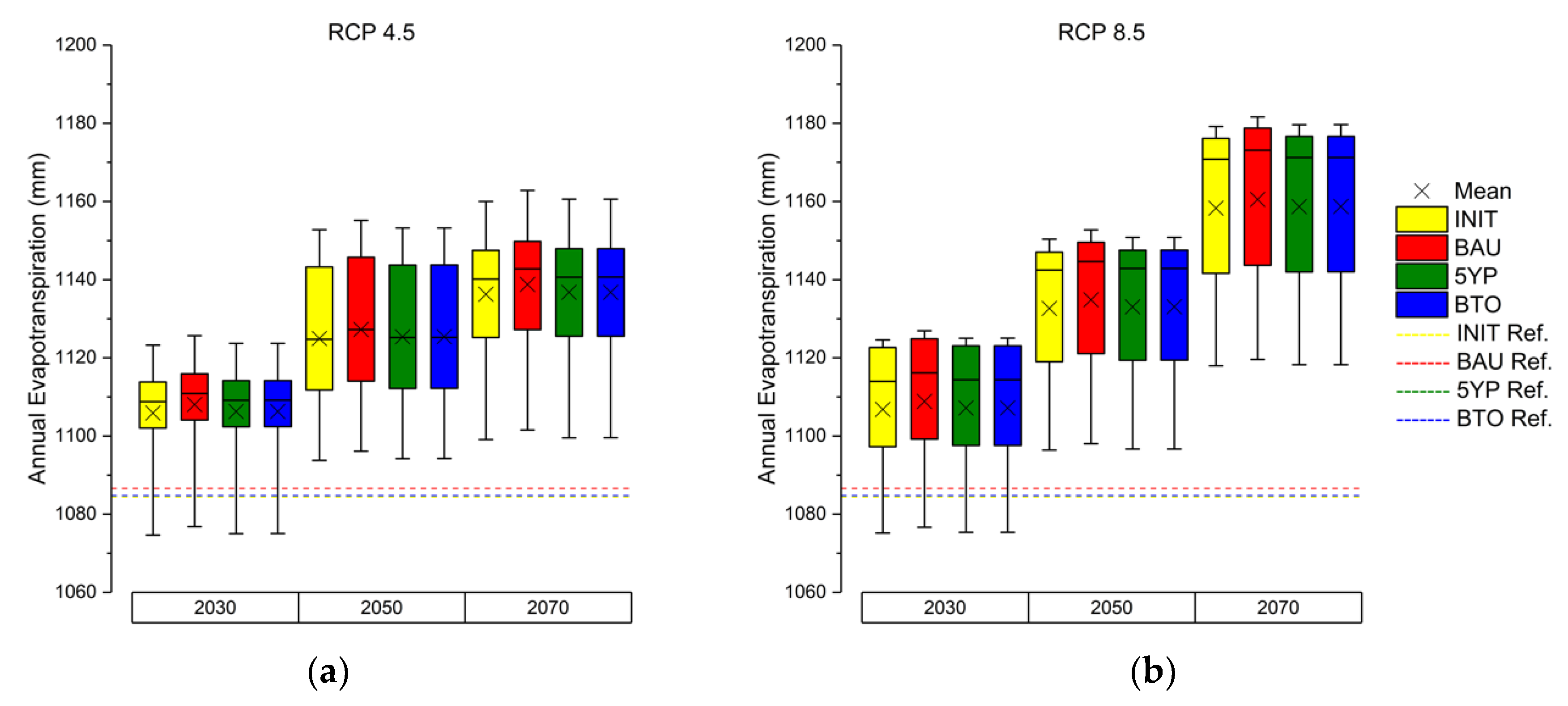
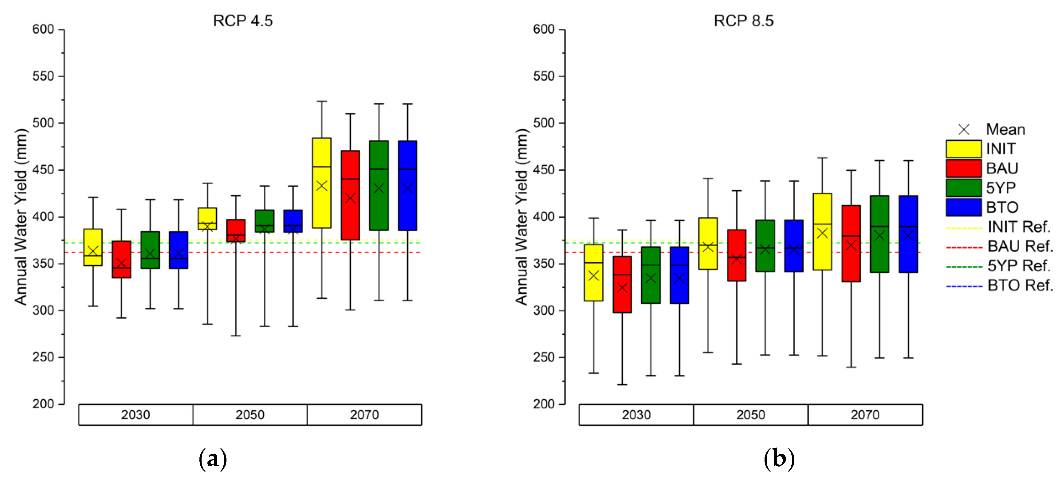
3.1. Evapotranspiration and Water Yield

In Figure 3, evapotranspiration simulation results are shown as an average across all cells in the study area to make comparisons between the scenarios easier. We observed an increasing trend in evapotranspiration during the course of both RCP scenarios, with higher evapotranspiration values in RCP 8.5. However, only the evapotranspiration results in 2070 were significantly different when comparing RCP 4.5 and RCP 8.5 (Table S4). Evapotranspiration in RCP 8.5 was skewed towards the higher values, with differences between median, 75 and 90 percentile ensemble values being in the range of tens of millimeters. For all time slices and RCP scenarios, evapotranspiration values for the BAU scenario were higher than in the other land use scenarios. Generally, the differences between the land use scenarios were minor in comparison to the large differences between the time slices (all with p < 0.5).
Water yield results were averaged across all cells in the study area in Figure 4. The simulated water yield for the baseline climate data and the initial land use was about 375 mm in Nabanhe Reserve. Differences between the initial land use and both 5YP and BTO were only ±1% at watershed scale for each climate condition (p < 0.5). On the other hand, the model results indicate a lower water yield ranging from −3.3% to −4.1% (depending on the climate condition) in BAU, when compared to the simulated water yield for the initial land use condition (p < 0.5). Both the median and the mean ensemble results of water yield for time slice 2030 in RCP 4.5 were lower in comparison to the baseline climate. This was due to increasing temperatures, which lead to higher potential evapotranspiration (Figure 3). As the mean and median precipitation values in the ensemble input data remained at the same level as the baseline climate data (Figure 1), the higher evapotranspiration leads to a reduction in simulated water yield in 2030 for both RCP 4.5 and RCP 8.5. An increasing trend for precipitation in 2050 and 2070 increased projected water yield also in RCP 4.5. Baseline evapotranspiration values (Figure 3) were in the same range as precipitation input (Figure 2). A two-tailed, paired Student’s t-test revealed no significant differences (p > 0.5) in water yield when comparing RCP 4.5 and RCP 8.5 (Table S2). Upland areas, which received the highest amount of precipitation and had lower potential evapotranspiration, contributed the largest share to the annual water yield in Nabanhe Reserve (Figure S1).

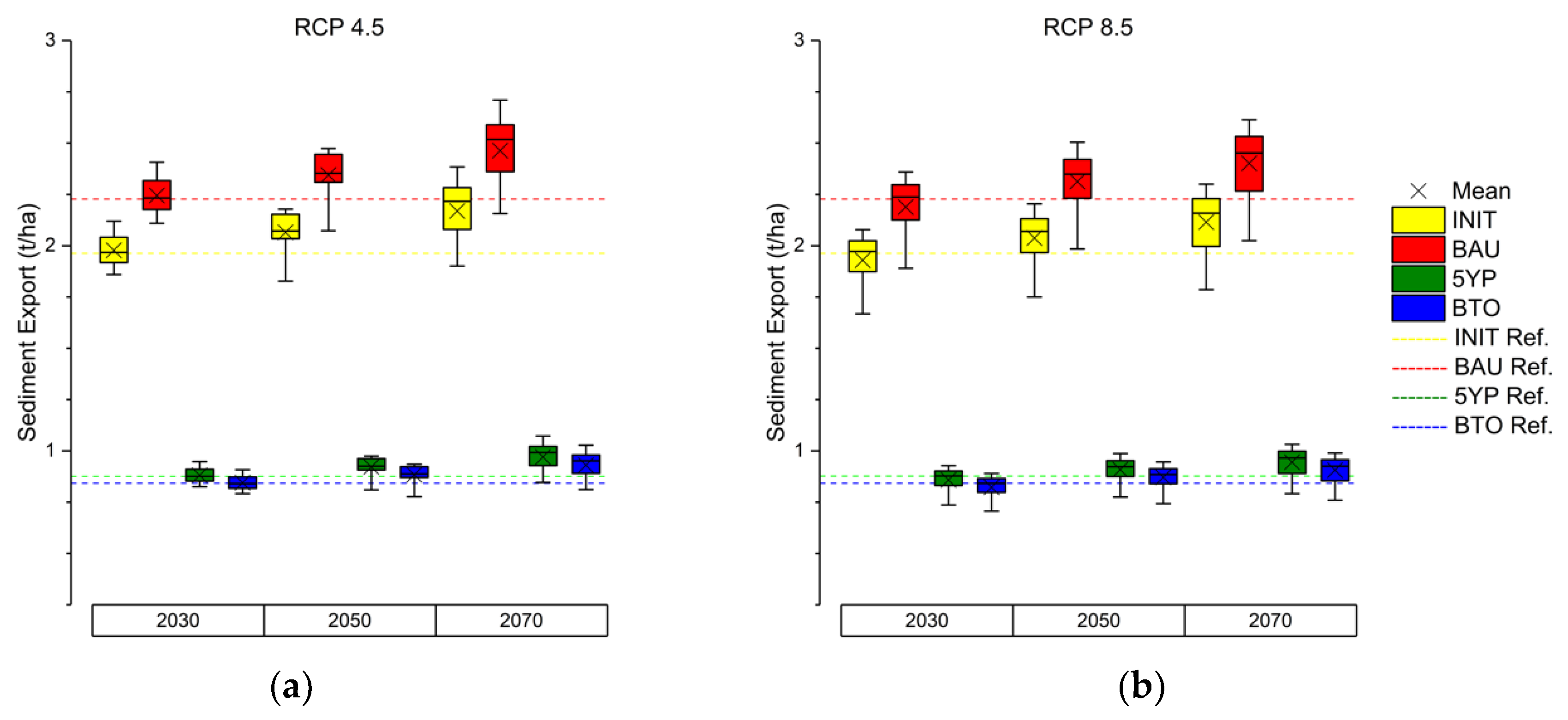
3.2. Sediment Export

Simulated sediment export for the baseline climate and land use was about 2 tons per hectare and year in Nabanhe Reserve. Sediment export averaged across all rubber plantation cells accounted for 1.38 t/ha for the initial land use and baseline climate (Figure S19). Land use categories with the highest amount of mean sediment export were annual agriculture (10.7 t/ha), bushland and tea plantations (8.5 t/ha), rice (3.6 t/ha), and perennial crops (3.2 t/ha) (Figure S19). In general, the simulation results indicate increases in sediment export from 2030 to 2070 for all land use scenarios in both RCPs (Figure 5). This is due to the increased amounts of precipitation in both RCP 4.5 and RCP 8.5. However, in RCP 4.5, only comparisons between 2030 and 2070 yield significantly different results (Table S6). For every land use scenario, sediment export results in RCP 4.5 were about 2.5% (2030), 0.9% (2050), and 1.6% (2070) higher in comparison to RCP 8.5. However, these differences were not statistically significant (p > 0.5) (Table S6). Unlike the results for water yield and evapotranspiration, the differences between the land use scenarios for sediment export were more pronounced as compared to the differences between the RCPs and time slices. In comparison to the initial condition of 2015, the model results indicate increased sediment export in BAU (up to 0.48 t/ha) and reductions for both 5YP and BTO (more than 1 t/ha) (p < 0.5). The results indicate that the reforestation measures and water protection zoning in the 5YP and BTO scenario slightly increased the sediment retention capacity of the landscape, as sediment from agricultural land use categories is more likely to be trapped by patches of natural vegetation in the down-slope sediment retention path in these scenarios (Figures S10 and S19). On the other hand, increased sediment export in BAU was mainly due to the expansion of rubber plantations at higher altitudes and steeper slopes (Figures S10 and S19).

4. Discussion

4.1. Climate Change Impacts

If one considers the climate change scenarios alone (using the initial land use data (INIT)), the model results indicate that both annual water yield and annual sediment export in Nabanhe Reserve are likely to increase with climate change by 2070 (p < 0.5). These results are in accordance with similar studies in Asia [33,77,78], which showed comparable increases in simulated water yield and sediment export under climate change scenarios. We expected to see significant differences between RCP 4.5 and RCP 8.5, however, with the exception of evapotranspiration results for the 2070 time slice, this was not the case. We conclude that the large difference in annual mean temperature in Nabanhe Reserve in the 2070 time slice (Figure 1a) is the main reason why only the evapotranspiration results for this time slice show a significant difference. Based on Figure 1b we conclude that the differences in annual precipitation between RCP 4.5 and RCP 8.5 are not large enough to lead to significant differences in both water yield and sediment export.
Our results for Nabanhe Reserve revealed higher percentage increases in water yield in the lowlands as a result of climate change as compared to more complex changes in the uplands (Figures S2–S9). Simulated water yield in the uplands was reduced (2030), relatively equal (2050), and slightly higher (2070) as compared to the baseline climate. This trend held true for both RCP 4.5 and RCP 8.5, albeit with smaller increases of water yield in the lowlands and larger decreases in the uplands for RCP 8.5. Hoyer & Chang [32] found that water yield estimates are especially sensitive to climate change in the lowlands, while sediment export is projected to increase under the higher erosivity from increased rainfall amounts. Bajracharya et al. [77] found that increases in temperature and precipitation show synergistic effects under climate change and increased water yield by over 50% at the outlet of the Kaligandaki basin of Nepal. We found the highest increase (~15%) in water yield in RCP 4.5 for the initial land use in Nabanhe Reserve. In Bajracharya et al. [77], glacier melt played an additional role in the local hydrology. As there are no glaciers in Nabanhe Reserve, effects of temperature increases throughout the next century will not be as severe as in other mountainous watersheds, e.g., the Kaligandaki basin in Nepal. In a watershed in southern Thailand, which is comparable in land use to Nabanhe Reserve, Trisurat et al. [33] showed that changes in rainfall (extreme value scenarios) exerted a stronger influence on water yield, but also on erosion and sediment export as compared to the effects of land use changes. However, the range of annual precipitation used as input for InVEST in Trisurat et al. [33] was also significantly larger (1980–3838 mm/year) than in this study.
Many studies on the impacts of climate change on water yield consider only changes in precipitation, but do not include changes in potential evapotranspiration (e.g., [32,33]). Our results also show significant increases in potential evapotranspiration as we approach the end of the century. As precipitation also increases, annual water yield in Nabanhe Reserve will be higher as compared to the baseline conditions at the end of the simulation. However, in both RCP 4.5 and RCP 8.5, the increases in temperature and evapotranspiration lead to a reduction of water yield in 2030. This reduction was most severe in RCP 8.5, with a reduction of annual water yield of more than 10% for every land use scenario. We can extrapolate that particularly dry years may have a more pronounced effect on the water balance in the future as the higher potential evapotranspiration increases the probability for periods of water scarcity, especially in the dry seasons.

4.2. Land Use Change and Management Implications

The land use scenarios we have analyzed are based on an intensive stakeholder dialogue and represent a transdisciplinary work effort by rubber farmers, policy-makers and scientists alike. During the workshops, stakeholders expressed that the current situation of rubber cultivation is difficult to change for the following reasons: (1) In comparison to other cash crops, there is still a relatively high price to be gained for rubber; (2) No more land is available for the cultivation of other crops; (3) Farmers have invested in their plantations and are hesitant to replace them before the end of the economic life cycle; (4) Farmers know how to manage rubber plantations and lack experience with other crops; (5) Farmers want to continue growing rubber, even under less than optimal market and environmental conditions [74].
Most of the areas in Nabanhe Reserve featuring optimal growth conditions for rubber were already occupied with rubber plantations at the initial year of the simulations (2015). Therefore, the extension of rubber plantations (from 9.2% to 15.2% of Nabanhe Reserve) in the BAU scenario is mostly targeted at locations above 900 m.a.s.l., of which a large part is also characterized by steep slopes (>23°). For the BAU scenario, our results revealed the highest water yield reductions and also the highest sediment export for all simulated climate conditions. Rubber expansions on high altitudes and steep slopes should, therefore, be prevented. During the workshops, stakeholders critically commented further rubber expansions as they saw them as rather unlikely, due to the aforementioned reasons [74]. Nevertheless, the trend of rubber expansions into higher altitudes and steep slopes has been observed all over Xishuangbanna [22]. As in other watersheds [79,80], upland areas have the highest water regulation capacity. Therefore, these should be targeted for protection [80]. Reforesting and protecting these areas were the main aims of both the 5YP and BTO scenario. The BTO scenario featured the highest sediment retention capacity with the implementation of riverine buffer strips, water protection zones and reduced herbicide application in rubber plantations. However, in comparison to the 5YP scenario, the additional benefits of these measures were very small (roughly 0.03 t/ha), as upland reforestation alone significantly reduced exported sediments (roughly 1 t/ha).
Further research should be aimed at cost-benefit analysis and at assessing the effect of these measures on water quality (e.g., fertilizer and pesticide residues). Additional benefits of the BTO scenario in comparison to the 5YP such as improved habitat quality and rubber yields have been shown in other studies [61,81], albeit without the integration of climate change impacts. The land management measures of the BTO scenario have been met with higher approval rates by the stakeholders in comparison to the other two scenarios [74]. Water protection was expressed to be of utmost importance by the stakeholders, as they already experienced the reduction of available drinking water resources [74].
Rubber cultivation provides on average over 40% of smallholder incomes in Xishuangbanna, so household incomes are at risk due to reduced diversification and the dependence on market prices [82]. The reforestation measures as described in BTO (and 5YP to a lesser degree) are unlikely to be adopted by farmers without any economic incentives. Although stakeholders were generally positive about the assumptions in both 5YP and BTO, they were also doubtful about their implementation [74]. Suggestions to completely dispense with weed control measures have been met with disapproval by the farmers, as it reduces tree accessibility for tapping and increases the probability to encounter poisonous caterpillars [83]. Intercropping (with e.g., maize or tea), as a measure to reduce erosion, was discussed controversially during the stakeholder workshops [74]. So far, intercropping methods for rubber plantations have only shown low adoption rates by local farmers, even though these methods are encouraged by the government and have the potential to improve sediment retention and diversify household income sources [84].

4.3. Uncertainties and Limitations of the Study

InVEST has been developed as a policy support tool to enable researchers and practitioners to assess the impact of land use planning decisions on ESS. Compared to other, more specialized hydrological models (e.g., SWAT), InVEST represents bio-physical processes in a simplified manner. The choice of this model may not seem ideal for assessing the impact of climate change on hydrological ESS. However, more sophisticated models are much more demanding with regard to the temporal resolution of input data (e.g., daily resolution for SWAT), which makes them less compatible with freely available GCM data. As InVEST was designed to work with long-term average input data, we argue that it is a suitable choice for comparing the impacts of long-term changes in climatic variables on ESS.
Many hydrological ESS modelling studies rely on one or few precipitation and temperature datasets as input, particularly in tropical regions where hydro-meteorological data are often scarce. This makes conclusions about the absolute amount of available water highly dependent on the selected input data [85]. In cases of data scarcity, van Soesbergen & Mulligan [85] suggest percentage comparisons to baseline conditions as an alternative to assess future adaptation options. Shrestha et al. [29] emphasized the need for multi-climate model evaluations of future hydrological conditions for climate change adaptation and sediment management. We included an ensemble of climate datasets derived from nine GCMs in order to define an uncertainty envelope for the hydrological ESS model results (Figure 3, Figure 4 and Figure 5) and provided percentage comparisons to baseline conditions (Table S1). For the selection of climate data, McSweeney et al. [44] recommended to retain a subset of 8–10 GCMs in order to ensure plausible dispersion while avoiding the least realistic model predictions for a particular study region. As expected, large uncertainties exist in all of the hydrological variables due to the differences in the climate model projections. The spread in the results of water yield (and precipitation input) is generally larger at higher altitudes in Nabanhe Reserve. These areas are also the source of the largest quantities of run-off (Figures S1–S9). These results are not particular for Nabanhe Reserve, but have also been assessed in other basins spanning steep gradients in elevation [86,87]. Uncertainties in the results for sediment export are highest in the down-slope sediment retention pathways (Figures S11–S18). Uncertainties stem from the different assumptions and parameterizations of the GCMs, but also from downscaling temperature and precipitation datasets to a finer resolution.
As the InVEST water yield model works on an annual basis, it is not able to capture intra-annual variability of temperature, precipitation, and evapotranspiration patterns. This is most likely the greatest limitation of our approach, as annual evapotranspiration from rubber trees has been linked with high late dry season water use from rapid refoliation after leaf flush as well as very high wet season evapotranspiration [88]. The same limitation also applies to the sediment export model, as the timing and the amount of daily precipitation intensity also have a large influence on potential erosion [78]. Furthermore, the InVEST water yield model is limited in its representation of plant physiology. An increased intra-annual resolution would open up the possibility to include more phenological variables (e.g., vapor pressure deficit, leaf area or photoperiod) in order to improve how the transpiration of plants is represented in the water yield model. Combined with the available monthly GCM data, this would allow for predictions of water availability in regard to seasonal highs and lows, which in turn would be more beneficial for watershed management than our current approach. Similar benefits would apply to weed management in rubber plantations, as the timing and frequency of herbicide application in rubber plantations has been shown to be highly influential in rubber plantations [83]. Future modelling efforts including improved plant physiology, intra-annual or seasonal variability and extreme wet/dry climate conditions are needed to shed more light on temporal patterns of water provisioning and sedimentation in Nabanhe Reserve.

5. Conclusions

Should the expansion of rubber plantations in Nabanhe Reserve continue, the increases in sediment export will be amplified further under the wetter and warmer climate. In addition, we conclude that the effects of land use and land management decisions on water yield in Nabanhe Reserve are relatively minor when compared to the effects that future climate change will exert on water yield. Our results can contribute to an effective management of erosion and sedimentation in Nabanhe Reserve and provide useful insights for future water availability and sediment export under the effects of climate change in the watershed. The method we applied can easily be transferred to other regions facing comparable land use situations, as InVEST and the IPCC5 data are freely available. Furthermore, up-scaling our methodology to larger areas could be beneficial for hydro-power planning in the area [89,90], as it includes information about annual water and sediment volumes under the effect of climate change.

Supplementary Materials

The following are available online at https://www.mdpi.com/1999-4907/10/2/176/s1, Figure S1: Water yield results for every land use scenario and the baseline climate data. INIT: Initial land use in 2015, BAU: Business-As-Usual, 5YP: 5-Years-Plan, BTO: Balanced-Trade-Offs, Figure S2: Water yield and standard deviation results in Nabanhe Reserve for the initial land use in 2015 (INIT) under RCP 4.5 climate data, Figure S3: Water yield and standard deviation results in Nabanhe Reserve for the initial land use in 2015 (INIT) under RCP 8.5 climate data, Figure S4: Water yield and standard deviation results in Nabanhe Reserve for the Business-As-Usual scenario (BAU) under RCP 4.5 climate data, Figure S5: Water yield and standard deviation results in Nabanhe Reserve for the Business-As-Usual scenario (BAU) under RCP 8.5 climate data, Figure S6: Water yield and standard deviation results in Nabanhe Reserve for the 5-Years-Plan scenario (5YP) under RCP 4.5 climate data, Figure S7: Water yield and standard deviation results in Nabanhe Reserve for the 5-Years-Plan scenario (5YP) under RCP 8.5 climate data, Figure S8: Water yield and standard deviation results in Nabanhe Reserve for the Balanced-Trade-Offs scenario (BTO) under RCP 4.5 climate data, Figure S9: Water yield and standard deviation results in Nabanhe Reserve for the Balanced-Trade-Offs scenario (BTO) under RCP 8.5 climate data, Figure S10: Sediment export results for every land use scenario and the baseline climate data. INIT: Initial land use in 2015, BAU: Business-As-Usual, 5YP: 5-Years-Plan, BTO: Balanced-Trade-Offs, Figure S11: Sediment export and standard deviation results in Nabanhe Reserve for the initial land use (INIT) under RCP 4.5 climate data, Figure S12: Sediment export and standard deviation results in Nabanhe Reserve for the initial land use (INIT) under RCP 8.5 climate data, Figure S13: Sediment export and standard deviation results in Nabanhe Reserve for the Business-As-Usual scenario (BAU) under RCP 4.5 climate data, Figure S14: Sediment export and standard deviation results in Nabanhe Reserve for the Business-As-Usual scenario (BAU) under RCP 8.5 climate data, Figure S15: Sediment export and standard deviation results in Nabanhe Reserve for the 5-Years-Plan scenario (5YP) under RCP 4.5 climate data, Figure S16: Sediment export and standard deviation results in Nabanhe Reserve for the 5-Years-Plan scenario (5YP) under RCP 8.5 climate data, Figure S17: Sediment export and standard deviation results in Nabanhe Reserve for the Balanced-Trade-Offs scenario (BTO) under RCP 4.5 climate data, Figure S18: Sediment export and standard deviation results in Nabanhe Reserve for the Balanced-Trade-Offs scenario (BTO) under RCP 8.5 climate data, Figure S19: Sediment export averaged over every land use category in Nabanhe Reserve for the initial land use (INIT) and baseline climate. We calculated these values by summing the sediment export amounts from each land use category and divided them by the areal extent of the respective land use category in Nabanhe Reserve, Table S1: Total water yield and total sediment export in Nabanhe Reserve estimated by InVEST for all climate and land use scenarios as well as percentage comparisons to the baseline climate and land use conditions. Table S2: Simulation results of the InVEST water yield model for the land use scenarios and each General Circulation Model (GCM) in Nabanhe Reserve, Table S3: Results of a two-tailed, paired Student’s t-test to determine significant differences between water yield model results. Green values indicate significant differences (p < 0.05), red values indicate no significant difference (p > 0.05), Table S4: Simulation results for evapotranspiration for the land use scenarios and each GCM in Nabanhe Reserve, Table S5: Results of a two-tailed, paired Student’s t-test to determine significant differences between evapotranspiration model results. Green values indicate significant differences (p < 0.05), red values indicate no significant difference (p > 0.05), Table S6: Simulation results for sediment export for the land use scenarios and each GCM in Nabanhe Reserve, Table S7: Results of a two-tailed, paired Student’s t-test to determine significant differences between sediment export model results. Green values indicate significant differences (p < 0.05), red values indicate no significant difference (p > 0.05).

Author Contributions

Conceptualization, K.T. and M.C.; methodology, K.T., R.G. and M.C.; software, K.T.; validation, K.T.; formal analysis, K.T.; investigation, K.T.; resources, G.C. and F.A.; data curation, K.T. and R.G.; writing-original draft preparation, K.T.; writing-review and editing, K.T., M.C., G.C. and F.A.; visualization, K.T.; supervision, M.C., G.C. and F.A.; project administration, M.C., G.C. and F.A.; funding acquisition, K.T., M.C., G.C. and F.A.

Funding

This research was funded by the German Federal Ministry of Education and Research (BMBF), grant number FKZ 01LL0919, FKZ 16PGF0105 and by Deutsche Forschungsgemeinschaft CO 1864/2-1. We greatly acknowledge the financial support of the “Water-People-Agriculture” Research Training Group funded by the Anton & Petra-Ehrmann-Stiftung.

Acknowledgments

Thank you to the SURUMER team for their support and collaboration. We would also like to thank the two anonymous reviewers for their comments and suggestions, which strengthened the quality of the paper substantially.

Conflicts of Interest

The authors declare no conflict of interest.

References

  1. Reid, W.V.; Mooney, H.A.; Cropper, A.; Capistrano, D.; Carpenter, S.R.; Chopra, K.; Dasgupta, P.; Dietz, T.; Duraiappah, A.K.; Hassan, R.; et al. Millenium Ecosystem Assessment. In Ecosystems and Human Well-being: Synthesis; Island Press: Washington, DC, USA, 2005. [Google Scholar]
  2. Newbold, T.; Hudson, L.N.; Hill, S.L.L.; Contu, S.; Lysenko, I.; Senior, R.A.; Börger, L.; Bennett, D.J.; Choimes, A.; Collen, B.; et al. Global effects of land use on local terrestrial biodiversity. Nature 2015, 520, 45–50. [Google Scholar] [CrossRef] [PubMed] [Green Version]
  3. Foley, J.A.; DeFries, R.; Asner, G.P.; Barford, C.; Bonan, G.; Carpenter, S.R.; Chapin, F.S.; Coe, M.T.; Daily, G.C.; Gibbs, H.K.; et al. Global consequences of land use. Science 2005, 309, 570–574. [Google Scholar] [CrossRef] [PubMed]
  4. Grimm, N.B.; Groffman, P.; Staudinger, M.; Tallis, H. Climate change impacts on ecosystems and ecosystem services in the United States: Process and prospects for sustained assessment. Clim. Chang. 2016, 135, 97–109. [Google Scholar] [CrossRef]
  5. Metzger, M.J.; Rounsevell, M.D.A.; Acosta-Michlik, L.; Leemans, R.; Schröter, D. The vulnerability of ecosystem services to land use change. Agric. Ecosyst. Environ. 2006, 114, 69–85. [Google Scholar] [CrossRef]
  6. Daily, G.C.; Matson, P.A. Ecosystem services: From theory to implementation. Proc. Natl. Acad. Sci. USA 2008, 105, 9455–9456. [Google Scholar] [CrossRef] [PubMed]
  7. Fisher, B.; Christie, M.; Aronson, J.; Braat, L.; Gowdy, J.; Haines-Young, R.; Maltby, E.; Neuville, A.; Polasky, S.; Portela, R.; et al. TEEB. The Economics of Ecosystems and Biodiversity: Ecological and Economic Foundations; Kumar, P., Ed.; Routledge: London, UK, 2012; ISBN 978-0-415-50108-8. [Google Scholar]
  8. Perrings, C.; Duraiappah, A.; Larigauderie, A.; Mooney, H. The Biodiversity and Ecosystem Services Science-Policy Interface. Science 2011, 331, 1139–1140. [Google Scholar] [CrossRef] [PubMed]
  9. Scholes, R.J.; Montanarella, L.; Brainich, A.; Barger, N.; ten Brink, B.; Cantele, M.; Erasmus, B.; Fisher, J.; Gardner, T.; Holland, T.G.; et al. IPBES Summary for Policymakers of the Assessment Report on Land Degradation and Restoration of the Intergovernmental Science-Policy Platform on Biodiversity and Ecosystem Services; IPBES Secretariat: Bonn, Germany, 2018; ISBN 978-3-947851-04-1. [Google Scholar]
  10. Martínez-Harms, M.J.; Balvanera, P. Methods for mapping ecosystem service supply: A review. Int. J. Biodivers. Sci. Ecosyst. Serv. Manag. 2012, 8, 17–25. [Google Scholar] [CrossRef]
  11. SWAT Soil & Water Assessment Tool. Available online: https://swat.tamu.edu/ (accessed on 7 November 2018).
  12. Sharp, R.; Tallis, H.; Ricketts, T.; Guerry, A.D.; Wood, S.A.; Chaplin-Kramer, R.; Nelson, E.; Ennaanay, D.; Wolny, S.; Olwero, N.; et al. InVEST 3.3.3 User’s Guide. The Natural Capital Project: Stanford University, University of Minnesota, The Nature Conservancy, and World Wildlife Fund. 2016. Available online: http://data.naturalcapitalproject.org/nightly-build/invest-users-guide/html/ (accessed on 7 November 2018).
  13. Ochoa, V.; Urbina-Cardona, N. Tools for spatially modeling ecosystem services: Publication trends, conceptual reflections and future challenges. Ecosyst. Serv. 2017, 26, 155–169. [Google Scholar] [CrossRef]
  14. Kharin, V.V.; Zwiers, F.W.; Zhang, X.; Wehner, M. Changes in temperature and precipitation extremes in the CMIP5 ensemble. Clim. Chang. 2013, 119, 345–357. [Google Scholar] [CrossRef]
  15. Alexander, L.V.; Zhang, X.; Peterson, T.C.; Caesar, J.; Gleason, B.; Klein Tank, A.M.G.; Haylock, M.; Collins, D.; Trewin, B.; Rahimzadeh, F.; et al. Global observed changes in daily climate extremes of temperature and precipitation. J. Geophys. Res. 2006, 111. [Google Scholar] [CrossRef] [Green Version]
  16. Trenberth, K.E.; Dai, A.; Rasmussen, R.M.; Parsons, D.B. The Changing Character of Precipitation. Bull. Am. Meteorol. Soc. 2003, 84, 1205–1218. [Google Scholar] [CrossRef] [Green Version]
  17. Alexander, L.V.; Allen, S.K.; Bindoff, N.L.; Bréon, F.-M.; Church, J.A.; Cubasch, U.; Emori, S.; Forster, P.; Friedlingstein, P.; Gillett, N.; et al. IPCC Summary for Policymakers. In Climate Change 2013: The Physical Science Basis. Contribution of Working Group I to the Fifth Assessment Report of the Intergovernmental Panel on Climate Change; Cambridge University Press: Cambridge, UK; New York, NY, USA, 2013. [Google Scholar]
  18. Ziegler, A.D.; Bruun, T.B.; Guardiola-Claramonte, M.; Giambelluca, T.W.; Lawrence, D.; Thanh Lam, N. Environmental consequences of the demise in swidden cultivation in montane mainland southeast asia: Hydrology and geomorphology. Hum. Ecol. 2009, 37, 361–373. [Google Scholar] [CrossRef]
  19. Dressler, W.H.; Wilson, D.; Clendenning, J.; Cramb, R.; Keenan, R.; Mahanty, S.; Bruun, T.B.; Mertz, O.; Lasco, R.D. The impact of swidden decline on livelihoods and ecosystem services in Southeast Asia: A review of the evidence from 1990 to 2015. Ambio 2017, 46, 291–310. [Google Scholar] [CrossRef] [PubMed]
  20. Li, H.; Aide, T.M.; Ma, Y.; Liu, W.; Cao, M. Demand for rubber is causing the loss of high diversity rain forest in SW China. Biodivers. Conserv. 2007, 16, 1731–1745. [Google Scholar] [CrossRef]
  21. Smajgl, A.; Xu, J.; Egan, S.; Yi, Z.-F.; Ward, J.; Su, Y. Assessing the effectiveness of payments for ecosystem services for diversifying rubber in Yunnan, China. Environ. Model. Softw. 2015, 69, 187–195. [Google Scholar] [CrossRef]
  22. Chen, H.; Yi, Z.-F.; Schmidt-Vogt, D.; Ahrends, A.; Beckschäfer, P.; Kleinn, C.; Ranjitkar, S.; Xu, J. Pushing the limits: The pattern and dynamics of rubber monoculture expansion in Xishuangbanna, SW China. PLoS ONE 2016, 11, 1–15. [Google Scholar] [CrossRef] [PubMed]
  23. Thellmann, K.; Cotter, M.; Baumgartner, S.; Treydte, A.; Cadisch, G.; Asch, F. Tipping Points in the Supply of Ecosystem Services of a Mountainous Watershed in Southeast Asia. Sustainability 2018, 10, 2418. [Google Scholar] [CrossRef]
  24. Arunyawat, S.; Shrestha, R. Assessing Land Use Change and Its Impact on Ecosystem Services in Northern Thailand. Sustainability 2016, 8, 768. [Google Scholar] [CrossRef]
  25. Wu, Z.-L.; Liu, H.-M.; Liu, L.-Y. Rubber cultivation and sustainable development in Xishuangbanna, China. Int. J. Sustain. Dev. World Ecol. 2001, 8, 337–345. [Google Scholar] [CrossRef]
  26. Liu, H.; Blagodatsky, S.; Giese, M.; Liu, F.; Xu, J.; Cadisch, G. Impact of herbicide application on soil erosion and induced carbon loss in a rubber plantation of Southwest China. Catena 2016, 145, 180–192. [Google Scholar] [CrossRef]
  27. Guardiola-Claramonte, M.; Troch, P.A.; Ziegler, A.D.; Giambelluca, T.W.; Durcik, M.; Vogler, J.B.; Nullet, M.A. Hydrologic effects of the expansion of rubber (Hevea brasiliensis) in a tropical catchment. Ecohydrology 2010, 3, 306–314. [Google Scholar] [CrossRef]
  28. Eastham, J.; Mpelasoka, M.; Mainuddin, C.; Ticehurst, C.; Dyce, P.; Hodgson, G.; Ali, R.; Kirby, M. Mekong River Basin water resources assessment: Impacts of climate change. CSIRO Water Healthy Ctry. Natl. Res. Flagship 2008, 153. [Google Scholar]
  29. Shrestha, B.; Babel, M.S.; Maskey, S.; van Griensven, A.; Uhlenbrook, S.; Green, A.; Akkharath, I. Impact of climate change on sediment yield in the Mekong River basin: A case study of the Nam Ou basin, Lao PDR. Hydrol. Earth Syst. Sci. 2013, 17, 1–20. [Google Scholar] [CrossRef]
  30. Zhu, Y.-M.; Lu, X.X.; Zhou, Y. Sediment flux sensitivity to climate change: A case study in the Longchuanjiang catchment of the upper Yangtze River, China. Glob. Planet. Chang. 2008, 60, 429–442. [Google Scholar] [CrossRef]
  31. Phan, D.B.; Wu, C.C.; Hsieh, S.C. Impact of climate change on stream discharge and sediment yield in Northern Viet Nam. Water Resour. 2011, 38, 827–836. [Google Scholar] [CrossRef]
  32. Hoyer, R.; Chang, H. Assessment of freshwater ecosystem services in the tualatin and Yamhill basins under climate change and urbanization. Appl. Geogr. 2014, 53, 402–416. [Google Scholar] [CrossRef]
  33. Trisurat, Y.; Eawpanich, P.; Kalliola, R. Integrating land use and climate change scenarios and models into assessment of forested watershed services in Southern Thailand. Environ. Res. 2016, 147, 611–620. [Google Scholar] [CrossRef]
  34. Li, Z.; Zhang, Y.; Wang, S.; Yuan, G.; Yang, Y.; Cao, M. Evapotranspiration of a tropical rain forest in Xishuangbanna, Southwest China. Hydrol. Process. 2010, 24, 2405–2416. [Google Scholar] [CrossRef]
  35. Myers, N.; Mittermeier, R.A.; Mittermeier, C.G.; Da Fonseca, G.A.B.; Kent, J. Biodiversity hotspots for conservation priorities. Nature 2000, 403, 853–858. [Google Scholar] [CrossRef]
  36. Zhang, J.; Cao, M. Tropical forest vegetation of Xishuangbanna, SW China and its secondary changes, with special reference to some problems in local nature conservation. Biol. Conserv. 1995, 73, 229–238. [Google Scholar] [CrossRef]
  37. UNESCO Biosphere Reserves | United Nations Educational, Scientific and Cultural Organization. Available online: http://www.unesco.org/new/en/natural-sciences/environment/ecological-sciences/biosphere-reserves/ (accessed on 1 February 2019).
  38. Li, H.; Ma, Y.; Aide, T.M.; Liu, W. Past, present and future land-use in Xishuangbanna, China and the implications for carbon dynamics. For. Ecol. Manag. 2008, 255, 16–24. [Google Scholar] [CrossRef]
  39. Hijmans, R.J.; Cameron, S.E.; Parra, J.L.; Jones, P.G.; Jarvis, A. Very high resolution interpolated climate surfaces for global land areas. Int. J. Climatol. 2005, 25, 1965–1978. [Google Scholar] [CrossRef] [Green Version]
  40. World Clim-Global Climate Data | Free Climate Data for Ecological Modeling and GIS. Available online: http://www.worldclim.org/ (accessed on 20 October 2017).
  41. Thomson, A.M.; Calvin, K.V.; Smith, S.J.; Kyle, G.P.; Volke, A.; Patel, P.; Delgado-Arias, S.; Bond-Lamberty, B.; Wise, M.A.; Clarke, L.E.; et al. RCP4.5: A pathway for stabilization of radiative forcing by 2100. Clim. Chang. 2011, 109, 77–94. [Google Scholar] [CrossRef]
  42. Riahi, K.; Rao, S.; Krey, V.; Cho, C.; Chirkov, V.; Fischer, G.; Kindermann, G.; Nakicenovic, N.; Rafaj, P. RCP 8.5—A scenario of comparatively high greenhouse gas emissions. Clim. Chang. 2011, 109, 33–57. [Google Scholar] [CrossRef] [Green Version]
  43. Golbon, R.; Cotter, M.; Sauerborn, J. Climate change impact assessment on the potential rubber cultivating area in the Greater Mekong Subregion. Environ. Res. Lett. 2018, 13, 084002. [Google Scholar] [CrossRef]
  44. McSweeney, C.F.; Jones, R.G.; Lee, R.W.; Rowell, D.P. Selecting CMIP5 GCMs for downscaling over multiple regions. Clim. Dyn. 2015, 44, 3237–3260. [Google Scholar] [CrossRef]
  45. Bi, D.; Dix, M.; Marsland, S.; O’Farrell, S.; Rashid, H.; Uotila, P.; Hirst, A.; Kowalczyk, E.; Golebiewski, M.; Sullivan, A.; et al. The ACCESS coupled model: Description, control climate and evaluation. Aust. Meteorol. Oceanogr. J. 2013, 63, 41–64. [Google Scholar] [CrossRef]
  46. Dix, M.; Vohralik, P.; Bi, D.; Rashid, H.; Marsland, S.; O’Farrell, S.; Uotila, P.; Hirst, T.; Kowalczyk, E.; Sullivan, A.; et al. The ACCESS coupled model: Documentation of core CMIP5 simulations and initial results. Aust. Meteorol. Oceanogr. J. 2013, 63, 83–99. [Google Scholar] [CrossRef]
  47. Xin, X.; Zhang, L.; Zhang, J.; Wu, T.; Fang, Y. Climate Change Projections over East Asia with BCC_CSM1.1 Climate Model under RCP Scenarios. J. Meteorol. Soc. Jpn. Ser II 2013, 91, 413–429. [Google Scholar] [CrossRef] [Green Version]
  48. Gent, P.R.; Danabasoglu, G.; Donner, L.J.; Holland, M.M.; Hunke, E.C.; Jayne, S.R.; Lawrence, D.M.; Neale, R.B.; Rasch, P.J.; Vertenstein, M.; et al. The Community Climate System Model Version 4. J. Clim. 2011, 24, 4973–4991. [Google Scholar] [CrossRef] [Green Version]
  49. Donner, L.J.; Wyman, B.L.; Hemler, R.S.; Horowitz, L.W.; Ming, Y.; Zhao, M.; Golaz, J.-C.; Ginoux, P.; Lin, S.-J.; Schwarzkopf, M.D.; et al. The Dynamical Core, Physical Parameterizations, and Basic Simulation Characteristics of the Atmospheric Component AM3 of the GFDL Global Coupled Model CM3. J. Clim. 2011, 24, 3484–3519. [Google Scholar] [CrossRef]
  50. Martin, G.M.; Bellouin, N.; Collins, W.J.; Culverwell, I.D.; Halloran, P.R.; Hardiman, S.C.; Hinton, T.J.; Jones, C.D.; McDonald, R.E.; McLaren, A.J.; et al. The HadGEM2 family of Met Office Unified Model climate configurations. Geosci. Model. Dev. 2011, 4, 723–757. [Google Scholar] [Green Version]
  51. Dufresne, J.-L.; Foujols, M.-A.; Denvil, S.; Caubel, A.; Marti, O.; Aumont, O.; Balkanski, Y.; Bekki, S.; Bellenger, H.; Benshila, R.; et al. Climate change projections using the IPSL-CM5 Earth System Model: From CMIP3 to CMIP5. Clim. Dyn. 2013, 40, 2123–2165. [Google Scholar] [CrossRef]
  52. Yukimoto, S.; Adachi, Y.; Hosaka, M.; Sakami, T.; Yoshimura, H.; Hirabara, M.; Tanaka, T.Y.; Shindo, E.; Tsujino, H.; Deushi, M.; et al. A New Global Climate Model of the Meteorological Research Institute: MRI-CGCM3: Model Description and Basic Performance. J. Meteorol. Soc. Jpn. 2012, 90, 23–64. [Google Scholar] [CrossRef]
  53. Giorgetta, M.A.; Jungclaus, J.; Reick, C.H.; Legutke, S.; Bader, J.; Böttinger, M.; Brovkin, V.; Crueger, T.; Esch, M.; Fieg, K.; et al. Climate and carbon cycle changes from 1850 to 2100 in MPI-ESM simulations for the Coupled Model Intercomparison Project phase 5: Climate Changes in MPI-ESM. J. Adv. Model. Earth Syst. 2013, 5, 572–597. [Google Scholar] [CrossRef]
  54. Bentsen, M.; Bethke, I.; Debernard, J.B.; Iversen, T.; Kirkevåg, A.; Seland, O.; Drange, H.; Roelandt, C.; Seierstad, I.A.; Hoose, C.; et al. The Norwegian Earth System Model, NorESM1-M—Part 1: Description and basic evaluation of the physical climate. Geosci. Model. Dev. 2013, 6, 687–720. [Google Scholar] [CrossRef]
  55. Data-CCAFS Climate. Available online: http://www.ccafs-climate.org/data_spatial_downscaling/ (accessed on 6 November 2018).
  56. ESRI ArcGIS 10.3.1.; Environmental Systems Research Institute: Redlands, CA, USA, 2015.
  57. Global Aridity and PET Database/CGIAR-CSI. Available online: http://www.cgiar-csi.org/data/global-aridity-and-pet-database (accessed on 20 October 2017).
  58. Zomer, R.J.; Bossio, D.A.; Trabucco, A.; Yuanjie, L.; Gupta, D.C.; Singh, V.P. Trees and Water: Smallholder Agroforestry on Irrigated Lands in Northern India; International Water Management Institute: Colombo, Sri Lanka, 2007; p. 47. [Google Scholar]
  59. Zomer, R.J.; Trabucco, A.; Bossio, D.A.; Verchot, L.V. Climate change mitigation: A spatial analysis of global land suitability for clean development mechanism afforestation and reforestation. Agric. Ecosyst. Environ. 2008, 126, 67–80. [Google Scholar] [CrossRef]
  60. Hargreaves, G.H.; Allen, R.G. History and Evaluation of Hargreaves Evapotranspiration Equation. J. Irrig. Drain. Eng. 2003, 129, 53–63. [Google Scholar] [CrossRef]
  61. Thellmann, K.; Blagodatsky, S.; Häuser, I.; Liu, H.; Wang, J.; Asch, F.; Cadisch, G.; Cotter, M. Assessing Ecosystem Services in Rubber Dominated Landscapes in South-East Asia—A Challenge for Biophysical Modeling and Transdisciplinary Valuation. Forests 2017, 8, 505. [Google Scholar] [CrossRef]
  62. SURUMER Sustainable Rubber Cultivation in the Mekong Region: Development of an Integrative Land-use Concept in Yunnan Province, China. Available online: https://surumer.uni-hohenheim.de/90683?&L=1 (accessed on 6 November 2018).
  63. Aenis, T.; Wang, J.; Hofmann-Souki, S.; Lixia, T.; Langenberger, G.; Cadisch, G.; Martin, K.; Cotter, M.; Krauss, M.; Waibel, H. Research-praxis integration in South China—The rocky road to implement strategies for sustainable rubber cultivation in the Mekong Region. In Proceedings of the River Sedimentation-Proceedings of the 13th International Symposium on River Sedimentation, ISRS 2016, Stuttgart, Germany, 19–22 September 2016; p. 1343. [Google Scholar]
  64. Aenis, T.; Wang, J. From information giving to mutual scenario definition: Stakeholder participation towards Sustainable Rubber Cultivation in Xishuangbanna, Southwest China. In Farming Systems Facing Global Challenges: Capacities and Strategies, Proceedings of the 11th European IFSA Symposium, Berlin, Germany, 1–4 April 2014; Aenis, T., Knierim, A., Riecher, M.-C., Ridder, R., Schobert, H., Fischer, H., Eds.; IFSA Europe, Leipniz-Centre for Agricultural Landscape Research (ZALF), Humboldt-Universität zu: Berlin, Germany, 2016; Volume 1, pp. 618–625. [Google Scholar] [CrossRef]
  65. Yang, X.; Blagodatsky, S.; Lippe, M.; Liu, F.; Hammond, J.; Xu, J.; Cadisch, G. Land-use change impact on time-averaged carbon balances: Rubber expansion and reforestation in a biosphere reserve, South-West China. For. Ecol. Manag. 2016, 372, 149–163. [Google Scholar] [CrossRef]
  66. Xu, J.; Grumbine, R.E.; Beckschäfer, P. Landscape transformation through the use of ecological and socioeconomic indicators in Xishuangbanna, Southwest China, Mekong Region. Ecol. Indic. 2014, 36, 749–756. [Google Scholar] [CrossRef]
  67. Yi, Z.-F.; Cannon, C.H.; Chen, J.; Ye, C.-X.; Swetnam, R.D. Developing indicators of economic value and biodiversity loss for rubber plantations in Xishuangbanna, southwest China: A case study from Menglun township. Ecol. Indic. 2014, 36, 788–797. [Google Scholar] [CrossRef]
  68. Wang, J.; Aenis, T.; Hofmann-Souki, S. Triangulation in participation: Dynamic approaches for science-practice interaction in land-use decision making in rural China. Land Use Policy 2018, 72, 364–371. [Google Scholar] [CrossRef] [Green Version]
  69. Hamel, P.; Chaplin-Kramer, R.; Sim, S.; Mueller, C. A new approach to modeling the sediment retention service (InVEST 3.0): Case study of the Cape Fear catchment, North Carolina, USA. Sci. Total Environ. 2015, 524–525, 166–177. [Google Scholar] [CrossRef] [PubMed]
  70. Redhead, J.W.; Stratford, C.; Sharps, K.; Jones, L.; Ziv, G.; Clarke, D.; Oliver, T.H.; Bullock, J.M. Empirical validation of the InVEST water yield ecosystem service model at a national scale. Sci. Total Environ. 2016, 569–570, 1418–1426. [Google Scholar] [CrossRef] [PubMed]
  71. Hamel, P.; Guswa, A.J. Uncertainty analysis of a spatially explicit annual water-balance model: Case study of the Cape Fear basin, North Carolina. Hydrol. Earth Syst. Sci. 2015, 19, 839–853. [Google Scholar] [CrossRef]
  72. Zhang, L.; Hickel, K.; Dawes, W.R.; Chiew, F.H.S.; Western, A.W.; Briggs, P.R. A rational function approach for estimating mean annual evapotranspiration. Water Resour. Res. 2004, 40. [Google Scholar] [CrossRef] [Green Version]
  73. Wischmeier, W.H.; Smith, D.D. Predicting Rainfall Erosion Losses—A Guide to Conservation Planning; USDA, Science and Education Administration: Hyattsville, MD, USA, 1978.
  74. Cadisch, G.; Aenis, T.; Ahlheim, M.; Asch, F.; Azizi, N.; Bai, J.; Blagodatsky, S.; Cotter, M.; Frör, O.; Harich, F.K.; et al. SURUMER-Sustainable Rubber Cultivation in the Mekong Region; Cadisch, G., Langenberger, G., Blagodatsky, S., Eds.; GRIN Verlag: Munich, Germany, 2018; ISBN 978-3-668-83051-6. [Google Scholar]
  75. R Core Team. R: A language and environment for statistical computing; R Foundation for Statistical Computing: Vienna, Austria, 2016. [Google Scholar]
  76. OriginLab Corporation. OriginPro 2017; OriginLab Corporation: Northhampton, MA, USA, 2017. [Google Scholar]
  77. Bajracharya, A.R.; Bajracharya, S.R.; Shrestha, A.B.; Maharjan, S.B. Climate change impact assessment on the hydrological regime of the Kaligandaki Basin, Nepal. Sci. Total Environ. 2018, 625, 837–848. [Google Scholar] [CrossRef] [PubMed]
  78. Plangoen, P.; Babel, M.; Clemente, R.; Shrestha, S.; Tripathi, N. Simulating the Impact of Future Land Use and Climate Change on Soil Erosion and Deposition in the Mae Nam Nan Sub-Catchment, Thailand. Sustainability 2013, 5, 3244–3274. [Google Scholar] [CrossRef] [Green Version]
  79. Bangash, R.F.; Passuello, A.; Sanchez-Canales, M.; Terrado, M.; López, A.; Elorza, F.J.; Ziv, G.; Acuña, V.; Schuhmacher, M. Ecosystem services in Mediterranean river basin: Climate change impact on water provisioning and erosion control. Sci. Total Environ. 2013, 458–460, 246–255. [Google Scholar] [CrossRef] [PubMed]
  80. Xiao, Y.; Xiao, Q.; Ouyang, Z.; Maomao, Q. Assessing changes in water flow regulation in Chongqing region, China. Environ. Monit. Assess. 2015, 187. [Google Scholar] [CrossRef] [Green Version]
  81. Cotter, M.; Häuser, I.; Harich, F.K.; He, P.; Sauerborn, J.; Treydte, A.C.; Martin, K.; Cadisch, G. Biodiversity and ecosystem services—A case study for the assessment of multiple species and functional diversity levels in a cultural landscape. Ecol. Indic. 2017, 75, 111–117. [Google Scholar] [CrossRef]
  82. Min, S.; Waibel, H.; Cadisch, G.; Langenberger, G.; Bai, J.; Huang, J. The Economics of Smallholder Rubber Farming in a Mountainous Region of Southwest China: Elevation, Ethnicity, and Risk. Mt. Res. Dev. 2017, 37, 281–293. [Google Scholar] [CrossRef]
  83. Liu, H.; Yang, X.; Blagodatsky, S.; Marohn, C.; Liu, F.; Xu, J.; Cadisch, G. Modelling weed management strategies to control erosion in rubber plantations. CATENA 2019, 172, 345–355. [Google Scholar] [CrossRef]
  84. Min, S.; Huang, J.; Bai, J.; Waibel, H. Adoption of intercropping among smallholder rubber farmers in Xishuangbanna, China. Int. J. Agric. Sustain. 2017, 15, 223–237. [Google Scholar] [CrossRef]
  85. Van Soesbergen, A.; Mulligan, M. Uncertainty in data for hydrological ecosystem services modelling: Potential implications for estimating services and beneficiaries for the CAZ Madagascar. Ecosyst. Serv. 2018, 33, 175–186. [Google Scholar] [CrossRef]
  86. Pessacg, N.; Flaherty, S.; Brandizi, L.; Solman, S.; Pascual, M. Getting water right: A case study in water yield modelling based on precipitation data. Sci. Total Environ. 2015, 537, 225–234. [Google Scholar] [CrossRef] [PubMed]
  87. Sánchez-Canales, M.; López Benito, A.; Passuello, A.; Terrado, M.; Ziv, G.; Acuña, V.; Schuhmacher, M.; Elorza, F.J. Sensitivity analysis of ecosystem service valuation in a Mediterranean watershed. Sci. Total Environ. 2012, 440, 140–153. [Google Scholar] [CrossRef] [PubMed]
  88. Giambelluca, T.W.; Mudd, R.G.; Liu, W.; Ziegler, A.D.; Kobayashi, N.; Kumagai, T.; Miyazawa, Y.; Lim, T.K.; Huang, M.; Fox, J.; et al. Evapotranspiration of rubber (Hevea brasiliensis) cultivated at two plantation sites in Southeast Asia. Water Resour. Res. 2016, 52, 660–679. [Google Scholar] [CrossRef]
  89. Fan, H.; He, D.; Wang, H. Environmental consequences of damming the mainstream Lancang-Mekong River: A review. Earth-Sci. Rev. 2015, 146, 77–91. [Google Scholar] [CrossRef]
  90. Lu, X.X.; Li, S.; Kummu, M.; Padawangi, R.; Wang, J.J. Observed changes in the water flow at Chiang Saen in the lower Mekong: Impacts of Chinese dams? Quat. Int. 2014, 336, 145–157. [Google Scholar] [CrossRef]
Figure 1. Annual mean temperature (a) and annual precipitation (b) in Nabanhe Reserve for two Relative Concentration Pathways (RCP 4.5 and RCP 8.5 of IPCC5) derived from 9 General Circulation Models (GCMs) for the time slices of 2030 (20-year average from 2020–2040), 2050 (20-year average from 2040–2060) and 2070 (20-year average from 2060–2080). Boxes and whiskers show the 25/75 and 10/90 percentiles respectively. Lines in boxes show the ensemble median, whereas crosses show the ensemble mean. The dotted lines show long term annual average precipitation and long term annual mean temperature used as a baseline (WorldClim v1.4. [39,40]).
Forests 10 00176 g001
Figure 2. Land use maps of Nabanhe Reserve; the initial condition in 2015 (a), the Business-As-Usual Scenario in 2040 (b), based on linear extrapolation of past rubber expansion rates, the 5-Years-Plan scenario in 2040 (c), based on province-level policy land use guidelines, and the Balanced-Trade-Offs scenario in 2040 (d), based on the 5-Years-Plan and additional measures such as water protection zones and riparian buffer zones. Maps are taken from Thellmann et al. [61].
Forests 10 00176 g002
Scheme 1. Comprehensive scheme of the modeling methodology used in this study. Model inputs are depicted as black arrows. Model outputs are depicted as purple arrows. * Data & parameterization is based on Thellmann et al. [61].
Forests 10 00176 sch001
Figure 3. Annual average evapotranspiration in Nabanhe Reserve calculated with InVEST and ensemble data (9 GCMs) of two Relative Concentration Pathways (RCP 4.5 (a) and RCP 8.5 (b) of the Fifth Assessment Report of the IPCC) for the time slices of 2030 (20-year average from 2020–2040), 2050 (20-year average from 2040–2060) and 2070 (20-year average from 2060–2080). Boxes and whiskers show the 25/75 and 10/90 percentiles respectively. Lines in boxes show the ensemble median, whereas crosses show the ensemble mean. Colors represent land use conditions: Initial case of 2015 (INIT, yellow), Business-As-Usual scenario (BAU, red), 5-years-plan scenario (5YP, green), Balanced-Trade-Offs scenario (BTO, blue). The dotted lines show annual average evapotranspiration calculated with long-term annual average climate data as a baseline (WorldClim v1.4. [39,40]).
Forests 10 00176 g003
Figure 4. Annual average water yield in Nabanhe Reserve calculated with InVEST using ensemble data (9 GCMs) of two Relative Concentration Pathways (RCP 4.5 (a) and RCP 8.5 (b) of the Fifth Assessment Report of the IPCC) for the time slices of 2030 (20-year average from 2020–2040), 2050 (20-year average from 2040–2060) and 2070 (20-year average from 2060–2080). Boxes and whiskers show the 25/75 and 10/90 percentiles respectively. Lines in boxes show the ensemble median, whereas crosses show the ensemble mean. Colors represent land use conditions: Initial case of 2015 (INIT, yellow), Business-As-Usual scenario (BAU, red), 5-years-plan scenario (5YP, green), Balanced-Trade-Offs scenario (BTO, blue). The dotted lines show annual average water yield calculated with long term annual average climate data as a baseline (WorldClim v1.4. [39,40]).
Forests 10 00176 g004
Figure 5. Annual average sediment export in Nabanhe Reserve calculated with InVEST using ensemble precipitation data (9 GCMs) of two Relative Concentration Pathways (RCP 4.5 (a) and RCP 8.5 (b) of IPCC5) for the time slices of 2030 (20-year average from 2020–2040), 2050 (20-year average from 2040–2060) and 2070 (20-year average from 2060–2080). Boxes and whiskers show the 25/75 and 10/90 percentiles respectively. Lines in boxes show the ensemble median, whereas crosses show the ensemble mean. Colors represent land use conditions: Initial case of 2015 (INIT, yellow), Business-As-Usual scenario (BAU, red), 5-years-plan scenario (5YP, green), Balanced-Trade-Offs scenario (BTO, blue). The dotted lines shows annual average sediment export calculated with long-term precipitation data as a baseline (WorldClim v1.4. [39,40]).
Forests 10 00176 g005
Table 1. Percent coverage of land use categories in Nabanhe Reserve (271 km2) for each scenario derived from Thellmann et al. [61].
Land Use CategoryCoverage (%)
Initial Condition 2015 (INIT)Business-as-Usual 2040 (BAU)5-Years-Plan 2040 (5YP)Balanced-Trade-Offs 2040 (BTO)
Upland forest 145.943.755.355.7
Lowland forest 115.412.613.513.4
Bamboo5.85.05.85.8
Rubber9.415.210.410.5
Rice4.14.14.14.1
Perennial crops1.11.11.11.1
Bushland/tea 28.810.92.31.9
Annual crops5.85.85.85.8
Water1.31.31.31.3
Urban0.40.40.40.4
1 The categories “Lowland forest” and “Upland forest” were split according to their altitudinal location in the landscape (below/above 1000 m.a.s.l.). 2 The categories “Bushland” and “Tea plantations” were merged into one category as their spectral signatures were too similar to distinguish between the two in the land cover mapping process. Coverage values might not add up to 100% due to rounding.

