Article

Size–Density Trajectory in Regenerated Maritime Pine Stands after Fire

1
Centre for the Research and Technology of Agro-Environmental and Biological Sciences (CITAB), University of Trás-os-Montes and Alto Douro, 5001-801 Vila Real, Portugal
2
Department of Forestry Sciences and Landscape Architecture (CIFAP), University of Trás-os-Montes and Alto Douro, 5001-801 Vila Real, Portugal
3
Departamento de Matemática, University of Trás-os-Montes e Alto Douro, INESC–TEC Technology and Science (formerly INESC Porto, UTAD pole), 5001-801 Vila Real, Portugal
4
Centro de Estudos de Recursos Naturais, Ambiente e Sociedade (CERNAS), Instituto Politécnico de Castelo Branco, Escola Superior Agrária, Unidade Departamental de Recursos Naturais e Desenvolvimento Sustentável, Apartado 119, 6001-909 Castelo Branco, Portugal
5
Forest Research Centre (CEF), School of Agriculture, University of Lisbon, Tapada da Ajuda, 1349-017 Lisboa, Portugal
*
Author to whom correspondence should be addressed.
Forests 2019, 10(12), 1057; https://doi.org/10.3390/f10121057
Submission received: 25 September 2019 / Revised: 14 November 2019 / Accepted: 19 November 2019 / Published: 21 November 2019
(This article belongs to the Section Forest Ecology and Management)

Abstract

:
Research Highlights: This study bridges a gap of knowledge about the maximum size–density trajectory for juvenile stands of maritime pine. The continuity of the trajectory along the development stages to maturity is assured with a straightforward approach providing support to determine optimum density along all the revolution periods for the species. Background and Objectives: Forest fire is a significant threat to forests in the Mediterranean regions, but also a natural disturbance that plays a vital role in the perpetuation of forest stands. In recent decades, there has been an increase of burnt area in maritime forests in Portugal, followed by an increased interest in managing the natural and usually abundant regeneration occurring after the fires. The gap in the knowledge of growth dynamics for juvenile stages, for these forest systems, currently constrains their correct management, for forest planning, particularly in determining the optimal densities. The study aims to identify the maximum attainable density trajectory at the early stages of development of the species that could support a non-empirical definition of silvicultural prescriptions and thinning decisions, along the revolution. Materials and Methods: A representative data set collected in stands regenerated after fire supports the analysis of the maximum size–density trajectory for the species. Results: The maximum size–density trajectory for the juvenile stands deviates from the expected trajectory defined in the self-thinning line published for the species. Significant deviation occurs at the lower end of the line, indicating the need for a reevaluation of the existing self-thinning line. We propose a new self-thinning model for the species that explicitly considers the behavior of size–density for juvenile stands. The new model assures a logical continuity for the trajectory from the young stages of development to maturity. Conclusions: The proposed model based on the maximum attainable size–density trajectory provides ecological-based support to define silvicultural guidelines for management of the species.

1. Introduction

Wildfires are a natural occurrence in many forest ecosystems around the world [1], and a major abiotic threat to forests. In recent decades, the general trend in the number of fires and surface burnt areas has increased dramatically in southern Europe, and particularly in inland Portugal. Between 1995 and 2010, the Portuguese area of pine forests has diminished substantially, decreasing nearly 25% (around 263,000 ha) [2], mainly due to the occurrence of forest fires. Further, the risk of wildfires is expected to increase with climate change [3]. The monitored trends and the future scenarios point out the need for explicitly taking into account the risk of fire and its impact on the management of those forest systems as a procedure of adaptive management.
Maritime pine (Pinus pinaster Ait.) is an important conifer from the western Mediterranean Basin. In Portugal, maritime pine has historically been the predominant species, occupying the largest share of forested land. According to the Fifth National Forest Inventory data [4], in Portugal’s northern region, maritime pine occupies about 45% of forest stands. A large proportion of these maritime pine forested areas have their origin in self-seeding after fires or clear cuts and develop at overstock density, which promotes a high fire risk (vertical and horizontal continuity of fuel), mostly due to the absence of technical management [5].
Maritime pine is partly serotinous, and seeds inside the pine cones that remain in the crown after the tree’s death by fire are the major source for the post-fire self-regeneration, as the seed bank in the soil is scarce and transient [6].
In Portugal, mainly for the maritime pine species, the typical post-fire management consists of cutting the burned trees and promoting regeneration by passive restoration (by natural regeneration from seeds).
Important issues arising from regenerated maritime pine stands after fire refer to the management of these forest systems, namely for forest areas growing at high-density or overstocked levels. Firstly, the information currently available about the average density of plants at a given age, after a fire, is insufficient for planning purposes. Reported mean values of density after the fire, for maritime pine, are scarce and the ones being circulated, quite variable (due, in part, to a plot-size dependency as noticed by Freitas [7]), bringing additional inaccuracy to the expected density values at a given age. For example, three years after the occurrence of fires, Rodrigues [8] and Alegria et al. [9], respectively, report densities of 42.5 seedlings of maritime pine per 25 m2 and 960 plants per 500 m2 (17,000–19,190 plants per ha, respectively), while Calvo et al. [10] refer to average values of 6.53–11.53 seedlings per m2 (65,300–115,300 plants per hectare). Secondly, there is a gap of knowledge about the attainable maximum densities at a given size for young stands. Lastly, there are no scientific-based guidelines supporting the definition of silvicultural prescriptions and thinning decisions of these self-regenerated forests. The management of the self-regenerated pine stands in post-fire conditions is, therefore, a silvicultural challenge.
For the purposes of both post-fire management and biodiversity conservation, it is important to increase the knowledge of the factors determining the dynamics of growth and the amount of natural regeneration of these forest systems. Most Mediterranean pines originate from post-fire regeneration, as maritime pine is exclusively dependent on germination [11,12,13,14]. After the initial stage of germination, it is expected that the evolution of the young plants in the stands goes toward crown closure. After reaching that point, natural mortality driven by intraspecific competition plays a major role in the dynamics of the species and rules the natural evolution of density. As stated by Zeide [15], population mortality depends on the density and is caused by an increase in tree size. This dynamic can be described by the allometric model between plant density and average plant size [16,17]. The model supports the establishment of the expected theoretical limit of the number of trees for a given dimension, also called the natural mortality line or the self-thinning line. This line defines the maximum density that a population of trees can reach for a given medium size, and, therefore, represents the maximum use possible for the area in question and consequently the maximum competition attainable [17]. Reineke [16] expressed the self-thinning line as a linear relationship of the logarithm of density ( N , number of plants per unit of area) and the logarithm of mean tree diameter ( d ¯ ), ln N = ln k r ln d ¯ , where k and r are the model parameters, with a common slope ( r = 1.605 ) for a wide variety of species in fully-stocked stands. Since Reineke’s original publication, numerous references to the use of the self-thinning model describing the size–density relationship are reported in the literature. Research shows that shade tolerant species tend to show a lower slope [15] and a higher intercept [18], due to the variation in self-tolerance. Some of the references [19,20,21,22] indicate that the change of the trajectory and/or the maximum value of density depends on the location of the stands, as well as on the climate characteristics. Deviance from the straight line is also recurrently mentioned [23,24,25,26,27]. This deviance might occur at both ends of the line—in young stands, before the onset of competition begins, and later on, in older stands, due to the decrease in self-tolerance [15], leading to a curve with a concave shape. For the species in this study, Luis and Fonseca [28] identified the self-thinning line as a straight line defined by ln N = 13.634 1.897 ln d g . The supporting database refers to 274 plots measured at the National Forest Inventory (NFI), with average ( ± standard deviation) density ( N ) of 913 ± 1172 trees ha−1, quadratic mean diameter ( d g ) of 19.7 ± 9.6 cm, and stand age of 38 ± 17 years. The model [28] is incorporated in the stand density management diagram developed for the species, for stands with a minimum average diameter of 10 cm [28]. It is also a basis for the simulation of management scenarios for maritime pine stands 12 years old and older in the ModisPinaster model [29]. Research about the self-thinning line for the species was later presented to pinewoods in France [26] and Spain [21,30].
In this paper, we analyze the size–density relationship of young post-fire self-regenerated stands of maritime pine in order to identify the maximum attainable size–density trajectory of the species from the early stages of development. The term “trajectory” is here interpreted as the succession of the observed values of the number of trees and their mean quadratic diameter, for a given stand, over a particular time period. The hypotheses considered in the study are: (H0) the allometric model developed by reference [28] for the species adequately describes the size–density trajectory for maritime pine at early development stages (mean diameters < 10 cm) versus hypothesis (Ha) a deviance from the straight line occurs at the lower end of the curve. In case of prevailing Ha, the existing self-thinning line needs reevaluation, to account for that deviance.

2. Materials and Methods

2.1. Study Area Characteristics

The study area is located in northern and central Portugal, where climate can be classified as meso Mediterranean [31] at elevations that range from sea level to 2000 m in mountainous areas. This region is favorable for the species development below 800 m in height. The mean annual temperature ranges between 13.1 °C at the lower altitudinal level (100–400 m) to 9.8 °C above 400 m. Mean annual precipitation ranges between 660 and 1400 mm at mountain bases, and between 1000 and 2900 mm in sub-montane areas [32,33].

2.2. Supporting Material

This study was supported by information collected in sampling plots installed in former burnt areas of maritime pine, in the north and center of Portugal, with additional data from the National Forest Inventory plots (NFI). Four different sets (S) were used as a database:
S1—information from the DataPinaster database [34], referring to plots installed in maritime pine stands in Vale do Tâmega in the north region;
S2—information collected in sampling plots specifically installed in juvenile maritime pine stands in the north region;
S3—information collected in the sampling plots specifically installed in juvenile maritime pine stands in the center region;
S4—a subset of data from NFI plots (NFI4, carried out in 1995–1996), embracing stands of diverse stages of development, collected along the distribution area of the species in Portugal, whose description is in reference [28].
With the exception of the data of S2, the plots were circular in shape with a unit area of 500 m2. The plots of S2 were of square shape and have 4 m2 of unit area. For sets 1, 2, and 3, the maximum age of the observed stands does not exceed 20 years.
The variables selected to study the size–density trajectory, in a total of 241 observations, were the quadratic mean diameter, measured at the height level of 1.30 m (dg) and the number of trees per unit of area (N), as shown in Table 1. Although crown width is the best predictor of tree number in closed stands, it cannot be reliably measured due to irregular crown form and overlap. Hence, a preferable option as recommended by Zeide [15], is tree diameter since this variable adequately expresses tree size, it is closely related to the number of trees and crown width, and it is also easily accessible for measuring.

2.3. Selection of Maximum Values of Size–Density

After the compilation of the data sets, the plots corresponding to the extreme cases in terms of the number of trees (N) and quadratic mean diameter (dg) were selected to allow the identification of maximum size–density values. The extreme cases considered correspond to the non-dominated front (Pareto front), according to the following definition [35].
The point   Z = ( z 1 ,   ,   z n ) in the objective space dominates the point Z = ( z 1 ,   ,   z n ) if the following conditions hold (considering the maximization of all objectives):
z i z i ,   for   all   i { 1 , , n }
z i > z i ,   for   at   least   an   i { 1 , , n } .
In this work, two functions are considered, dg and N, that is, n = 2. Thus, a point P = ( d g 1 , N 1 ) dominates point Q = ( d g 2 , N 2 ) if it holds:
( d g 1 d g 2   and   N 1 > N 2 )   or   ( d g 1 > d g 2   and   N 1 N 2 )
where d g 1 and N 1 denote, respectively, the value of dg and N in point P, and d g 2 and N 2 are the correspondent values in point Q. Figure 1 presents a point Q and three points P, R, and S, which dominate Q. Furthermore, the white area corresponds to the set of points which dominate point Q.

2.4. Size–Density Relationship Modeling and Statistical Analysis

The estimation of the relationship of the number of trees over increasing tree size values was performed for the subset of observations retained as border points through linear regression models. Two models were tested—the straight linear model (Equation (1)), and a quadratic model (Equation (2))—to account for a curvature in the size–density trajectory [27]. In Equation (2), the term ln d g ¯ represents the mean value of the transformed variable ln dg.
ln N = ln k + r ln d g
ln N = ln k + r   ln d g + s ( ln d g ln d g ¯ ) 2
where k ,   r , and s are the model parameters and ln refers to the natural logarithm.
Both models were fitted using least-squares regression procedures. Assumptions were assessed by visual inspection of residual plots. Additionally, the statistical test of Spearman was applied for the evaluation of the homoscedastic structure of the error variance [36]. The variance inflation factor (VIF) [37] was used to assess the impact of linear dependencies among regressors in Equation (2). Goodness-of-fit was based on the statistical criteria coefficient of determination adjusted (R2adj) and root mean square error (RMSE). The statistical analyses were conducted with JMP® (v. 10.0) software (Cary, NC, USA) of SAS® Institute Inc.

3. Results

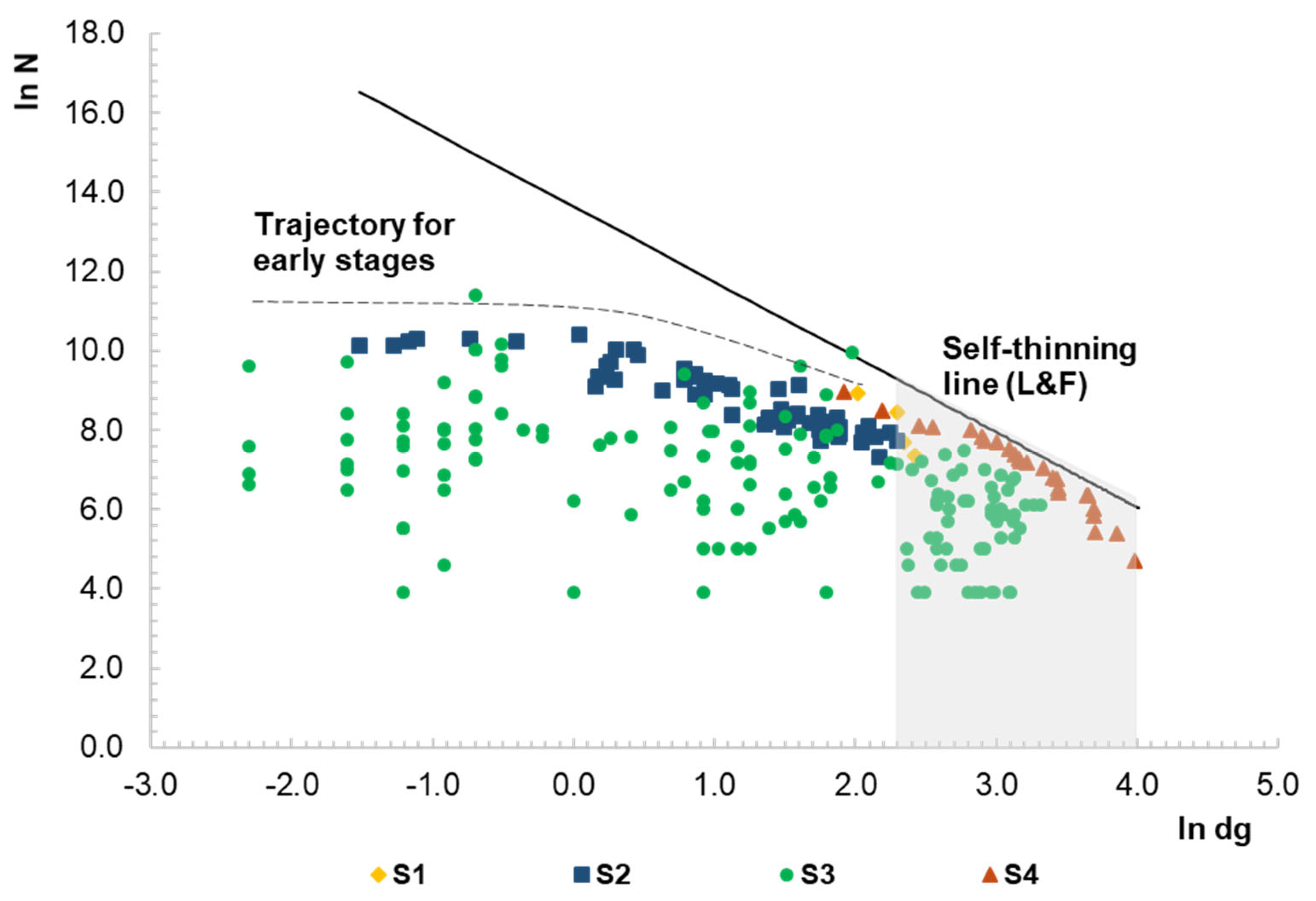
3.1. Representativeness of the Data Set and Pattern of the Density–Size Trajectory

A scattered plot for the pairs of ( d g ,     N ), transformed to logarithm values, as shown in Figure 2, reveals three different situations: a log-linear relationship for large trees (S1 and S4), a curvature of concave shape for S2, and an apparent lack of trend for the pairs of S3. Regarding the dispersion of the pairs of values, as a whole, it is noticed that they are evenly distributed along the graph region, as shown in Figure 2. The self-thinning line for maritime pine can also seen, as proposed by Luis and Fonseca [28] and hereafter termed as “L & F”, and the respective domain region in terms of average diameter range (10–50 cm), which fits closely to the S1 and S4 sampled values.
In this figure, a hand-drawn line (dashed) was placed close to the extreme pairs of size–density values registered for the young stands (S1, S2, and S3) that represents a hypothesized trajectory in the early stages of development. The size–density trajectory for maritime pine begins as a straight line parallel to the x-axis and curves toward the line L & F.

3.2. Maximum Size–Density Sample Data

The final sample of data, obtained from the filtering procedure presented in Section 2.3 applied to the original sets of data, consists of 30 observations of border points, as shown in Table 2. The border points set include 2 observations of each of the sets S1, S2, and S3, and 24 observations from the S4 database.

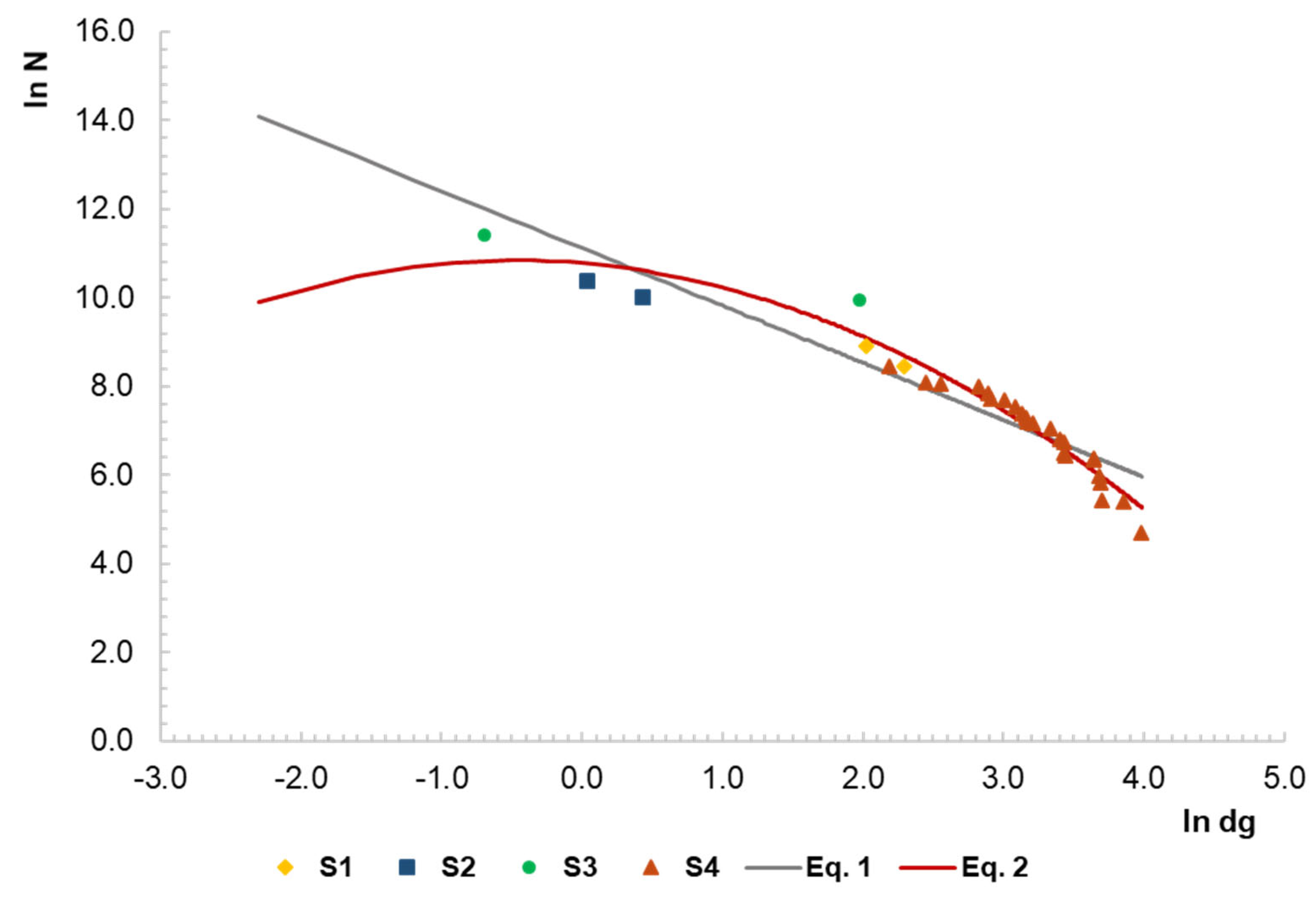
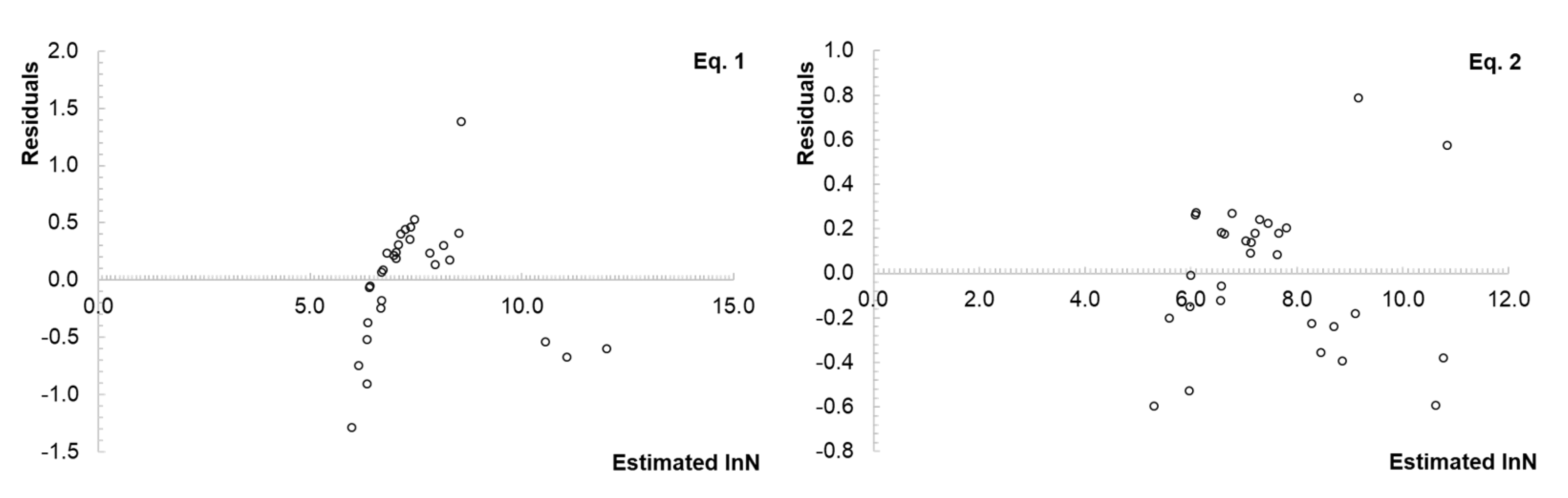
3.3. Representation of the Size–Density Pattern for the Border Points and Fitted Lines

The dispersion of the pairs ( ln d g , ln N ) retained in the final set of 30 border points is shown in Figure 3, along with the estimated models (Equations (1) and (2)), details of which are in Table 3.
The estimated parameters (and standard errors) of the regression models (Equations (1) and (2)) estimated by the least-squares regression method are significantly different from zero (p-value < 0.0001), as shown in Table 3.
The analysis of the residual for the fitted models was not clear with regard to the assumption of nonconstant error variance, as shown in Figure 4. The homoscedasticity condition was confirmed by the Spearman test for both models ( ρ = −0.155, p-value = 0.415, for Equation (1), and ρ = −0.325, p-value = 0.08, for Equation (2)). For Equation (1), a curvature occurs in the pattern of the residuals, suggesting a specification error. The goodness-of-fit statistics (R2adj) for the proposed models was higher than 88%, as shown in Table 3. The VIF value for Equation (2) was equal to or less than 5 (VIF = 3.1), implying that no severe implications of multicollinearity are expected.

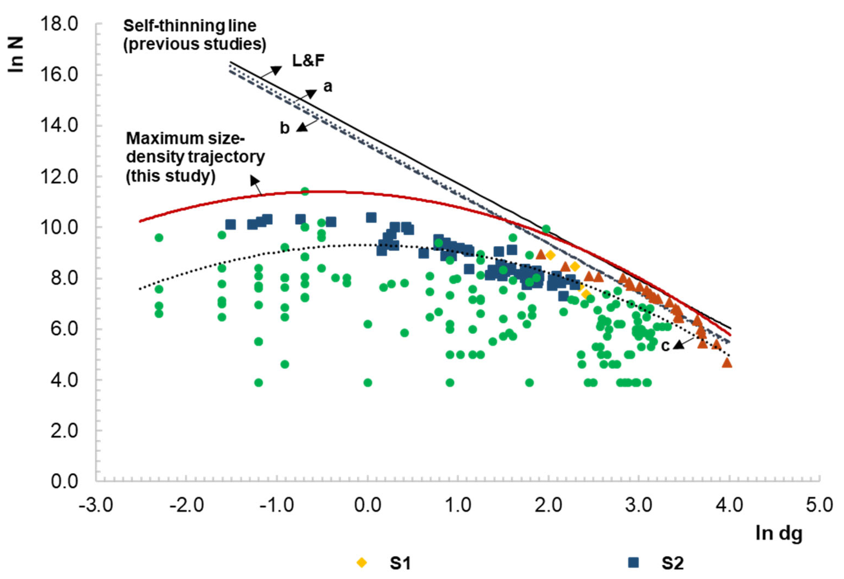
3.4. Maximum Size–Density Trajectory over All the Stages of Development

Equation (2) adequately fits the trajectory of size–density for the stands corresponding to the border points. This model represents the expected average size–density trajectory over all the stages of development. To describe a trajectory corresponding to the maximum attainable values of density for a given tree diameter, the estimated line has to be positioned above the extreme points. A logically reasonable position to allocate the curve is to raise it to the upper limit of the confidence interval for the ordinate at the origin. The upper limit was estimated as ( I n t e r c e p t + s e I n t × t ), where “ I n t e r c e p t ” is the estimate of the ordinate at the origin of the model (12.969), as shown in Table 3, “ s e I n t   “ is the statistic standard error of the intercept (0.328), as shown in Table 3, and “ t ” is the percentile of the t distribution for d f degrees of freedom. The degrees of freedom for Equation (2) are equal to the number of observations used to fit the model ( n = 30 ) minus the number of the estimated parameters ( p = 3 ). For a confidence level of 95% (unilateral) and (30 − 3) d f , the value of t is 1.703. Therefore, the upper limit of the interval for the ordinate at the origin is given by 12.969 + 0.328 × 1.703 = 13.528. The maximum size–density trajectory for maritime pine is expressed by Equation (3):
ln N = 13.528 1.832 ln d g 0.280 ( ln d g 2.796 ) 2
where N represents the number of trees per hectare (trees ha−1), and d g is the quadratic mean diameter over bark (cm) measured at the height level of 1.30 m.
For analysis purposes, the maximum density lines for the species estimated in previous studies namely by Luis and Fonseca [28], Aguirre et al. [21], Ríofrio et al. [30], and Charru et al. [26] were also considered, as shown in Figure 5, (coded as L & F, a, b, and c, respectively).

4. Discussion

4.1. Representativeness of the Database

Achieved results for young stands located in northern and central regions of Portugal (sets S2 an S3) naturally regenerated after a fire and display a variety of size–density values, which are representative of these forest systems. To the best knowledge of the authors, this is the first report of a sound database of density–size values, for the early stages of the development of the species. Previous research studies for maritime pine species rely on trees in more advanced stages of development. The domain of the self-thinning line by Luis and Fonseca [28] refers to stands with a minimum average diameter of 10 cm. Original databases from [21] and [30] report similar minimum values of pine stands (10.0–10.7 cm) with reference [26] considering upper minimum values (16 cm).
Taking into consideration the data from sets S2 and S3, the pattern of size–density values shows high variability, as shown in Figure 2, with diverse values of the number of plants reported for a given dimension. Differences might arise from the natural development of the species in naturally regenerated stands, with some pinewoods evidencing situations of understocking and other experiencing crown closure. Although the sampling plots from S2 are of a smaller size than the plots from S1, S3, and S4, there are no evident trends that might question the validity of the S2 set in terms of sampling representativeness. The values of d g ,   N from the plots sampled in the northern part of the country (S1 and S2) overlap with the values of d g ,   N evaluated in the sampling units from the stands located in the central region (S3). There is no reason for concern about a possible influence of the local in the size–density trend.
The information from S1, S2, and S3 refers to stands less than 20 years old. A sample from the NFI was added to analyze the full trajectory over all the stages of development. This sample refers to maximum size–density values filtered in the study by reference [28]. The addition of S4 to the other three sets of data enlarge the domain of the study from young to adult stands ( d g ranges from 0.5 of 53.3 cm). In terms of number of trees, the full supporting database records densities within the interval from 50 to 90,000 trees ha−1. This is a wider interval than the ones reported in the literature in concurrent studies [21,26,30].
The algorithm used for filtering the data retained the most part (24 out of 25) of the dataset S4. This high retention proportion was expected, as reference [28] previously reported these observations as border points for the species, for stands with a mean size of diameter of classes of 10 cm and higher. The additional six pairs of values ( d g ,   N ) retained from S1, S2, and S3, correspond to maximum values of density–size for the domain of values occurring at earlier stages of development, that is, occurring in the region of lower average diameter values. These values assure the continuity, in terms of database, from this domain region to the domain region covered in the study by reference [28].

4.2. Size–Density Trajectory and Self-Thinning Line

The entire database presented, as shown in Figure 2, allows for the identification of the pattern of the size–density trajectory over all the stages of development for the maritime pine species. Two trends can be noticed for increasing values of diameter. For the early stage of development, the size–density trajectory can be described as a straight line parallel to the axis representing stand size, with the uppermost limit referring to the stands under crown closure where competition modulates the maximum attainable tree number. With the increase of tree size, natural mortality driven by intraspecific competition by limited resources (light, nutrients, water) dictates a reduction in the living trees per unit of area. The horizontal trajectory moves then toward a step line, which can be modeled by a straight line or a curve, depending on the shape of the size–density trajectory being followed in the subsequent development stages.
A similar trend of a horizontal line followed by a descending line, in log-log scales, is reported for common beach stands [38], Chinese fir plantations [39], and even-aged sessile oak [40], among others. References [39] and [40] divide the full trajectory into three stages, where the second stage corresponds to a concave trajectory, and the third corresponds to a self-thinning line, describing a maximum size–density relationship that involves maximum allowable stand density for a given mean diameter.
The size–density pattern for maritime pine, as shown in Figure 2, that emerges in young stands, after crown closure, clearly represents a deviation to the extrapolated values of the number of trees obtained from the self-thinning line by Luis and Fonseca [28]. A noticeable deviation occurs at the left end, for diameters less than 10 cm. It is evident that the hypothesis of using the L & F model to describe the maximum size–density trajectory since the early stages of development after mortality onset is not adequate. The description of the maximum size–density trajectory for maritime pines requires, therefore, a reevaluation.
The continuity along the development stages could be assured by regression techniques using piecewise regression models (e.g., references [38] and [39]). Reference [39] used a nonlinear mixed-effects segment model to describe the self-thinning trajectories of Chinese fir stands in Southern China. Reference [38] proposed the use of a piecewise polynomial function to fit the trajectories of self-thinning of common beech stands in France. The methodology uses the information of initial number of trees per hectare and mean girth at breast height at the onset mortality as parameters of the trajectory model, which limits the use of the methodology to the species/cases of study where the point of onset mortality is precisely defined; when such data are not available, these techniques are not useful. Describing the line with a single function is a straightforward method, widely tested in the description of the self-thinning line with meaningful results. A major aspect to consider, with this traditional fitting approach, is the fitting of curvature in case it occurs in the domain of the range of values of ( d g ,   N ), in log-log scale.
For maritime pine, the pattern of the size–density trajectory for the border points clearly deviates from a straight line, as shown in Table 2 and Figure 3, evidencing curvature at both ends of the line. This trend is biologically expected [23] and has been reported for other species [26,27]. It occurs in young stands before the onset of competition begins, and in older stands, due to a decrease in self-tolerance [15]. Goodness-of-fit statistics for the fitted models (Equations (1) and (2)) as shown in Table 3, point out for better performance when the bend is described by a second-degree polynomial function, as shown in Table 3, (Equation (2), R2 > 0.95), instead of using the straight linear model. The description of the curvature with the three parameters of Equation (2) avoids the use of segment models or piecewise regression models, which require more parameters to estimate.
From the comparison of the self-thinning line fitted in this study and the lines defined, for the species, in previous research (i.e., references [21], [26], [28], and [30]), three evident features arise, as shown in Figure 5. The first is the goodness-of-fitting of the proposed model to the overall pattern of the ( d g ,   N ) values in log-log scale for the stands, with deviance from a straight line at both ends. The line is placed above most plots and represents the expected theoretical maximum values of the number of trees for a given diameter. The second feature is the coherence in shape with the model proposed by reference [26]. The third main feature to observe is the non-representativeness of the self-thinning lines proposed in previous studies, for the maritime pine forest systems, at early stages of development. The extrapolations to the left and of the domain for the model by reference [28] and for the models proposed for this species in Spain or in France, cannot describe the observed size–density trajectory for the species in the Portuguese forest systems. For both Spain and France, keeping the analysis under the domain of the respective models, the maximum estimated densities for diameters of 10 cm and higher (2.3 in log scale) are quite far below the values observed in even-aged pure stands of the species in Portugal.
The periods of growth considered in the self-thinning line cover the early development stage up to older stages of development. This new model represents the maximum size–density trajectory for the species and constitutes a scientifically and ecologically based support to define silvicultural guidelines for maritime pine systems regenerated after fire. Immediate applications can arise in terms of forest management. The model allows the definition of prescriptions based on a percentage of maximum density (see, for details, reference [28]). One option might be to maintain the naturally regenerated stands at high density levels (e.g., 60% of maximum) through the rotation in case aiming to promote maximum yields in short rotations. Other prescriptions are possible, depending on the aims of the management. The proposed model also applies in the management of artificial regenerated systems from young ages using the maximum attainable densities, as the theoretical limits that allow maximum volume yield.
The knowledge of the values of size–density where the stands reach and follow the self-thinning line bridges the gap in the empiricism with which these forest systems have been usually managed. Management practices should adapt and spatially diversify the structure of the forests to make them less prone to the risk of wildfires [41]. At the forest scale, typical forest management practices, such as the management of stand density [42], through thinning and harvesting systems, can contribute to reducing wildfire risk through the decrease of fuel loads [43]. These silvicultural practices can be supported by the self-thinning model proposed in the current study, serving as adaptive guidelines in the management of these pine systems. These are research directions to be considered and communicated in subsequent research under development.

5. Conclusions

A reevaluation of the self-thinning line for the maritime pine species was made, and a new model for the species was proposed. The behavior of the size–density trajectory for the initial stages of tree development and the knowledge of attainable maximum densities at the initial stage of establishment and development of natural regeneration is fundamental to identify silvicultural prescriptions and management options for the maritime pine stands. The results achieved support decision making with regard to the management of the forests originated naturally after a fire, with application also to forest systems originated artificially.

Author Contributions

Conceptualization, T.E. and T.F.; methodology, T.E., T.F., and A.C.; software, T.E., T.F., and A.C.; validation, T.F.; formal analysis, T.E., T.F., A.C., and C.A.; investigation, T.E. and T.F.; resources, C.A., J.A., and T.F.; writing—original draft preparation, T.E. and T.F.; writing—review and editing, T.E., J.L., J.T., A.C., C.A., and T.F.; supervision, T.F., J.L., J.A.; project T.F., J.A., and J.L.; funding acquisition, T.E.; J.L., J.A., A.C., C.A., and T.F.

Funding

This research was funded by the INTERACT project—‘‘Integrated Research in Environment, Agro-Chain and Technology”, No. NORTE-01-0145-FEDER-000017, in its line of research entitled BEST, co-financed by the European Regional Development Fund (ERDF) through NORTE 2020 (North Regional Operational Program 2014/2020). For authors integrated in the CITAB research center, it was further financed by the FEDER/COMPETE/POCI—Operational Competitiveness and Internationalization Programme, under Project POCI-01-0145-FEDER-006958, and by National Funds by FCT—Portuguese Foundation for Science and Technology, under the project UID/AGR/04033/2019. The participation of the co-author Teresa Fonseca was financed by the Forest Research Centre, a research unit funded by Fundação para a Ciência e a Tecnologia I.P. (FCT), Portugal (UID/AGR/00239/2019). The participation of the co-author Adelaide Cerveira was financed by National Funds through the Portuguese funding agency, FCT-Fundação para a Ciência e Tecnologia, within project: UID/EEA/50014/2019. The participation of the co-author Cristina Alegria was supported by CERNAS-IPCB [UID/AMB/00681/2019 funding by FCT].

Conflicts of Interest

The authors declare no conflict of interest.

References

  1. Doerr, S.H.; Santin, C. The ‘wildfire problem’: Perceptions and realities in a changing world. Philos. Trans. R. Soc. Lond. B. Biol. Sci. 2016, 371, 1–10. [Google Scholar] [CrossRef] [PubMed]
  2. ICNF. I F N 6—Áreas dos Usos do Solo e das Espécies Florestais de Portugal Continental 1995–2005–2010. Resultados Preliminares. 2013. Available online: https://doi.org/10.1016/j.rasd.2006.07.002 (accessed on 11 January 2019).
  3. Verkerk, P.J.; Martinez de Arano, I.; Palahí, M. The bio-economy as an opportunity to tackle wildfires in Mediterranean forest ecosystems. For. Policy Econ. 2018, 86, 1–3. [Google Scholar] [CrossRef]
  4. AFN. FloreStat, 5th National Forest Inventory Information Retrieval Tool; Ministério da Agricultura, do Desenvolvimento Rural e das Pescas: Lisboa, Portugal, 2010; Available online: http://www2.icnf.pt/portal/florestas/ifn/ifn5/rel-fin (accessed on 26 January 2018).
  5. DR, Resolução do Conselho de Ministros n° 114/2006, Estratégia Nacional Para as Florestas. Diário da República, I Série—n° 179 de 15 de Setembro 2006. Available online: http://www.dre.pt/pdf1s/2006/07/13800/50145029.pdf (accessed on 20 April 2018).
  6. Fernandes, P.M.; Rigolot, E. The fire ecology and management of maritime pine (Pinus pinaster Ait.). For. Ecol. Manag. 2007, 241, 1–13. [Google Scholar] [CrossRef]
  7. Freitas, T.M.D. Avaliação da Biomassa em Regeneraçã de Pinheiro Bravo Pós Fogo; Final Project Report; UTAD: Vila Real, Portugal, 2013; p. 57. [Google Scholar]
  8. Rodrigues, M.R.C. Análise Multi-Temporal de Crescimento de Espécies Florestais. Criação de um SIG Para a Sua Gestão. Master Thesis, Universidade de Trás-os-Montes e Alto Douro, Vila Real, Portugal, 2008. [Google Scholar]
  9. Alegria, C.; Pedro, N.; do Carmo Horta, M.; Roque, N.; Fernandez, P. Ecological envelope maps and stand production of eucalyptus plantations and naturally regenerated maritime pine stands in the central inland of Portugal. For. Ecol. Manag. 2019, 432, 327–344. [Google Scholar] [CrossRef]
  10. Calvo, L.; Santalla, S.; Valbuena, L.; Marcos, E.; Tárrega, R.; Luis-Calabuig, E. Post-fire natural regeneration of a Pinus pinaster forest in NW Spain. Plant Ecol. 2008, 197, 81–90. [Google Scholar] [CrossRef]
  11. Tapias, R.; Climent, J.; Pardos, J.A.; Gil, L. Life histories of Mediterranean pines. Plant. Ecol. 2004, 171, 53–68. [Google Scholar] [CrossRef]
  12. Martínez-Sánchez, J.J.; Marin, A.; Herranz, J.P.; Ferrandis, P.; De las Heras, J. Effects of high temperatures on germination of Pinus halepensis Mill. and P. pinaster Aiton subsp, pinaster seeds in southeast Spain. J. Vegetatio 1995, 116, 69–72. [Google Scholar]
  13. Moya, D.; Espelta, J.M.; López-Serrano, F.R.; Eugenio, M.; Heras, J.D. Natural post-fire dynamics and serotiny in 10-year-old Pinus halepensis Mill. stands along a geographic gradient. Int. J. Wildl. Fire 2008, 17, 287–292. [Google Scholar] [CrossRef]
  14. Maia, P.; Keizer, J.; Vasques, A.; Abrantes, N.; Roxo, L.; Fernandes, P.; Ferreira, A.; Moreira, F. Post-fire plant diversity and abundance in pine and eucalypt stands in Portugal: Effects of biogeography, topography, forest type and post-fire management. For. Ecol. Manag. 2014, 334, 154–162. [Google Scholar] [CrossRef]
  15. Zeide, B. Analysis of the 3/2 Power Law of Self-Thinning. For. Sci. 1987, 33, 517–537. [Google Scholar]
  16. Reineke, L.H. Perfecting a stand-density index for even-aged forests. J. Agric. Res. 1933, 46, 627–638. [Google Scholar]
  17. Yoda, K. Self-thinning in overcrowded pure stands under cultivated and natural conditions (Intraspecific competition among higher plants. XI). J. Inst. Polytech. Osaka City Univ. Ser. D 1963, 14, 107–129. [Google Scholar]
  18. Harper, J.L. Population Biology of Plants; Academic Press: Cambridge, MA, USA, 1977; ISBN 9780123258526. [Google Scholar]
  19. Brunet-Navarro, P.; Sterck, F.J.; Vayreda, J.; Martinez-Vilalta, J.; Mohren, G.M.J. Self-thinning in four pine species: An evaluation of potential climate impacts. Ann. For. Sci. 2016, 73, 1025–1034. [Google Scholar] [CrossRef]
  20. Panayotov, M.; Kulakowski, D.; Tsvetanov, N.; Krumm, F.; Berbeito, I.; Bebi, P. Climate extremes during high competition contribute to mortality in unmanaged self-thinning Norway spruce stands in Bulgaria. For. Ecol. Manag. 2016, 369, 74–88. [Google Scholar] [CrossRef]
  21. Aguirre, A.; del Río, M.; Condés, S. Intra- and inter-specific variation of the maximum size-density relationship along an aridity gradient in Iberian pinewoods. For. Ecol. Manag. 2018, 411, 90–100. [Google Scholar] [CrossRef]
  22. Andrews, C.; Weiskittel, A.; D’Amato, A.W.; Simons-Legaard, E. Variation in the maximum stand density index and its linkage to climate in mixed species forests of the North American Acadian Region. For. Ecol. Manag. 2018, 417, 90–102. [Google Scholar] [CrossRef]
  23. Zeide, B. A relationship between size of trees and their number. For. Ecol. Manag. 1995, 72, 265–272. [Google Scholar] [CrossRef]
  24. Cao, Q.V.; Dean, T.J.; Baldwin, V.C. Modeling the size-density relationship in direct-seeded Slash pine stands. For. Sci. 2000, 46, 317–321. [Google Scholar]
  25. Monserud, R.A.; Ledermann, T.; Sterba, H. Are self-thinning constraints needed in a tree-specific mortality model? For. Sci. 2005, 50, 848–858. [Google Scholar]
  26. Charru, M.; Seynave, I.; Morneau, F. Significant differences and curvilinearity in the self-thinning relationships of 11 temperate tree species assessed from forest inventory data. Ann. For. Sci. 2012, 69, 195–205. [Google Scholar] [CrossRef]
  27. Fonseca, T.; Monteiro, L.; Enes, T.; Cerveira, A. Self-thinning dynamics in cork oak woodlands: Providing a baseline for managing density. For. Syst. 2017, 26, 1–10. [Google Scholar] [CrossRef]
  28. Luis, J.S.; Fonseca, T.F. The allometric model in the stand density management of Pinus pinaster Ait. in Portugal. Ann. For. Sci. 2004, 61, 807–814. [Google Scholar] [CrossRef]
  29. Fonseca, T.; Parresol, B.; Marques, C.; de Coligny, F. Models to Implement a Sustainable Forest Management—An Overview of the ModisPinaster Model. In Sustainable Forest Management/Book 1; Martín García, J., Diez Casero, J.J., Eds.; InTech—Open Access Publisher: Rijeka, Croatia, 2012; pp. 321–338. ISBN 978-953-51-0621-0. [Google Scholar]
  30. Riofrío, J.; Del Río, M.; Bravo, F. Mixing effects on growth efficiency in mixed pine forests. Forestry 2017, 90, 381–392. [Google Scholar] [CrossRef]
  31. Rivas-Martinez, S.; Fernández-González, F.; Loidi, J.; Lousa, M.; Penas, A. Vascular plant communities of Spain and Portugal. Addenda to the syntaxonomical checklist of 2001. Part II. In Itinera Geobotanica; Leon, Spain, 2002; Volume 15, ISSN 0213-8530. Available online: https://webs.ucm.es/info/cif/book/addenda/addenda1_00.htm (accessed on 13 November 2018).
  32. SNIRH. Sistema Nacional de Informação de Recursos Hídricos. Available online: http://www.snirh.pt (accessed on 13 November 2018).
  33. Marques, C.P. Evaluating site quality of even-aged maritime pine stands in northern Portugal using direct and indirect methods. For. Ecol. Manag. 1991, 41, 193–204. [Google Scholar] [CrossRef]
  34. Fonseca, T.J.F. Modelação do Crescimento, Mortalidade e Distribuição Diamétrica, do Pinhal Bravo no Vale do Tâmega. Ph.D. Thesis, Universidade de Trás-os-Montes e Alto Douro, Vila Real, Portugal, 2004. [Google Scholar]
  35. Keeney, R.; Raiffa, H.; Rajala, D. Decisions with Multiple Objectives: Preferences and Value Trade-Offs. Syst. Man Cybern. IEEE Trans. 1979, 9, 403. [Google Scholar] [CrossRef]
  36. Neter, J.; Kutner, M.; Nachtsheim, C.; Wassermaniption, W. Applied Linear Statistical Models, 3rd ed.; Irwin: Chicago, IL, USA, 1996. [Google Scholar]
  37. Myers, R.H. Classical and Modern Regression with Applications; Duxbury advanced series in statistics and decision sciences; PWS-KENT: Belmont, CA, USA, 1990; ISBN 9780534922412. [Google Scholar]
  38. Ningre, F.; Ottorini, J.M.; Le Goff, N. Modeling size-density trajectories for even-aged beech (Fagus silvatica L.) stands in France. Ann. For. Sci. 2016, 73, 765–776. [Google Scholar] [CrossRef]
  39. Zhang, X.; Cao, Q.V.; Duan, A.; Zhang, J. Self-thinning trajectories of Chinese fir plantations in Southern China. For. Sci. 2016, 62, 594–599. [Google Scholar] [CrossRef]
  40. Ningre, F.; Ottorini, J.-M.; Le Goff, N. Size-density trajectories for even-aged sessile oak (Quercus petraea (Matt.) Liebl.) and common beech (Fagus sylvatica L.) stands revealing similarities and differences in the mortality process. Ann. For. Sci. 2019, 76, 73. [Google Scholar] [CrossRef]
  41. Lauer, C.J.; Montgomery, C.A.; Dietterich, T.G. Spatial interactions and optimal forest management on a fire-threatened landscape. For. Policy Econ. 2017, 83, 107–120. [Google Scholar] [CrossRef]
  42. Fonseca, T.F.; Duarte, J.C. A silvicultural stand density model to control understory in maritime pine stands. iForest 2017, 10, 829–836. [Google Scholar] [CrossRef]
  43. Fernandes, P.M. Fire-smart management of forest landscapes in the Mediterranean basin under global change. Landsc. Urban. Plan. 2013, 110, 175–182. [Google Scholar] [CrossRef] [Green Version]
Figure 1. Graphical representation of potential frontier points in the objective space (dg, N).
Forests 10 01057 g001
Figure 2. Diagram of dispersion and relationship between the logarithm of N (trees.ha−1) and the logarithm of quadratic mean diameter (dg (cm)), for the observations of the four data subsets. Two lines are imposed: the estimated maximum size–density values according to the allometric model by Luis and Fonseca [28] (L & F), and a hypothesized line (hand-drawn, dashed) placed close to the extreme pairs of (dg, N) values registered for the young stands. The shaded area represents the domain region of the L & F model, for the diameter variable.
Forests 10 01057 g002
Figure 3. Diagram of dispersion and relationship between the logarithm of N (trees.ha−1) and the logarithm of dg (cm) for the dataset of 30 border points. The straight line corresponds to the fitted linear model (Equation (1)) and the curve to the quadratic model (Equation (2)).
Forests 10 01057 g003
Figure 4. Plots of the residuals for the fitted linear model (Equation (1)) and the quadratic model (Equation (2)).
Forests 10 01057 g004
Figure 5. Size–density trajectories for maritime pine as defined in previous research (L & F—Luis and Fonseca [28]; a—Aguirre et al. [21]; b—Ríofrio et al. [30]; c—Charru et al. [26]) and in the current study—line in red. The points represented in the graph refer to the four data subsets.
Forests 10 01057 g005
Table 1. Summary characteristics of the number of trees per hectare (N) and quadratic mean diameter (dg) for the sampled plots of maritime pine.
SourcenN (trees.ha−1)dg (cm)
MinMeanMaxsdMinMeanMaxsd
S1415603985750027087.59.811.21.6
S2591500953632,50085490.24.09.92.6
S315350309190,00084600.18.027.58.0
S4251101724768017056.827.253.312.0
Legend: n—number of plots/observations; N—number of trees per hectare (trees.ha−1); dg—quadratic mean diameter measured at the height level of 1.30 m; Min—data minimum; Mean—data average; Max—data maximum; and sd—data standard deviation.
Table 2. Summary characteristics of the data used in the self-thinning line estimation.
SourcenN (trees.ha−1)dg (cm)
MinMeanMaxsdMinMeanMaxsd
Border points30110712190,00017,3660.523.353.314.1
Legend: n—number of plots/observations; N—number of trees per hectare (trees.ha−1); dg—quadratic mean diameter measured at the height level of 1.30 m; Min—data minimum; Mean—data average; Max—data maximum; and sd—data standard deviation.
Table 3. Coefficients (standard errors) and fit statistics of the estimated models to support the definition of the maximum size–density trajectory for maritime pine (n = 30 observations). RMSE: root mean square error.
Model (Equation)Estimates (Stand Error) Fit Statistics
Interceptrs l n d g ¯ R2adjRMSE
Equation (1)11.115 (0.270)−1.290 (0.090)--0.8760.541
Equation (2)12.969 (0.328)−1.832 (0.100)−0.280 (0.042)2.7960.9540.341

