An Objective Function-Based Clustering Algorithm with a Closed-Form Solution and Application to Reference Interval Estimation in Laboratory Medicine

Abstract

Clustering algorithms are usually iterative procedures. In particular, when the clustering algorithm aims to optimise an objective function like in k-means clustering or Gaussian mixture models, iterative heuristics are required due to the high non-linearity of the objective function. This implies higher computational costs and the risk of finding only a local optimum and not the global optimum of the objective function. In this paper, we demonstrate that in the case of one-dimensional clustering with one main and one noise cluster, one can formulate an objective function, which permits a closed-form solution with no need for an iteration scheme and the guarantee of finding the global optimum. We demonstrate how such an algorithm can be applied in the context of laboratory medicine as a method to estimate reference intervals that represent the range of “normal” values.

1. Introduction

Cluster analysis is often characterised as methods for partitioning data into homogeneous groups called clusters or hidden classes [1,2,3]. Although this idea of clustering to partition data into well-separated groups is appealing and commonly accepted, cluster analysis is often (mis-)used for other purposes like pure partitioning without the requirement of separateness or—in the extreme case—for outlier detection where the presence of actual clusters or their structures becomes completely unimportant because only single outlier points are of interest, as in [4]. In this paper, we will focus on a scenario where we are only interested in finding a single cluster. Nevertheless, applying such an algorithm in a repeated manner by removing each time the identified cluster from the data can also be used to find multiple clusters. This strategy is also called subtractive clustering.

As mentioned before, cluster analysis is usually viewed as a data partitioning task to discover hidden or latent classes. Clustering is therefore very popular as a central approach in many applications where a hidden structure is suspected in a dataset [5] with applications in almost all fields ranging from engineering [6] to social economics and education [7].

Validity measures or indices for the evaluation of clustering results reflect the idea of finding more or less distinct clusters with homogeneity within each cluster and high heterogeneity between different clusters [8]. In particular, internal indices, which are based on the data to be clustered, focus on these properties [9], whereas external validation measures use other external properties provided about the data [10].

As an application example for our clustering algorithm, we consider measurements in laboratory medicine where reference intervals play a crucial role. A reference interval for an analyte like haemoglobin represents the “normal range” representing the central 95% of a healthy cohort. Indirect methods for the determination of reference intervals use all measurements for an analyte and try to separate the main cluster of non-pathological values from pathological values. Therefore, the focus here is to identify a single cluster in a dataset and to separate it from the remaining “noise” data. Because we are not interested in finding all clusters, we do not apply internal validation measures, but external ones in the sense of comparing the computed reference intervals with theoretical ones in the case of synthetic data and with reference intervals from other algorithms in the case of real data.

One way to approach cluster analysis is a purely algorithmic one, i.e., one defines an algorithm that joins data points together to clusters by reasonable criteria. Hierarchical clustering is probably the most popular algorithm in this class. The closest data points are joined together to clusters step by step. Density-based clustering algorithms like DBSCAN (density-based spatial clustering of applications with noise) [11] or its extension, OPTICS (ordering points to identify the clustering structure) [12], fall into the same class. They find regions of high data density step-by-step to define clusters. Neural network-based self-organising maps [13] fall also into this class of algorithms and adjust feature vectors representing the clusters in an iterative manner.

Other clustering algorithms are based on an objective function, which measures how well a clustering fits the data. A very simple and popular representative of this class of clustering methods is the k-means algorithm. The algorithm tries to minimise the squared distances between data points and their cluster centres by greedy heuristics that optimise the locations of the cluster centres and the assignment of the data to the cluster in an alternating fashion based on a random or “clever” initialisation [14], leading to an iterative greedy algorithm that is prone to being stuck in local minima. Fuzzy clustering generalises the dichotomous assignments to clusters by membership degrees between 0 and 1 and adapts the alternating optimisation scheme to a corresponding modified objective function.

Mixture models interpret the clusters as multivariate—e.g., Gaussian—probability distributions, and aim to maximise the likelihood for the data using the EM (expectation maximisation) algorithm [15], which is also a greedy alternating optimisation strategy.

Even the simple k-means setting belongs to the class of NP-hard problems [16], so there is probably no other way than using a heuristic strategy to optimise its objective function. Nevertheless, there are various attempts to design single-pass clustering algorithms, see, for instance, [17,18], especially in the context of data stream clustering [19], where the price for the acceleration is often an inferior local optimum of the objective function.

Because even the simple k-means problem is NP-hard, there is little hope of finding closed-form solutions for the global optimum of the objective function for more sophisticated algorithms in a general setting. However, for specific cluster analysis problems with further restricting assumptions, it can be possible to derive closed-form solutions yielding single-pass algorithms with a guarantee to find the global optimum. Here, we consider such a specific clustering setting where we can derive a closed-form solution. Section 2 provides the technical and formal background on which our algorithm is based. Section 3 describes the specific clustering problem we consider and derives the closed-form solution for the optimum of the objective function. Limitations, parameter settings, and an extension of the algorithm are discussed in Section 4. An application to so-called indirect reference interval estimation in laboratory medicine is illustrated in Section 5 before we conclude the paper with a discussion in Section 6.

2. Fuzzy and Noise Clustering

The k-means clustering algorithm requires as input a dataset $\{x_1,\dots ,x_n\}\subset {\mathbb{R}}^q$. Assuming a predefined number of clusters k, the algorithm tries to minimise the objective function, as follows:

$$f=\sum _{i=1}^k\sum _{j=1}^n{u}_{ij}{d}_{ij}$$

(1)

under the constraints

$$\sum _{i=1}^k{u}_{ij}=1\mathrm{for} \mathrm{all} j\in \{1,\dots ,n\}$$

(2)

where $u_{ij}\in \{0,1\}$ indicates whether data point $x_j$ is assigned to cluster i ($u_{ij}=1$) or not ($u_{ij}=0$). $d_{ij}={\Vert x_j-v_i\Vert }^2$ denotes the squared Euclidean distance between data point $x_j$ and cluster centre $v_i$. As already mentioned before, the k-means algorithm tries to solve an NP-hard problem [16], which is a mixed discrete and continuous optimisation problem. The assignment of the data points to the clusters is a discrete problem whereas the estimation of the cluster centres is a continuous problem.

Fuzzy clustering turns the mixed optimisation problem into a purely continuous one by relaxing the constraint $u_{ij}\in \{0,1\}$ to $u_{ij}\in [0,1]$. It is, however, quite easy to see that the optimum of the objective function with the relaxed constraint is still found at the margins, i.e., for the optimum $u_{ij}\in \{0,1\}$ will hold although intermediate values are permitted. The simple reason is that for a data point, there is no benefit in assigning any share of its membership degree to a cluster centre that is not closest to the data point, as this would obviously increase the value of the objective function. There are essentially two different strategies to avoid the problem [20]. One way is the “fuzzification” of the membership transformation, i.e., to modify the linear weighting with the membership degrees $u_{ij}$ in Equation (1) to

$$f=\sum _{i=1}^k\sum _{j=1}^{n}h\left(u_{ij}\right)d_{ij}$$

(3)

with a suitable non-linear function, h. The most common function, h, is $h\left(u\right)=u^2$[21], or its generalisation, $h\left(u\right)=u^m$, with the so-called fuzzifier, $m>1$ [22].

The alternative is to keep the linear weighting with the membership degrees and to introduce a regularisation term instead that punishes the values 0 and 1 by

$$f=\sum _{i=1}^k\sum _{j=1}^n{u}_{ij}{d}_{ij}+\alpha \sum _{i=1}^k\sum _{j=1}^{n}g\left(u_{ij}\right)$$

(4)

with a suitable convex function, g, on the unit interval. The parameter $\alpha$ controls the penalty for membership degrees of 0 and 1. For $\alpha =0$, one obtains the original k-means objective function. The larger the $\alpha$, the more the membership degrees are pushed away from 0 and 1. As pointed out in [20], Daróczy entropy [23] provides a number of example functions for g, leading to an approach that is very closely related to the EM algorithm [24]. In Section 3, the approach in Equation (4) will be used with a specific choice of the function g and the introduction of a so-called noise cluster.

The idea of noise clustering goes back to Davé [25] who introduced an additional cluster without a cluster centre or any other parameter to be optimised. Instead, the noise cluster has a fixed large predefined distance $\delta$ to all data points. In this way, this noise cluster collects all points lying far away from all other clusters or cluster centres.

3. Derivation of the Algorithm

We consider the objective function (4) that should be minimised under the following constraints:

$$\sum _{i=1}^k{u}_{ij}=1\mathrm{for} \mathrm{all} j\in \{1,\dots ,n\}$$

(5)

and

$$u_{ij}\ge 0\mathrm{for} \mathrm{all} i\in \{1,\dots ,k\} \mathrm{and} \mathrm{for} \mathrm{all} j\in \{1,\dots ,n\}$$

(6)

where $u_{ij}$ indicates how much data point $x_j$ is assigned to cluster i. $d_{ij}={\Vert x_j-v_i\Vert }^2$ is the squared Euclidean distance between data point $x_j$ and cluster centre $v_i$.

The second term in Equation (4) should reward non-crisp membership degrees, i.e., values greater than zero but smaller than one. For this purpose, we require that the function $g:[0,1]\to \mathbb{R}$ be twice differentiable and that $g^{\prime \prime }\left(x\right)>0$ holds. The parameter $\alpha$ controls the extent to which membership degrees deviating from zero and one are rewarded.

The corresponding Lagrange function for this optimisation problem is as follows:

$$f_{\mathrm{Lagrange}}=\sum _{i=1}^k\sum _{j=1}^n{u}_{ij}{d}_{ij}+\alpha \sum _{i=1}^k\sum _{j=1}^{n}g\left(u_{ij}\right)+\sum _{j=1}^n{\lambda }_j\left(1-\sum _{i=1}^k{u}_{ij}\right).$$

(7)

The partial derivative with respect to $u_{ij}$ is then

$$\frac{\partial f_{\mathrm{Lagrange}}}{\partial u_{ij}}=d_{ij}+\alpha ·g^{\prime }\left(u_{ij}\right)-{\lambda }_j=0$$

(8)

for all $i\in \{1,\dots ,k\}$ and for all $j\in \{1,\dots ,n\}$. This implies

$${\lambda }_j=d_{ij}+\alpha ·g^{\prime }\left(u_{ij}\right)=d_{rj}+\alpha ·g^{\prime }\left(u_{rj}\right)$$

(9)

for $i,r\in \{1,\dots ,k\}$, $i\ne r$.

For the special case of $g^{\prime }\left(x\right)=x$, i.e., $g\left(x\right)=\frac{x^2}{2}$, we obtain the following:

$$u_{rj}=\frac{d_{ij}-d_{rj}}{\alpha }+u_{ij}$$

(10)

implying

$$1=\sum _{r=1}^k{u}_{rj}=\frac{k·d_{ij}-{\sum }_{r=1}^k{d}_{rj}}{\alpha }+k·u_{ij}$$

(11)

leading to

$$u_{ij}=\frac{1}{k}+\frac{\frac{1}{k}\left({\sum }_{r=1}^k{d}_{rj}\right)-d_{ij}}{\alpha }.$$

(12)

Equation (12) can lead to negative values for $u_{ij}$, violating constraint (6). One can either choose $\alpha$ sufficiently large so that $u_{ij}\ge 0$ is always guaranteed or one has to remove, step by step, the largest negative $u_{ij}$ and simultaneously reduce the number of clusters, k, in Equation (12), in a similar manner as in [26].

We now restrict the problem to one single cluster and a noise cluster, meaning that we have only two membership degrees for each data point, i.e., the membership degrees to the single cluster and the noise cluster. Such an approach can be used to identify a main cluster as in Section 5 or to apply a subtractive clustering strategy removing single clusters step by step [27,28,29]. Assuming a sufficiently large $\alpha$, Equation (12) simplifies to the following:

$$u_j=\frac{1}{2}+\frac{\delta -d_j}{2\alpha }$$

(13)

where $u_j$ is the membership degree of data point $x_j$ to the single cluster and $\delta$ is the (squared) noise distance. The membership degree of data point $x_j$ to the noise cluster is $1-u_j$.

In the one-dimensional case, Equation (4) is as follows:

$$\begin{array}{ccc}\hfill f\left(x\right)& =& \sum _{j=1}^n\left(u_j{(x_j-x)}^2+(1-u_j)\delta +\alpha \left(\frac{u_j^2}{2}+\frac{{(1-u_j)}^2}{2}\right)\right)\hfill \\ \hfill & =& \sum _{j=1}^n\left(u_j\left({(x_j-x)}^2-\delta \right)+\delta +\alpha u_j^2-\alpha u_j+\frac{\alpha }{2}\right)\hfill \\ \hfill & =& \left(\sum _{j=1}^n{u}_j\left(\alpha u_j+{(x_j-x)}^2-\delta -\alpha \right)\right)+n\delta +\frac{n\alpha }{2}\hfill \\ \hfill & =& \left[\sum _{j=1}^n\left(\frac{1}{2}+\frac{\delta -{(x_j-x)}^2}{2\alpha }\right)\left(\alpha \left(\frac{1}{2}+\frac{\delta -{(x_j-x)}^2}{2\alpha }\right)+{(x_j-x)}^2-\delta -\alpha \right)\right]\hfill \\ \hfill & & +n\delta +\frac{n\alpha }{2}.\hfill \end{array}$$

(14)

i.e., it is a fourth-degree equation in the cluster centre, x, so that the derivative is a cubic equation in x.

Taking the derivative of Equation (4) yields the following:

$$f^{\prime }\left(x\right)=\frac{1}{\alpha }\sum _{j=1}^n\left(x_j^3-\alpha x_j-\delta x_j+(\alpha +\delta -3x_j^2)x+3x_j{x}^2-x^3\right)=0.$$

(15)

This cubic equation, which can be solved by Cardano’s formula, should have (up to) three real solutions. Because the coefficient of $x^3$ is negative, this implies that the coefficient of $x^4$ in Equation (4) is negative, meaning that Equation (4) goes to $-\infty$ for $x\to \pm \infty$. Therefore, the three real solutions of the derivative should correspond to two local maxima and one local minimum between the two local maxima. This local minimum is the solution we are looking for. The global minimum of Equation (14) is at $\pm \infty$, i.e., moving the cluster centre to infinity. This would, however, imply that the membership degrees to the cluster become negative according to Equation (13).

Algorithm 1 describes the basic clustering algorithm, which only works if $\alpha$ is chosen sufficiently large. The problem of $\alpha$ being too small will be discussed in the next section.

Algorithm 1 Basic clustering algorithm
1: procedure oneCluster($x,\delta ,\alpha$)	▹ Input $x\in {\mathbb{R}}^n$ values to be clustered
2:	▹$\delta >0$ noise distance, $\alpha >0$ (see Equation (4))
3:      $(y_1,y_2,y_3)\leftarrow$ Cardano (Equation (15))	▹ Roots of Equation (15), $y_1<y_2<y_3$
4:	▹$y_2$ is the cluster centre.
5:      for $i\in \{1,\dots ,n\}$ do	▹ Compute membership degrees according to
6:          $u_j\leftarrow \frac{1}{2}+\frac{\delta -{(x_j-y_2)}^2}{2\alpha }$	▹ Equation (13)
7:      end for
8:      return $y_2,u_1,\dots ,u_n$	▹ Cluster centres and membership degrees
9: end procedure

4. Properties of the Algorithm and Its Extensions

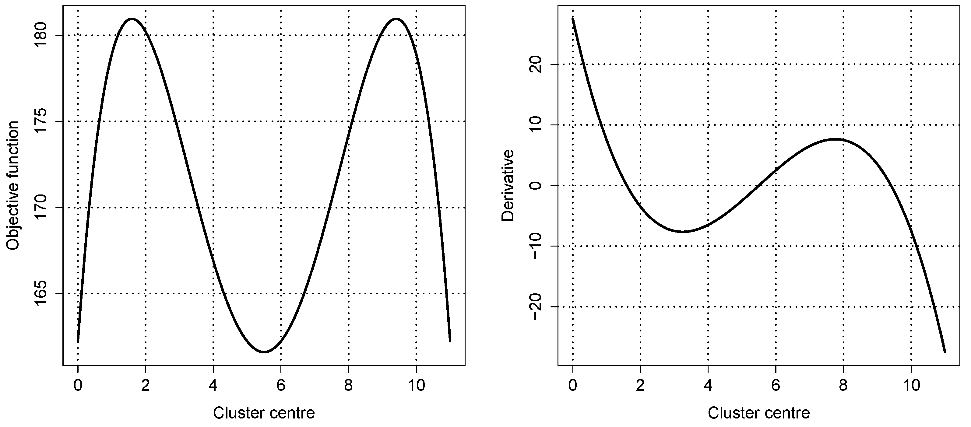
For the derivation of Algorithm 1, the constraint $u_j\in [0,1]$ was not incorporated in the derivation, and according to Equation (13), it is also possible that negative values or values larger than 1 are possible for $u_j$ if $\alpha$ is not chosen sufficiently large. For illustration purposes, we consider the simple dataset, $\{1,2,3,\dots ,10\}$. Figure 1 shows the objective function (left) and its derivative (right) for this dataset with the parameter settings $\delta =10$ and $\alpha =30$. It should be noted that $\delta$ must be interpreted as the squared noise distance.

One can easily identify the two local maxima and the local minimum in between the objective function and the corresponding roots of the derivative. Due to the construction of the dataset, the local minimum of the objective function—the cluster centre—is at 5.5 and the curve is symmetric with respect to this point. In this case, $\alpha$ is sufficiently large, resulting in only positive membership degrees.

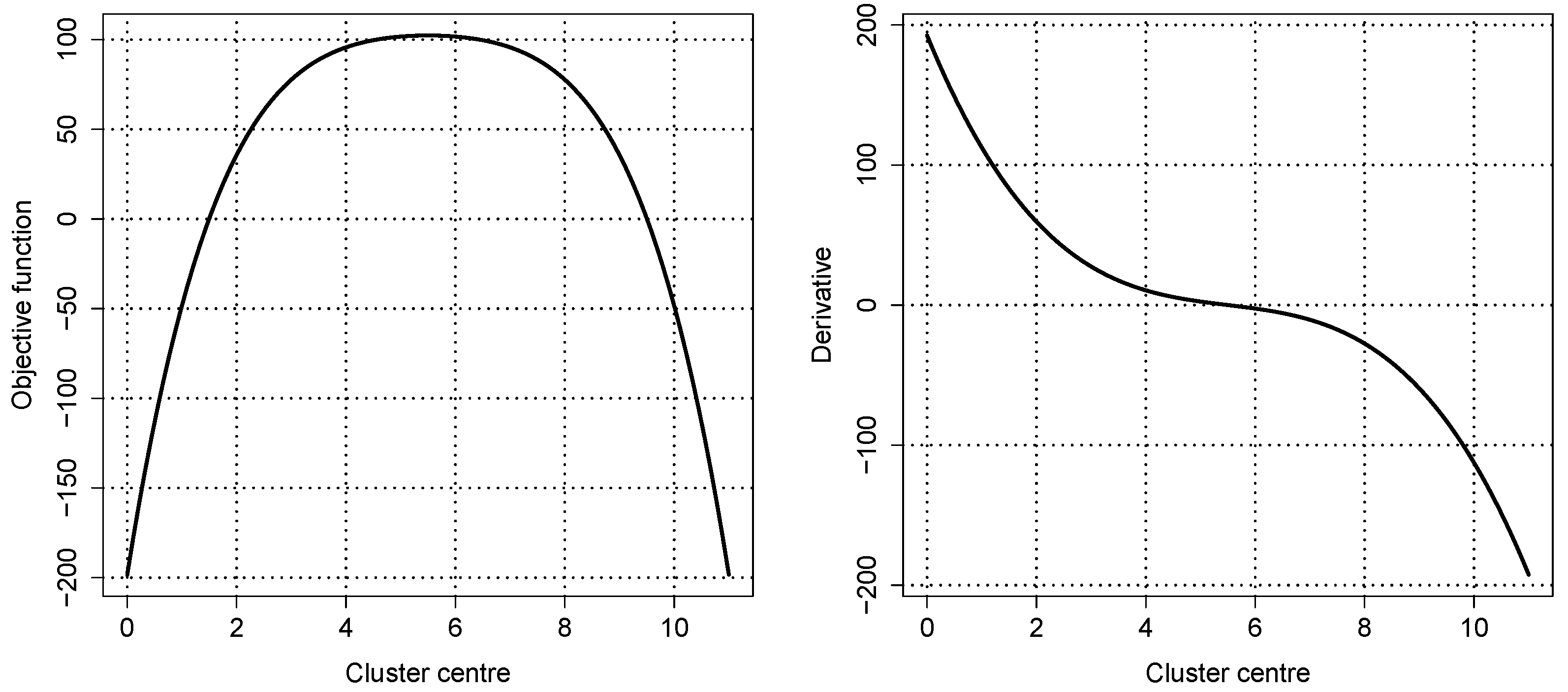
For Figure 2, $\alpha$ was changed to the smaller, value $\alpha =10$. In this case, $\alpha$ is too small, and the local minimum of the objective function vanishes while the two local maxima are joined together. The derivative has only one real root. Computing the membership degrees with the cluster centre at 5.5, Equation (13) yields partly negative values. In this case, Algorithm 1 would fail because it relies on three different real roots of the derivative of the objective function.

To amend this problem, we modify Algorithm 1 by checking whether the derivative in Equation (15) has three different real roots. If not, $\alpha$ is increased step by step by a constant factor until it is large enough to produce three different real roots for Equation (15). Algorithm 2 describes this modified version in detail.

Algorithm 2 Modified clustering algorithm
1: procedure oneClusterMod($x,\delta ,\alpha$)	▹ Input $x\in {\mathbb{R}}^n$ values to be
2:	▹ clustered, $\delta >0$ noise distance, $\alpha >0$ (see Equation (4))
3:      $c\leftarrow 1.1$	▹ Factor for increasing $\alpha$
4:      $(y_1,y_2,y_3)\leftarrow$ Cardano (Equation (15))	▹ Roots of Equation (15)
5:      has3roots $\leftarrow (y_1,y_2,y_3\in \mathbb{R}\wedge y_1\ne y_2\ne y_3\ne y_1)$
6:      while !has3roots do
7:          $\alpha \leftarrow c·\alpha$
8:          $(y_1,y_2,y_3)\leftarrow$ Cardano (Equation (15))
9:          has3roots $\leftarrow (y_1,y_2,y_3\in \mathbb{R}\wedge y_1\ne y_2\ne y_3\ne y_1)$
10:      end while
11:      for $i\in \{1,\dots ,n\}$ do	▹ Compute membership degrees according to
12:          $u_j\leftarrow \frac{1}{2}+\frac{\delta -{(x_j-y_2)}^2}{2\alpha }$	▹ Equation (13)
13:      end for
14:      return $y_2,\alpha ,u_1,\dots ,u_n$
15: end procedure

Instead of using the iterative procedure for the adjustment of the parameter $\alpha$, one could also use a “worst case scenario” for $\alpha$ to guarantee that membership degrees are between 0 and 1. For a given value of $\delta$, Equation (13) satisfies the constraint $0\le u_j\le 1$ if and only if

$$\left|\frac{\delta -d_j}{2\alpha }\right|\le \frac{1}{2}$$

(16)

holds for all $j\in \{1,\dots ,n\}$ or, equivalently

$$\alpha \ge \underset{j\in \{1,\dots ,n\}}{\max }\left|\delta -d_j\right|.$$

(17)

Because $d_j$ is the squared distance to the cluster centre, which must not lie between the smallest and largest data point, Equation (17) is satisfied if

$$\alpha \ge \max \left\{\delta ,{\left(\max \{x_1,\dots ,x_n\}-\min \{x_1,\dots ,x_n\}\right)}^2-\delta \right\}.$$

(18)

Equation (18) is very conservative because it considers the extreme cases where the cluster centre coincides with one of the data points—$d_j=0$—or it is one of the extreme points—the smallest or largest value—in the dataset—$d_j={\left(\max \{x_1,\dots ,x_n\}-\min \{x_1,\dots ,x_n\}\right)}^2$.

Choosing $\alpha$ according to Equation (18) can lead to a very large value for $\alpha$. It is obvious from Equation (13) that $\alpha \to \infty$ implies $u_j\to \frac{1}{2}$. If there are outliers and one extreme outlier $x_o$ in the dataset, Equation (18) would still lead to a small membership degree for the extreme outlier because $d_o\approx {\left(\max \{x_1,\dots ,x_n\}-\min \{x_1,\dots ,x_n\}\right)}^2$ would hold for the extreme outlier. But for less extreme outliers and all other data points, $u_j\approx \frac{1}{2}$ would hold and the less extreme outliers would still have a strong influence on the cluster centre.

5. Application to Indirect Reference Interval Estimation in Laboratory Medicine

In laboratory medicine, reference intervals for blood values contain, by definition, the central 95% of a healthy sub-collective. Reference intervals can be age- and sex-dependent so that the healthy sub-collective can be a specific age group of women or men. Reference intervals should be checked regularly by the laboratories. Applying direct methods to determine or evaluate such reference intervals can be difficult and expensive due to the fact that relatively large cohorts of healthy persons need to be recruited. Therefore, in recent years, so-called indirect methods for the estimation of reference intervals have gained importance. Indirect methods estimate the reference intervals from routinely collected laboratory results, which include healthy and pathological values [30]. This means that one cannot simply compute the 2.5%- and 97.5%-quantiles from such mixed data to estimate the reference interval. It is not known what values originate from healthy persons. Although the majority of measurements should represent non-pathological values, their exact proportion is also not known. Distributional assumptions on the values of the healthy sub-collective are required in order to apply suitable statistical methods to filter out the pathological values and estimate the reference interval based on the non-pathological values.

A common assumption is that the non-pathological values represent the majority of the values and that they follow a normal distribution after a suitable transformation. Various approaches [31,32,33,34,35] try to find a suitable Box–Cox transformation leading to long computation times. It was shown in [36] that the estimation of the parameter $\lambda$ of the Box–Cox transformation on the one hand incorporates a high uncertainty, whereas on the other hand, a wrong estimation of $\lambda$ has limited influence on the estimated reference interval as long as one can mainly differentiate between $\lambda \approx 0$ or $\lambda \approx 1$. We, therefore, assume in the following that the values from the healthy sub-collective follow either a normal ($\lambda =1$) or a lognormal distribution ($\lambda =0$) and use the method proposed in [37] to decide whether to use the original data or apply a logarithmic transformation. In this way, we can assume that the values from the—possibly transformed—values from the healthy sub-collective follow a normal distribution. So, the task is to identify a main cluster that follows a normal distribution in a dataset with additional pathological values—a problem that is suited for the clustering Algorithm 2.

However, the application of the algorithm requires the setting of the parameters $\alpha$. The choice of $\alpha$ is not critical unless it is too large. If $\alpha$ is too small, Algorithm 2 will automatically adapt it. The noise distance $\delta$ is essential. If it is too large, pathological values will not be excluded from the main cluster. A small value of $\delta$ would shrink the healthy sub-collective and result in too narrow reference intervals. The basic idea of our algorithm for indirect reference interval estimation is therefore to vary $\delta$ from a very large value to a very small value.

For each of these $\delta$-values, we compute the weighted mean and the weighted standard deviation from the main cluster identified by Algorithm 2. The weights correspond to the membership degrees. It should be noted that in rare cases negative weights or weights larger than 1 are possible. In these cases, we cut off the weights at 0 and 1, respectively.

In this way, we obtain a sequence of weighted means and standard deviations for the main cluster depending on the value of the noise distance $\delta$. Starting with large $\delta$-values, pathological values will still contribute to the weighted mean and standard deviation. For small $\delta$-values, measurements from the healthy sub-collective will be truncated. Therefore, we take the medians of the weighted means and standard deviations to estimate the mean and standard deviation of the normal distribution representing the healthy sub-collective. Finally, the reference interval is estimated from the theoretical 2.5%- and 97.5%-quantiles of this normal distribution. Algorithm 3 describes this procedure in more detail.

As a range for the $\delta$-values, we choose as the largest distance the maximum of the (squared) distances between the median and the 10%- and the 90%-quantiles, respectively. In Algorithm 3, $x_{\beta }$ denotes the $\beta$-quantile of the sample, x. The smallest distance is chosen as the difference between the 60%- and 40%-quantiles of the values. $\alpha$ is set to a quarter of the maximum value for $\delta$. In case $\alpha$ is too small, $\alpha$ will be automatically adapted in the call of Algorithm 2.

We decrease the noise distance in 100 steps of equal length. Of course, one could also use more or fewer steps, but our experiments indicated that an increase in the number of steps would not change the results significantly. The last lines of the code compute the 2.5%- and 97.5%-quantiles of the corresponding normal distribution whose parameters were estimated by the median of the means and the median of the standard deviations computed in the for-loop. $\Phi$ denotes the cumulative distribution function of the standard normal distribution.

Algorithm 3 Reference interval estimation
1: procedure oneClusterRI(x)	▹ Input $x\in {\mathbb{R}}^n$ lab values
2:      ${\delta }_{max}\leftarrow {\left(\max \{x_{0.9}-x_{0.5},x_{0.5}-x_{0.1}\}\right)}^2$
3:      ${\delta }_{\min }\leftarrow {\left(x_{0.6}-x_{0.4}\right)}^2$
4:      $\alpha \leftarrow \frac{{\delta }_{\max }}{4}$
5:      $k\leftarrow 100$	▹ No. of steps for $\delta$
6:      for $i\in \{1,\dots ,k\}$ do
7:            $\delta \leftarrow {\delta }_{\min }+({\delta }_{\max }-{\delta }_{\max })\frac{k-i}{k}$
8:            $C\leftarrow$ oneClusterMod$(x,\delta ,\alpha )$
9:            $u\leftarrow$ cutWeights($C_u$)	▹ Cut off weights at 0 and 1.
10:          $\mu \left[i\right]\leftarrow$ weightedMean$(x,u)$
11:          $\sigma \left[i\right]\leftarrow$ weightedStandardDeviation($x,u$)
12:      end for
13:      $m\leftarrow$ median($\mu$)
14:      $s\leftarrow$ median($\sigma$)
15:      lowerLimit $\leftarrow m+s·{\Phi }^{-1}\left(0.025\right)$	▹ 2.5%-quantile of the $N(m,s)$
16:      upperLimit $\leftarrow m+s·{\Phi }^{-1}\left(0.975\right)$	▹ 97.5%-quantile of the $N(m,s)$
17:      return lowerLimit, upperLimit
18: end procedure

It should be noted that the call of the function oneClusterMod in Algorithm 3 is modified in the actual implementation in order to avoid repeated computations of sums of powers of the data for the coefficients of the cubic polynomial in Equation (15). Because only the values $\delta$ and $\alpha$ are subject to changes in Algorithms 2 and 3, the sums of powers of the data need to be computed only once initially.

As a first example, we consider a synthetic dataset that simulates haemoglobin (HGB) in women with a reference interval from 12–16 [g/dL]. We simulated 500 values from a normal distribution with a mean of 14 and a standard deviation of 1 and added another 50 pathological values from a normal distribution with a mean of 11 and a standard deviation of 1. The last row in

Table 1. Estimated reference intervals for the HCV dataset—a publicly available laboratory dataset—and synthetic data (last row) based on the available R packages reflimR and refineR and our method (oneClusterRI).

	reflimR		refineR		oneClusterRI
	Lower	Upper	Lower	Upper	Lower	Upper
ALB	35.01	51.13	37.26	50.20	36.61	50.21
ALP	29.99	101.18	36.44	98.67	34.67	91.20
ALT	10.69	65.99	10.20	65.11	12.78	64.82
AST	17.07	42.04	14.68	41.56	16.24	45.07
BIL	3.25	19.71	3.46	14.54	3.03	19.00
CHE	4.91	12.38	4.38	12.03	5.92	11.75
CHOL	3.55	7.87	3.32	7.75	4.00	7.49
CREA	60.71	115.87	59.33	113.04	63.47	112.34
GGT	9.39	61.23	9.52	55.23	9.59	64.95
PROT	64.04	81.58	64.06	81.54	66.16	80.99
HGB	11.85	15.95	11.90	15.99	12.27	15.88

shows the results for the methods reflimR and refineR [31], available as R packages and our above-described approach oneClusterRI detailed in Algorithm 3.

The other rows in Table 1 are the corresponding estimates for the reference intervals for men for the analytes albumin (ALB), alkaline phosphatase (ALP), alanine aminotransferase (ALT), aspartate transferase (AST), bilirubin (BIL), cholinesterase (CHE), cholesterol (CHOL), creatinine (CREA), gamma-glutamyl transferase (GGT), and total protein (PROT) based on the HCV dataset (see https://archive.ics.uci.edu/dataset/571/hcv+data, accessed on 22 December 2023). This dataset contains laboratory values from—probably healthy—blood donors and pathological values from people with liver diseases. In most cases, the estimated reference intervals for all three methods differ but are coherent, i.e., the differences are not too large. It should be noted that the reference intervals are computed independently for each of the analytes so that the algorithms were applied to each analyte separately.

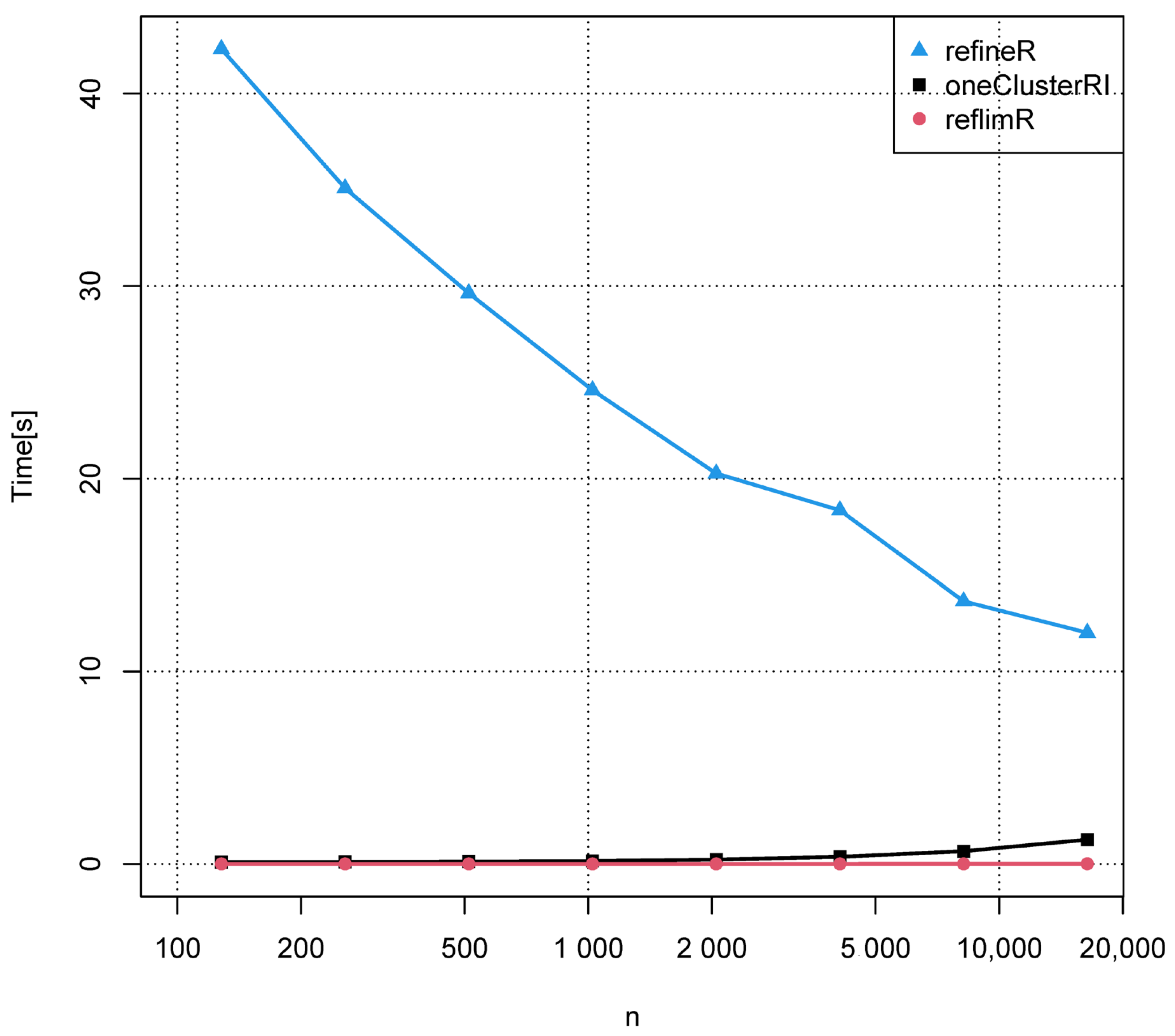
Figure 3 shows the mean computation time of the three algorithms compared in Table 1 on a standard PC. The computation time for each algorithm is computed as the mean time needed for ten artificial datasets for each sample size.

The method reflimR is the fastest one with less than one second of the computation time for all considered sample sizes, followed by oneClusterRI, also remaining below one second except for the largest sample size with a computation time of 1.3 s. The method refineR is more than a magnitude slower, especially for small sample sizes. The method refineR shows a seemingly counterintuitive behaviour concerning the computation time, which decreases with the increasing sample size. This can probably be explained by the complex statistical estimations used by refineR, leading to faster convergence for larger sample sizes that make the estimates more reliable.

6. Discussion and Conclusions

We demonstrated that it is possible to formulate an objective function with a closed-form solution for a clustering problem that avoids the otherwise computationally intensive iteration scheme. This is especially advantageous in applications where the cluster analysis itself is part of an iterative scheme as in the example of indirect reference interval estimation. The purpose of this paper was not to introduce a new method for indirect reference interval estimation but to demonstrate that a suitable formulation of the objective function for clustering can lead to a closed-form solution when the clustering problem is simplified. Of course, with the consideration of one-dimensional data with one main cluster and a noise cluster, our assumptions are very restrictive but still have an application potential as the example from laboratory medicine shows.

Our approach is of practical use whenever a dataset to be clustered consists of a main cluster with a relatively symmetric distribution and an unknown number of small clusters with unknown distributions. For example, when estimating reference intervals from “impure” values, most of which were collected from a population of healthy reference persons and a smaller proportion from persons with different diseases. While conventional methods for distribution deconvolution require statements about the distributions of the pathological fractions [33], our method allows the entirety of these sick populations to be defined as noise and the cluster of healthy individuals to be found.

Medical laboratories must evaluate their reference intervals periodically. With hundreds of analytes with different reference intervals for women, men, and various age groups, altogether thousands of reference intervals must be computed so that fast computation plays an important role. Although the different algorithms usually yield coherent reference intervals as in Table 1, in some cases one or the other algorithm fails with an implausible result. Because there is no “best” solution, it is recommended to apply different algorithms simultaneously and not to rely on a single one. With its reasonable computation time, our algorithm can therefore be seen as an additional module for computing and evaluating reference intervals.

We see another useful application in the evaluation of single-cell analyses, e.g., using flow cytometry. Here, thousands of measurement data are collected per experiment, from which the population of the cells of interest is to be recognised against the background noise of unknown other cells or particles. These can be, for example, clonal tumour cells against the background of connective tissue cells or microvesicles against the background of preparative impurities. Although flow cytometry data are in principle multidimensional, there are one-dimensional representations [38] and applications where such one-dimensional representations are the basis for the identification of the cells of interest [39].

Our results may also encourage consideration of reformulations of the objective functions in other clustering approaches, making them amenable to closed-form solutions.

The results of cluster analysis depend heavily on selecting a suitable distance measure. Here, we used the squared Euclidean distance, which, while common, is not always the best choice for all clustering problems. Replacing the Euclidean distance with a suitable other distance or dissimilarity measure might also open a path to closed-form solutions. In this way, the restrictions of our approach to one-dimensional data and one main cluster with an additional noise cluster could be overcome.

Implementations of all algorithms developed in this paper are available as R-code in the Supplementary Material.