Article

Delving into Causal Discovery in Health-Related Quality of Life Questionnaires

by
Maria Ganopoulou
1,
Efstratios Kontopoulos
2,
Konstantinos Fokianos
3,
Dimitris Koparanis
1,
Lefteris Angelis
4,
Ioannis Kotsianidis
1 and
Theodoros Moysiadis
1,*
1
Department of Hematology, University Hospital of Alexandroupolis, Democritus University of Thrace Medical School, 68100 Alexandroupolis, Greece
2
Foodpairing NV, Oktrooiplein 1 Box 401, 9000 Gent, Belgium
3
Department of Mathematics & Statistics, University of Cyprus, 1678 Nicosia, Cyprus
4
School of Informatics, Aristotle University of Thessaloniki, 54124 Thessaloniki, Greece
*
Author to whom correspondence should be addressed.
Algorithms 2024, 17(4), 138; https://doi.org/10.3390/a17040138
Submission received: 31 January 2024 / Revised: 21 March 2024 / Accepted: 22 March 2024 / Published: 27 March 2024
(This article belongs to the Special Issue Bayesian Networks and Causal Reasoning)

Abstract

:
Questionnaires on health-related quality of life (HRQoL) play a crucial role in managing patients by revealing insights into physical, psychological, lifestyle, and social factors affecting well-being. A methodological aspect that has not been adequately explored yet, and is of considerable potential, is causal discovery. This study explored causal discovery techniques within HRQoL, assessed various considerations for reliable estimation, and proposed means for interpreting outcomes. Five causal structure learning algorithms were employed to examine different aspects in structure estimation based on simulated data derived from HRQoL-related directed acyclic graphs. The performance of the algorithms was assessed based on various measures related to the differences between the true and estimated structures. Moreover, the Resource Description Framework was adopted to represent the responses to the HRQoL questionnaires and the detected cause–effect relationships among the questions, resulting in semantic knowledge graphs which are structured representations of interconnected information. It was found that the structure estimation was impacted negatively by the structure’s complexity and favorably by increasing the sample size. The performance of the algorithms over increasing sample size exhibited a similar pattern, with distinct differences being observed for small samples. This study illustrates the dynamics of causal discovery in HRQoL-related research, highlights aspects that should be addressed in estimation, and fosters the shareability and interoperability of the output based on globally established standards. Thus, it provides critical insights in this context, further promoting the critical role of HRQoL questionnaires in advancing patient-centered care and management.

1. Introduction

Health-related quality of life (HRQoL) questionnaires are standardized instruments designed to assess individuals’ perceptions of their well-being and health status. HRQoL questionnaires cover various aspects of life, including physical, psychological, emotional, and social dimensions, and they are commonly used in clinical research and healthcare to measure the impact of health conditions and treatments on individuals’ lives.
The EuroQol questionnaire with five dimensions and five levels (EQ-5D-5L) is one of the most widely used HRQoL questionnaires [1]. It was designed to assess individuals’ overall health across five dimensions: mobility, self-care, usual activities, pain/discomfort, and anxiety/depression [1]. Each dimension has five response levels, providing a more informative evaluation compared to the original EQ-5D-3L that included three response levels [2,3]. The MOS 36-Item Short-Form Health Survey (SF-36) assesses eight health domains, including physical functioning, role limitations due to physical health, body pain, general health perceptions, vitality, social functioning, role limitations due to emotional problems, and mental health [4]. The World Health Organization Quality of Life—Brief Version (WHOQOL-BREF) was developed by the World Health Organization [5] and is an abbreviated version of the WHOQOL-100 quality of life assessment [6,7,8]. It produces scores for four dimensions: physical health, psychological health, social relationships, and environment.
Health-related quality of life questionnaires specifically tailored for cancer patients aid healthcare professionals in better understanding the broader implications of cancer beyond traditional clinical measures and in tailoring supportive care strategies to enhance the overall well-being of cancer patients. Thus, they emerge as an integral tool in managing cancer patients. One of the most widely utilized HRQoL questionnaires in cancer research is the European Organization for Research and Treatment of Cancer Quality of Life Questionnaire-C30 (EORTC QLQ-C30) [9]. It assesses the HRQoL of cancer patients across physical, emotional, and social functioning domains, and symptoms such as fatigue and pain [9]. The EORTC QLQ-CLL17 is a module designed as an extension of EORTC QLQ-C30, specifically focusing on symptoms, treatment side effects, and disease-related issues unique to patients with chronic lymphocytic leukemia (CLL) [10]. By combining QLQ-C30 with QLQ-CLL17, a more enhanced understanding of the impact of CLL and its treatment on a patient’s overall well-being can be obtained. Other HRQoL questionnaires that delve into disease-specific symptoms and treatment-related concerns, thus offering a more targeted approach for specific cancer types, are included in the Functional Assessment of Cancer Therapy (FACT) measurement system [11]. The FACT system comprises a widely used set of instruments that are designed for various cancer types, such as breast cancer (FACT-B) [12], lung cancer (FACT-L) [13], colorectal cancer (FACT-C) [14], leukemia (FACT-Leu) [15], and vulvar cancer (FACT-V) [16].
There are multiple examples in the literature where HRQoL questionnaires have been employed. For example, EQ-5D-5L has been employed by the authors of [17,18,19,20], SF-36 by [21,22,23,24], WHOQOL-BREF by [25,26,27], EORTC QLQ-C30 by [28,29,30,31], QLQ-CLL17 by [31], and FACT-based questionnaires by [32,33,34,35,36]. The analysis of HRQoL data is most frequently based on descriptive statistics, standard correlation analysis, and inferential statistics (see, e.g., [37]). For instance, the correlation (Pearson, Spearman) between HRQoL scores and demographic, clinical, biological, and other parameters was assessed by the authors of [18,23,25,26,27,29,35,36]. HRQoL scores were compared either among different subgroups of patients [17,18,21,22,24,30,32] or between the subgroups of patients and controls [20,22,23,25,27,31]. Regression models have also been used to assess the correlation of HRQoL scores with various participants’ characteristics (e.g., [18,19,21,24,27,30]).
An aspect that has been so far inadequately explored in the HRQoL-related literature is causal discovery. While standard statistical correlation measures the strength and direction of a relationship between two variables, it does not necessarily imply a cause-and-effect relationship, i.e., that one of the variables is the cause of the other variable, which is considered to be the effect. Correlation does not distinguish between whether changes in one variable cause changes in another, whether both variables are influenced by a third variable, or whether the observed association is coincidental. Causal discovery goes beyond correlation analysis, aiming to infer causal relationships between variables [38]. It is a tool with wide potential that may aid to validate and/or reveal new knowledge in diverse fields (see, e.g., [39,40,41,42,43,44,45,46]). Common methods in causal discovery include causal Bayesian networks (BNs), which are graphical models representing and describing the causal relations between random variables through a directed acyclic graph (DAG), and structural equation modeling (SEM), which investigates the relationships between constructs relative to a certain phenomenon [47].
The efficient detection, assessment, and in-depth interpretation of the cause-and-effect relationships among specific HRQoL questionnaire items related to physical, psychological, lifestyle, and social parameters could offer valuable insights into patient care and management. This critical perspective motivated the current study. More specifically, understanding the causal relationships between these parameters could validate and reinforce current knowledge and/or reveal hidden aspects, thus enabling the design and implementation of more targeted strategies in patient management. For instance, if worrying about future health issues is the cause and feeling depressed is the effect, taking action to address these worries might aid to alleviate depression. A potential strategy could be to educate patients about their disease to better understand the diverse implications. Assessing the structure of the causal relationships among the questionnaire items could additionally result in understanding which are the most critical items. Namely, a specific item/node that is revealed to be the cause of several other items (thus exhibiting a high degree of centrality) stands as an important parameter to address in priority. In the previous example, if worrying about future health issues is, additionally, the cause of irritation, sleep deterioration, social alienation, etc., then it could be deducted that addressing these worries is a priority, and efforts and means should be dedicated primarily in this direction.
A few efforts have been made within the literature to examine causal relationships in HRQoL questionnaires. For instance, Krethong et al. [48] used SEM to investigate the causal relationships among bio-physiological status, social support, symptoms, functional status, general health perception, and HRQoL for Thai patients with heart failure. Structural equation modeling was also employed to examine the causal relationships between age, antiretroviral treatment, social support, symptom experience, self-care strategies, and HRQoL of people living with HIV/AIDS in the northern region of Thailand [49]. Gąsior et al. [50], on the other hand, developed a causal diagram of sport participation for children and adolescents with heart disease based on the use of an HRQoL questionnaire [51,52] by employing the Greedy Fast Causal Inference technique for continuous variables, which is a BN-based structure learning algorithm. However, the authors mentioned a limitation concerning the dataset used for identifying the DAG, since this study was based on 121 patients, which is a small sample size.
Extensive comparisons of algorithms used for causal discovery have been performed. More specifically, Scutari et al. [53] examined how different classes of causal structure learning algorithms performed in terms of the speed and accuracy of network reconstruction for both discrete BNs (involving discrete multinomial variables) and Gaussian BNs (involving continuous variables). The classes of algorithms that were assessed were constraint-based algorithms, which employ conditional independence tests, score-based algorithms, which use goodness-of-fit scores as objective functions to maximize, and hybrid algorithms, which combine the two approaches. Farnia et al. [47] similarly performed an assessment of all three classes of structure learning algorithms based on the criteria that the algorithms should be implemented by R packages, be able to analyze continuous data, and be reasonably computationally fast. To the best of our knowledge, there is no available study in the literature that focuses on the comparison of the performance of causal structural learning algorithms on discrete BNs with ordinal variables, let alone within the context of HRQoL data.
The aim in the current study was to delve into causal discovery by utilizing BNs and DAGs, specifically within the context of HRQoL questionnaire data, pinpoint the most significant considerations required for attaining reliable findings in practical HRQoL applications, and explore a comprehensive view of how to interpret the obtained results. The focus was on discrete BNs with ordinal variables, since in most cases the questions in HRQoL questionnaires require respondents to rate their perception of different aspects of their quality of life on a Likert scale. Five causal structure learning algorithms were employed on simulated data, and their performance in estimating the underlying causal structure was assessed based on diverse measures related to the complexity (number of nodes/edges) of the structure and the sample size (number of participants). The reason that we opted to use only constraint-based causal structural learning algorithms was the existence of conditional independence tests for discrete BNs with ordinal variables. Next, to elaborate further on the implications and interpretation of causal discovery results in this context, a framework is proposed for facilitating their shareability and interoperability based on the Resource Description Framework (RDF) and the relevant ecosystem of globally established standards. Efficient estimation aspects of the causal structure within the HRQoL context and the proposed interpretation perspectives have not been yet addressed in the literature, to the best of our knowledge. Exploiting these methodological tools in future HRQoL-related real-data applications could further elevate the critical role of HRQoL questionnaires in advancing patient-centered care and management.

2. Materials and Methods

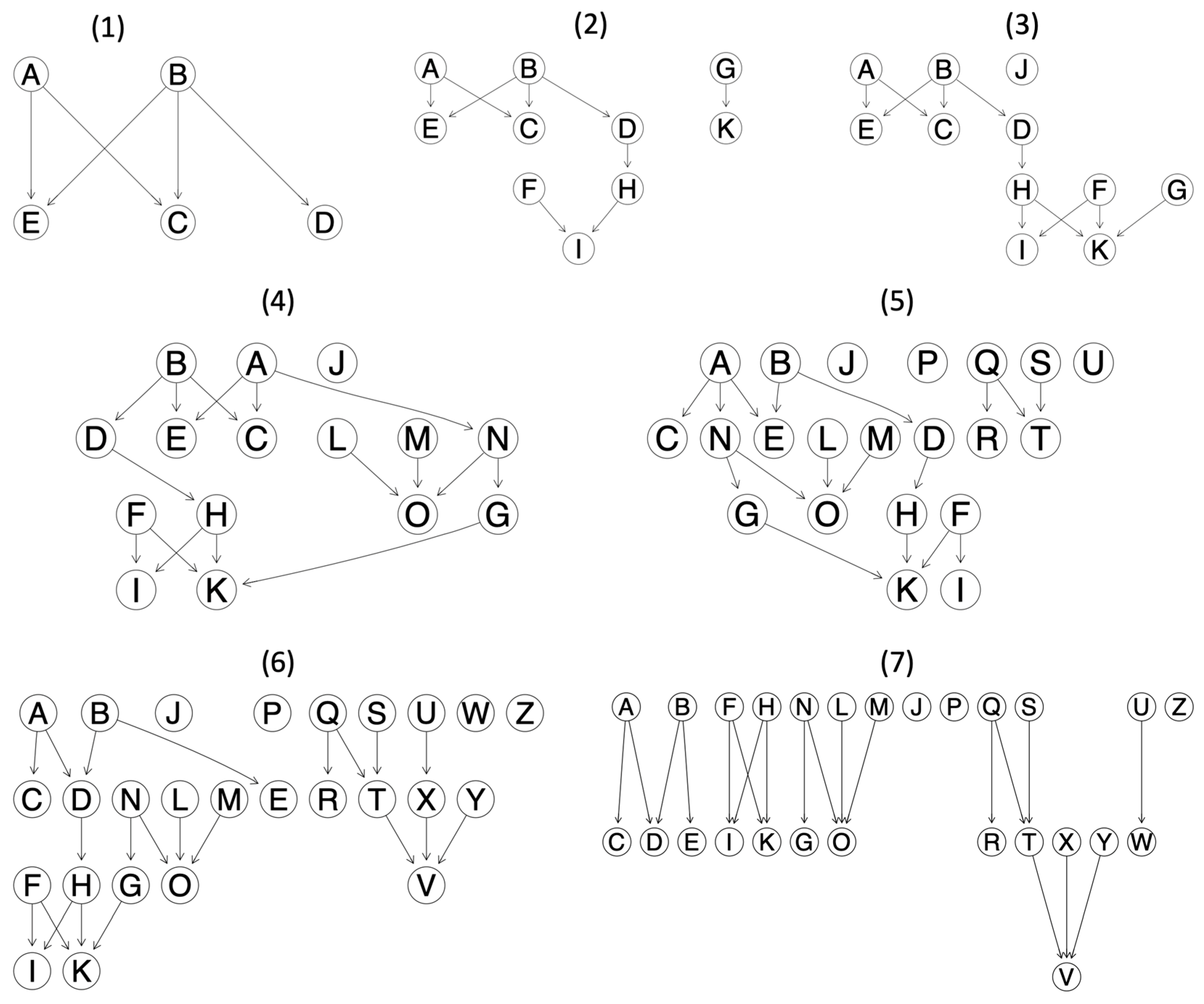
2.1. Directed Acyclic Graph

A DAG is a mathematical structure comprising nodes (also known as vertices) and directed edges (or arcs). Within the graph, there exist paths, which are sequences of adjacent edges. If an arrow connects variable X to Y, then X serves as a parent (referred to as a cause) of Y, while Y is a child (termed an effect) of X. Directed paths within the graph signify causal relationships from a starting variable to an ending variable, implying that variables act as causes for their children and effects for their parents [54]. DAGs are acyclic, namely, they lack loops or sequences of edges starting and ending at the same node. The skeleton of a DAG is the undirected graph that is formed by removing the directions of all the edges in the DAG. A v-structure is an ordered triplet of nodes (x, y, z), such that the DAG contains the edges xy and yz, and does not contain an edge between x and z. All DAGs that share the same skeleton and the same v-structures belong to the same equivalence class, called Markov equivalence class, that is represented by a completed partially directed acyclic graph (CPDAG) [55].

2.2. Methodology

2.2.1. Synthetic Directed Acyclic Graphs

The interest in this study concerns discrete BNs involving ordinal variables. Seven distinct synthetic DAGs were specified, representing the causal structures related to seven hypothetical HRQoL questionnaires (Figure 1). Both a wide range of number of questions/nodes and diverse node/edge configurations were involved, aiming to reflect the structures of causal relationships that could be encountered in real HRQoL data. Each of these HRQoL questionnaires and the corresponding DAGs involved only questions/variables that were ordinal with 4 levels. The selection of the levels was arbitrary and reflected the fact that the questions found in HRQoL questionnaires typically feature 3 to 5 answers. On the other hand, the ordered nature reflected the increasing health burden typically encountered in HRQoL questions. The aforementioned DAGs varied in the number of questions/nodes involved (ranging from 5 to 26) and the quantity of direct relationships/edges among them (ranging from 5 to 19).
The tailored parameter specifications for each DAG were defined using the R package “bnlearn” [56] (Version 4.9) and can be found at a dedicated GitHub repository (https://github.com/teomoi/Causal-HRQoL) that has been developed for this study. The seven synthetic DAGs have not been used before in the literature in any causal-discovery-related or other context.

2.2.2. Simulations

The seven synthetic DAGs were then used to generate simulated data using the R package “bnlearn” [56]. In particular, the “rbn” function was used to simulate random samples from each DAG. The sample size, namely the number of simulated participants (completed questionnaires), was denoted by n. For each DAG and for different values of n (100, 500, 1000, 2000, 5000, 10,000), 1000 samples were generated. Next, for each DAG, each simulated sample of size n was used to estimate the underlying causal structure and, in particular, its equivalence class, represented by a CPDAG, by employing five constraint-based causal structural learning algorithms that used conditional independence tests to learn the dependence structure of the data. All five algorithms were implemented with the R package “bnlearn” [56].
In particular, the constraint-based algorithms were as follows:
  • PC [57], employing the “pc.stable” function: A modern implementation of the PC algorithm, the first practical constraint-based structure learning algorithm, with PC standing for Peter Spirtes and Clark Glymour [58,59].
  • Grow–Shrink (GS) [60], employing the “gs” function: This is based on the Grow–Shrink Markov blanket, which is a Markov blanket detection algorithm.
  • Incremental Association (IA) [61], employing the “iamb” function: This is based on the Markov blanket detection algorithm of the same name.
  • Interleaved Incremental Association (Inter-IA) [62], employing the “inter.iamb” function: This is a variant of the IA algorithm, which differentiates in using gradual forward selection to avoid false positives in the Markov blanket detection phase.
  • Fast Incremental Association (Fast-IA), employing the “fast.iamb” function: This is another variant of the IA algorithm that employs speculative stepwise forward selection to reduce the number of conditional independence tests.
For all the above algorithms, the default arguments were employed. The conditional independence test that was used by default for ordered factors within the “bnlearn” R package was the Jonckheere–Terpstra test.
The performance of the algorithms regarding accuracy in structural reconstruction was assessed with measures related to (i) the Hamming distance (HD), which computes the differences between the skeletons of two DAGs, and (ii) the structural Hamming distance (SHD), which is based on the comparison between the corresponding CPDAGs of two DAGs [63]. In particular, SHD accounts for the number of operations required to make two CPDAGs match, or more specifically, to add or delete an undirected edge, and add, remove, or reverse the orientation of an edge. The computation of HD and SHD was performed with the R functions “hamming” [56] and “shd” [56], respectively. More specifically, for each DAG and each n , represented by the corresponding 1000 iterations, and for each algorithm, the following measures were used to compare the estimated and the underlying/true causal structures:
  • The mean HD between the estimated and the true DAG across the 1000 iterations.
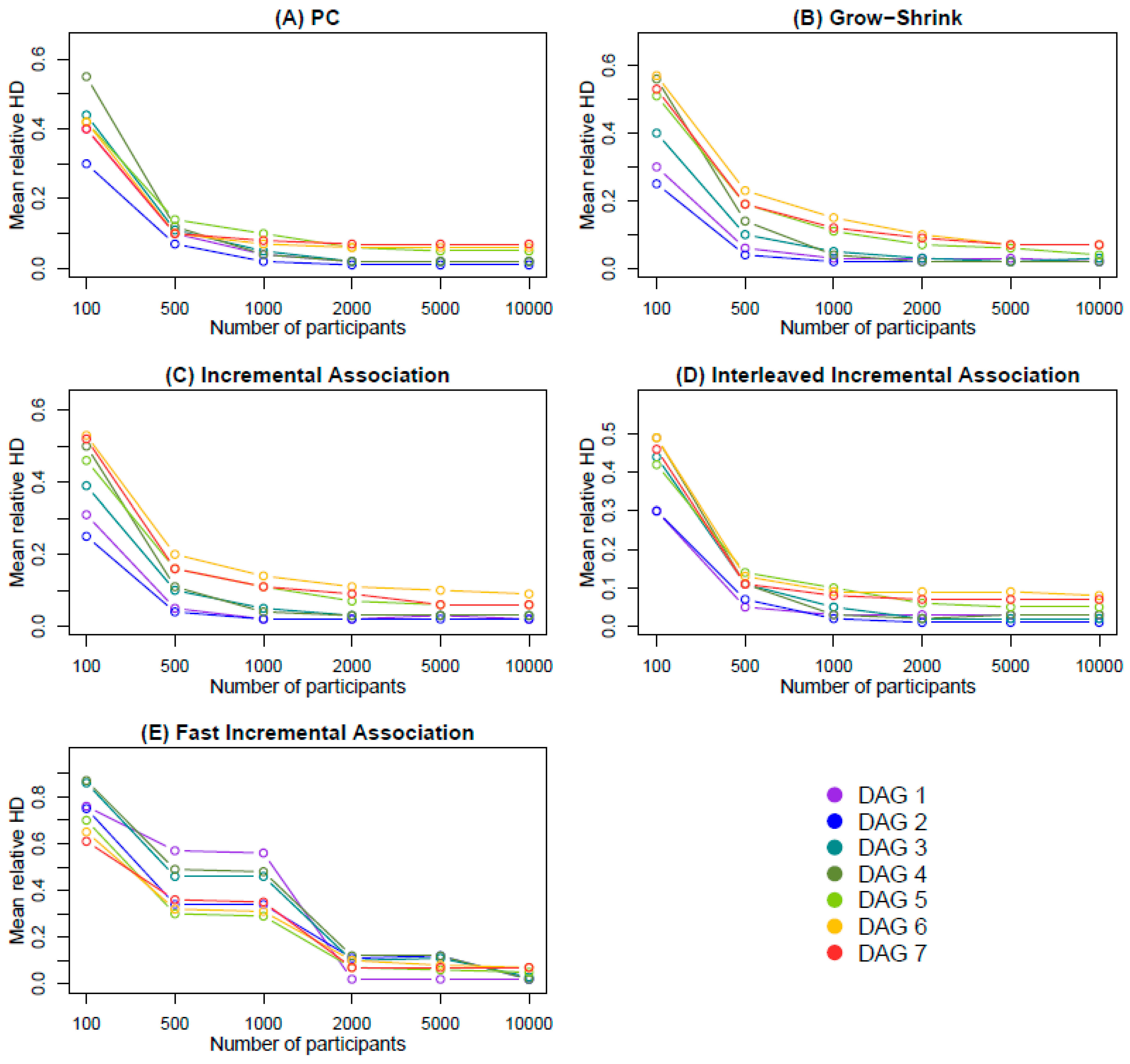
  • The mean relative HD across the 1000 iterations, defined as the mean HD between the estimated and the true DAG, divided by the number of edges of the true DAG.
  • The number of the cases where the HD between the estimated and the true DAG was zero across the 1000 iterations.
  • The mean SHD between the estimated and the true DAG across the 1000 iterations.
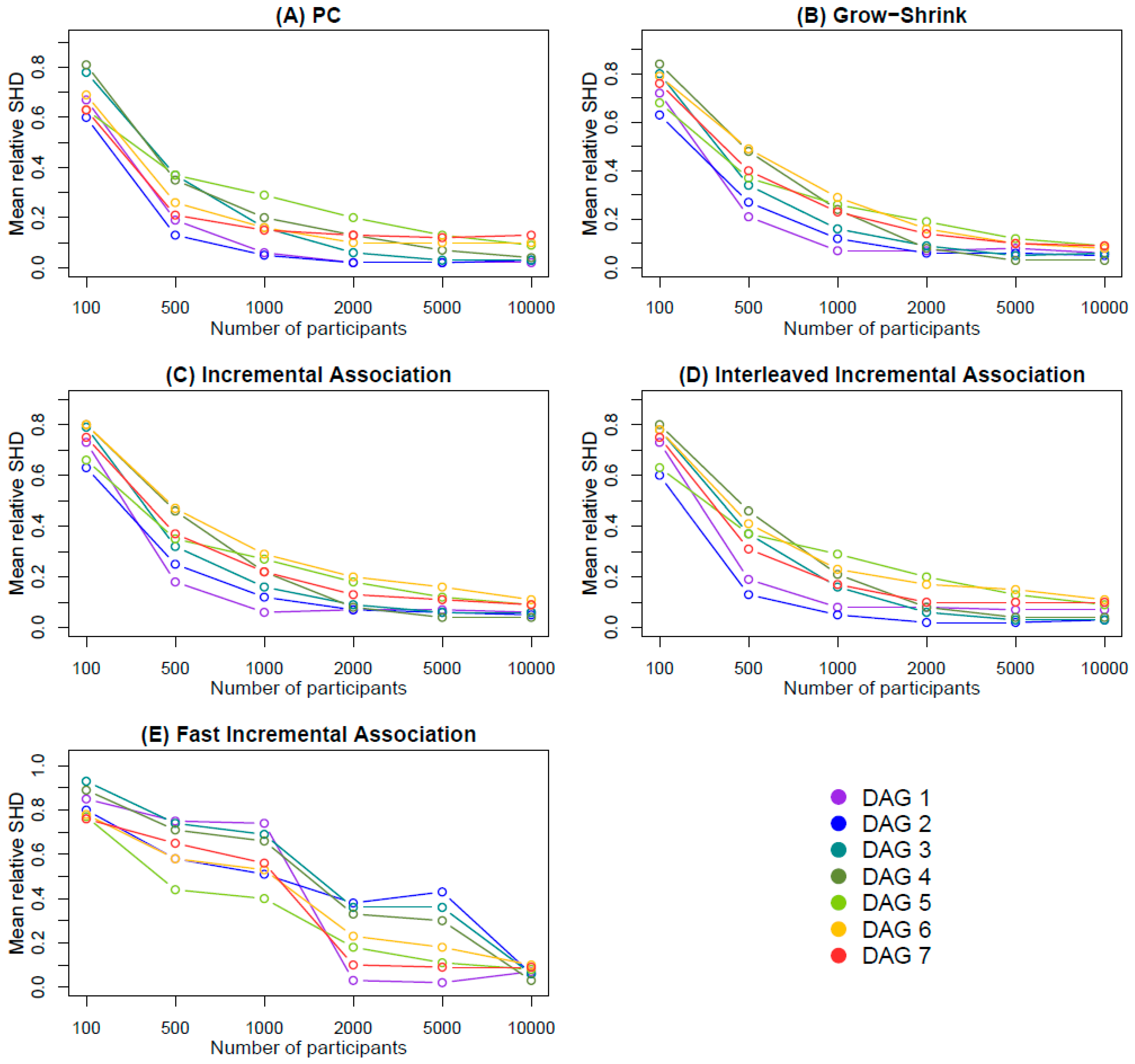
  • The mean relative SHD across the 1000 iterations, defined as the mean SHD between the estimated and the true DAG, divided by the number of edges of the true DAG.
  • The number of cases where the SHD between the estimated and the true DAG was zero across the 1000 iterations.
The two relative measures were used in order to account for the differences in network size and complexity, and assumed values between 0 and 1. All analyses were performed with R, v.4.2.1. The R code used for the simulations is available at (https://github.com/teomoi/Causal-HRQoL).

2.2.3. Shareability and Interoperability

In order to facilitate the shareability and interoperability of our findings, we adopted the Resource Description Framework [64] to represent the responses to the HRQoL questionnaires, as well as the cause–effect relationships among the questions. The RDF constitutes a core technology in the ecosystem of semantic technologies endorsed by the World Wide Web Consortium (W3C) and serves as the backbone for creating semantic knowledge graphs (KGs). Semantic KGs are structured representations of interconnected information and enhance understanding and retrieval for both humans and machines [65].
In essence, a semantic KG assumes the form of a directed graph, where the nodes represent the various entities of the domain of interest and the edges represent their interrelationships. The graph becomes “semantic” when the meanings (i.e., semantics) of every node and edge are explicitly specified in a human- and machine-understandable format like the RDF. This way, the KG constitutes a model of the domain at hand that can be easily shared/exchanged, but also effortlessly processed by programs and automated (intelligent) tools, like AI agents.
Specifically, for the representation of HRQoL questionnaires as RDF KGs, as well as the involved questions, the patients’ responses, and the cause–effect relationships between questions, we relied on DDI-RDF [66], a vocabulary for publishing metadata about datasets (research and survey data). Moreover, in HRQoL questionnaires, every question typically corresponds to a facet, and each facet can be further categorized in a domain (e.g., physical, psychological, emotional, social, etc.). In our approach, we represented facets and domains as SKOS concepts, where SKOS (Simple Knowledge Organization System) is a W3C standard for representing knowledge organization systems [67]. Additionally, SKOS also allows the representation of narrower–broader relationships between concepts, and this facilitated the representation of the associations between facets and domains, resulting, in essence, in a two-level taxonomy. All KGs discussed in this work are serialized in RDF Turtle, which represents knowledge as <subject-predicate-object> triples.
Our motivation behind this whole endeavor was twofold: (a) to facilitate collaboration with potentially interested third parties towards developing extensions of mutual interest across research studies and healthcare institutions, and (b) to drive knowledge discovery from HRQoL data towards developing decision support systems that leverage semantic technologies in the context of patient management.

2.2.4. Available Resources

To facilitate the reproducibility of the methodology, detailed documentation is provided at https://github.com/teomoi/Causal-HRQoL, a repository that has been developed specifically for this study. In particular, the R script “2024 Causal Discovery-HRQoL-7 DAGs_github.R” refers to Section 2.2.1 and the development of the seven synthetic DAGs. The R script “2024 Causal Discovery-HRQoL-Simulation_github.R” refers to Section 2.2.2 and includes the customized function that was used for random sample simulation, causal structure estimation using the five constraint-based causal structural learning algorithms, an assessment of the algorithms’ performance, and a specific usage example. The GitHub repository also contains the schema (i.e., the “ontology”) of the KG discussed in this work, along with supplementary descriptions.

3. Results

3.1. Simulation Findings

The analytical results of all the assessment measures considered for causal structure estimation based on the PC, the Grow–Shrink, the Incremental Association, the Interleaved Incremental Association and the Fast Incremental Association algorithms are available in Appendix A (Table A1, Table A2, Table A3, Table A4 and Table A5, respectively).
By assessing Table A1, Table A2, Table A3, Table A4 and Table A5, it was observed that the mean values corresponding to the Hamming distance and the structural Hamming distance increased in most cases as the structure complexity increased, and decreased as the sample size increased. For example, in Table A2 (GS algorithm), at n = 100 , the HD increased from 1.48 to 11.89 as the complexity of the DAGs increased, at n = 500 , it increased from 0.31 to 4.83, at n = 1000 , the HD increased from 0.14 to 3.07 as the DAGs’ complexity increased, and similarly at n = 2000 , the HD increased from 0.13 to 2.16. At n = 5000 , it increased from 0.15 to 1.55, and at n = 10,000 , the HD increased from 0.11 to 1.37. It is easy to observe that the HD values were larger for smaller values of n , while they gradually decreased as n increased. This behavior was observed in almost all cases, but it was less pronounced in the case of the Fast-IA algorithm (Table A5).
At the same time, the values corresponding to the HD were, in general, lower than the ones corresponding to the SHD. In the same example of the GS algorithm, it is shown in Table A2 that, at n = 100 , the SHD increased from 3.60 to 16.65 as the complexity of the DAGs increased, at n = 500 , it increased from 1.03 to 10.37, at n = 1000 , it increased from 0.37 to 6.16 as the DAGs’ complexity increased, at n = 2000 , the SHD increased from 0.35 to 3.26, at n = 5000 , it increased from 0.41 to 2.13, and at n = 10,000 , the SHD increased from 0.29 to 1.76. Similarly, as in the case of the HD, the SHD values were larger for smaller values of n , and they decreased as n increased. In the case of the Fast-IA algorithm (Table A5), it was observed that the less complex DAGs #1, 2, 3, and 4 exhibited, for some values of the sample size n , comparable or even higher SHD values, compared to the more complex DAGs #5, 6, and 7 (see, e.g., n = 2000 ,   5000 in Table A5).
The assessment results regarding the mean relative HD and the mean relative SHD are visually displayed in Figure 2 and Figure 3, respectively. In particular, by assessing the mean relative HD (Figure 2), it is shown that the PC (Figure 2A) and the Inter-IA (Figure 2D) algorithms exhibited the best performance, since both of them demonstrated a mean relative HD less than or equal to 0.15 for all DAGs, even at n = 500 , and less than or equal to 0.10 for all DAGs at n = 1000 or higher. The PC algorithm exhibited slightly lower values compared to the Inter-IA algorithm for large sample sizes ( n = 2000 ,   5000 ,   10,000 ). The GS (Figure 2B) and IA (Figure 2C) algorithms both required the sample size to be at least 1000 in order for the mean relative HD to be less than or equal to 0.15 for all DAGs, and it was less than or equal to 0.10 for all DAGs at n = 2000 or higher (with the exception of the IA algorithm, DAG #6, at n = 2000 ). The Fast-IA (Figure 2E) was the only algorithm that required at least n = 2000 in order for the mean relative HD to be less than or equal to 0.15 for all DAGs.
By assessing the mean relative SHD (Figure 3), it was observed that the algorithms PC, GS, IA, and Inter-IA (Figure 3A–D) exhibited similar behavior across all values of n with a mean relative SHD being less than or equal to 0.30 for all DAGs at n = 1000 , less than or equal to 0.20 for all DAGs at n = 2000 , and less than or equal to 0.15 for all DAGs at n = 10,000 . The Fast-IA algorithm (Figure 3E) exhibited large values of mean relative SHD even for n = 5000 .
The number for successfully estimating the whole causal structure across the 1000 iterations, represented by the number of zero values in either the HD or the SHD, was observed to be higher for simpler structures and increased as the number of participants n increased. For instance, in the case of the PC algorithm (Table A1), even at n = 500 , for the simpler DAGs #1 and 2, the number of zero values in HD across 1000 iterations was 532 and 491, respectively, while for the more complex DAGs #5, 6, and 7, the corresponding numbers were 45, 84, and 142, respectively (Table A1). At n = 10,000 , DAGs #1 and 2 exhibited 905 and 885, respectively, as the number of zero values in HD across 1000 iterations, while DAGs #5, 6 and 7 exhibited 445, 249, and 232, respectively. The numbers of zero values in the SHD case were in general lower than the corresponding ones in the HD case. In the previous example, it is shown in Table A1 that at n = 500 , for the simpler DAGs #1 and 2, the numbers of zero values in SHD across 1000 iterations were 526 and 479, respectively, while for the more complex DAGs #5, 6, and 7, the corresponding numbers were 8, 20, and 48, respectively. At n = 10,000 , however, the values were almost identical with the HD case, with DAGs #1 and 2 exhibiting 905 and 885, respectively, and DAGs #5, 6, and 7 exhibiting 390, 249, and 232, respectively. Similar results apply for all the algorithms.
Additionally, it was observed that the difference in zero values among the least complex and most complex DAGs was in most cases very large. For example, when assessing the SHD considering the Inter-IA algorithm, at n = 500 , DAGs #1 and 2 exhibited 737 and 479 for the number of zeros in SHD across 1000 iterations, while for DAGs #5, 6, and 7, the corresponding numbers were 8, 0, and 6, respectively (Table A4). At n = 1000 , DAGs #1 and 2 exhibited 871 and 797, respectively, while the number of zeros in SHD in DAGs #5, 6, and 7 was 46, 22, and 85, respectively. Finally, at n = 10,000 , DAGs #1 and 2 exhibited 864 and 885, respectively, while the number of zeros in SHD in DAGs #5, 6, and 7 was 390, 177, and 238, respectively. This level of difference was observed across all algorithms for both HD and SHD.
In addition, more complex structures, such as DAGs #5, 6, and 7, exhibited higher values of relative HD/SHD compared to less complex structures such as DAGs #1, 2, and 3, or even #4. This was particularly evident in the case of the relative HD (Figure 2), in which the values corresponding to DAGs #5, 6, and 7 were in almost all cases higher than those corresponding to the remaining DAGs for all algorithms apart from the Fast-IA algorithm. In particular, at n = 1000 or higher, a clear distinction is observed at the level of the values corresponding to the group of DAGs #5, 6, and 7 and the group of DAGs #1, 2, 3, and 4. For instance, in the case of the GS algorithm (Figure 2B, Table A2), at n = 1000 , the relative HD values for DAGs #1, 2, 3, and 4 were 0.03, 0.03, 0.05, and 0.04, while for DAGs #5, 6, and 7 the corresponding values were much higher (0.11, 0.15, and 0.12). At   n = 2000 , the relative HD values for DAGs #1, 2, 3, and 4 were 0.03, 0.02, 0.03, and 0.02, while for DAGs #5, 6, and 7 the corresponding values were 0.07, 0.10, and 0.09. Even at   n = 10,000 , the values’ level differences between these two groups were still observed, since the relative HD values for DAGs #1, 2, 3, and 4 were 0.02, 0.02, 0.03, and 0.02, while for DAGs #5, 6, and 7 the corresponding values were 0.04, 0.07, and 0.07. Similar differences in the relative HD values between the groups of DAGs #1, 2, 3, and 4 and DAGs #5, 6, and 7 were observed in the case of the PC, IA, and Inter-IA algorithms (Figure 2A,C,D).
In the case of the relative SHD (Figure 3), the difference between the groups of more complex and less complex DAGs was less pronounced. Still, the values corresponding to DAGs #5, 6, and 7 were in general higher than those corresponding to the remaining DAGs for all algorithms apart from the Fast-IA algorithm. However, this distinction was more evident for higher values of sample size compared to the case of relative HD, in particular, at n = 2000 or higher. Assessing, for instance, the case of the GS algorithm (Figure 3B, Table A2), at n = 1000 , the relative SHD values for DAGs #1, 2, 3, and 4 were 0.07, 0.12, 0.16, and 0.24, while for DAGs #5, 6, and 7 the corresponding values were 0.26, 0.29, and 0.23, i.e., in the case of DAG #4, the value is comparable to DAGs #5, 6, and 7. At   n = 2000 , the relative SHD values for DAGs #1, 2, 3, and 4 were 0.07, 0.06, 0.09, and 0.08, while for DAGs #5, 6, and 7 the corresponding values were 0.19, 0.16, and 0.14. At   n = 10,000 , the relative SHD values for DAGs #1, 2, 3, and 4 were 0.06, 0.05, 0.06, and 0.03, while for DAGs #5, 6, and 7 the corresponding values were 0.09, 0.08, and 0.09.
On the other hand, despite the differences between algorithms, the pattern evolution of the measures’ values over the sample size was similar in each algorithm. Namely, the performance of each algorithm based on the HD, the SHD, and the number for successfully estimating the whole causal structure across the 1000 iterations improved in a similar manner with increasing sample size for all the seven structures considered (see, e.g., Figure 2 and Figure 3A–D). The only exception was the Fast-IA algorithm in the case of the mean relative SHD (Figure 3E). In addition, the algorithms PC, GS, IA, and Inter-IA exhibited a similar pattern evolution among each other as well, both in the case of HD (Figure 2A–D) and in the case of SHD (Figure 3A–D).

3.2. Resource Description Framework Knowledge Graph

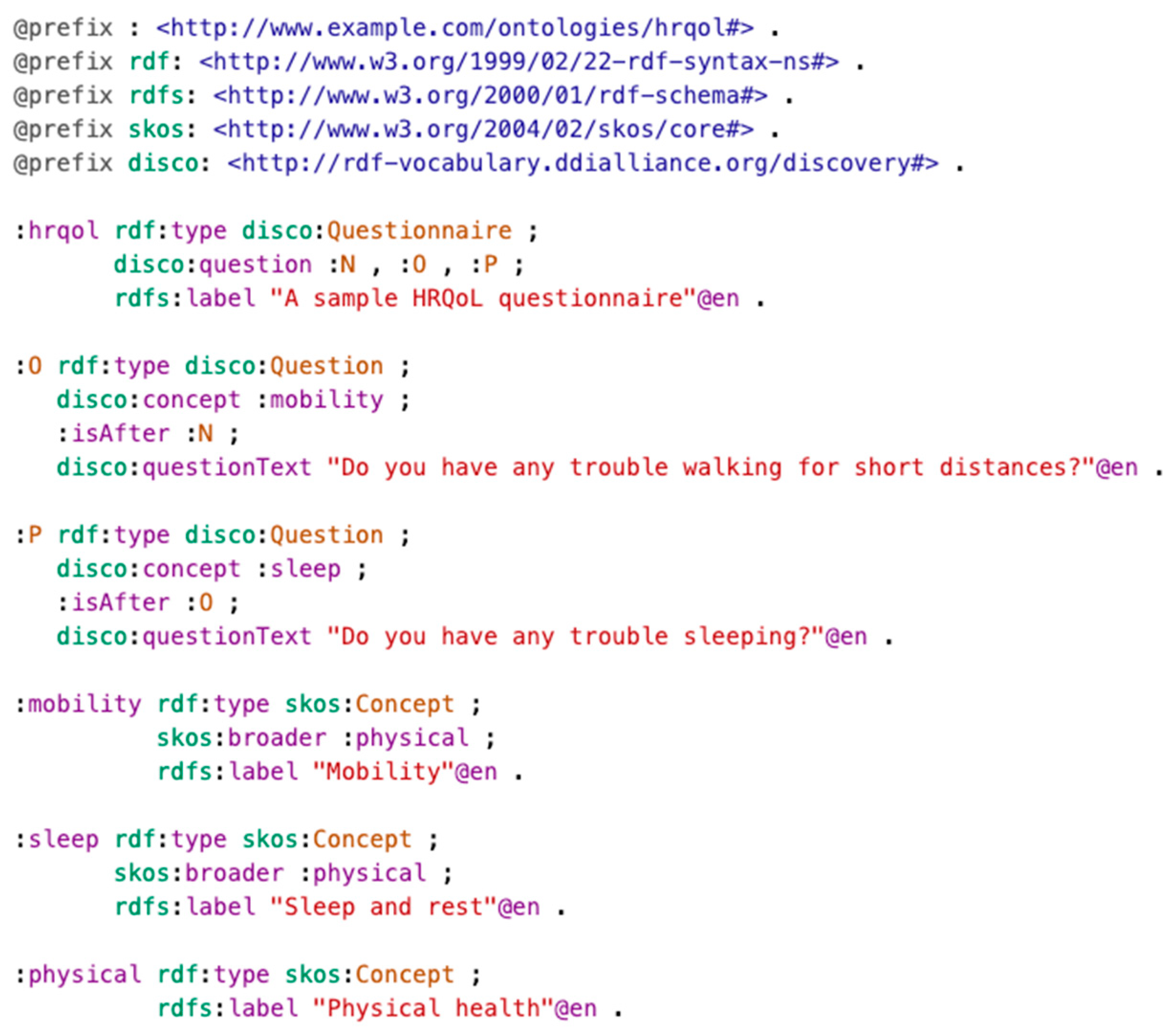
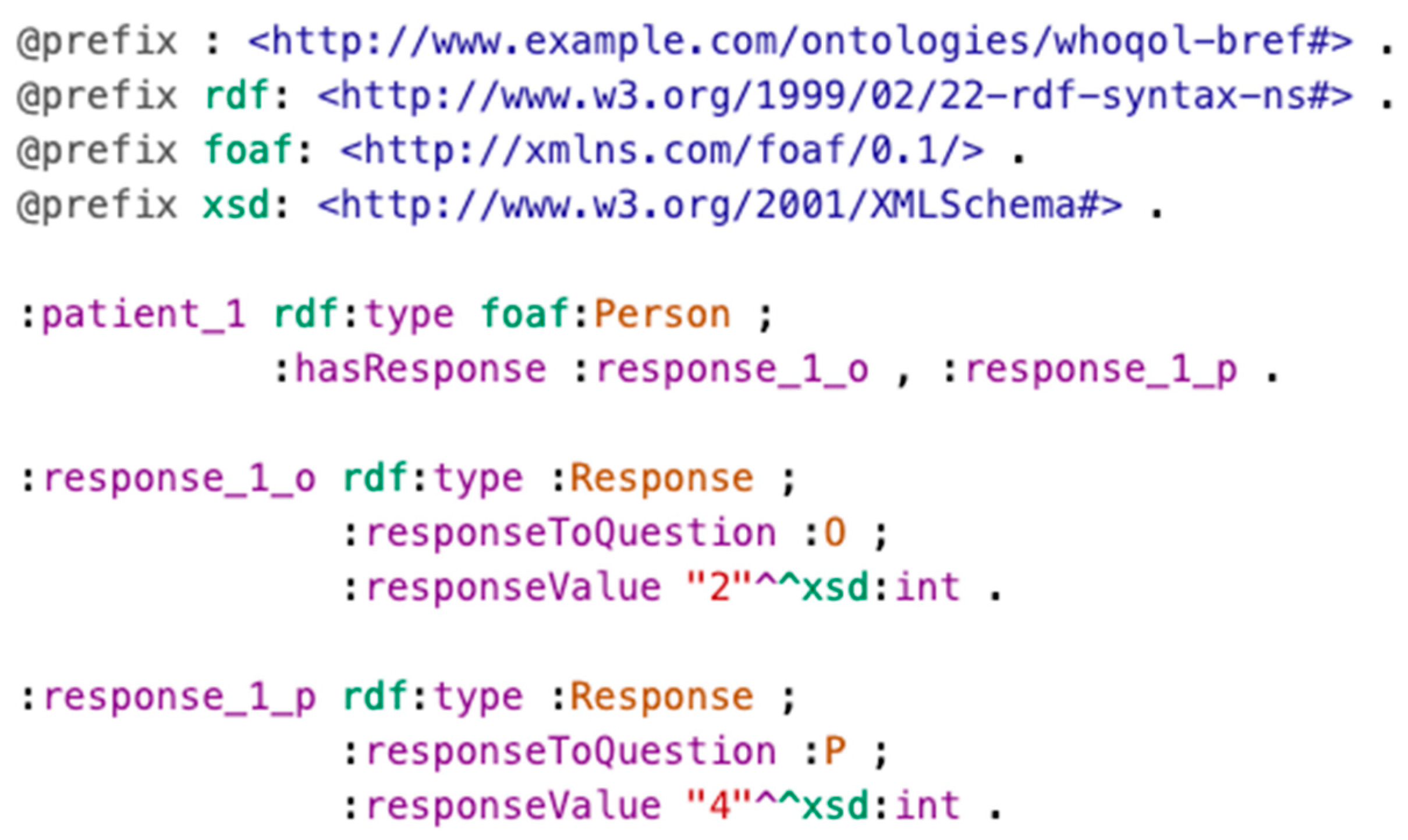
3.2.1. Representing Questionnaires and Responses

A hypothetical HRQoL questionnaire corresponding to DAG #6 (Figure 1(6)) was used as an example, and was represented according to the proposed methodology as a semantic model (i.e., as an RDF KG) based on DDI-RDF. Figure 4 illustrates a representation of a fragment of this hypothetical questionnaire in RDF Turtle serialization.
The namespace prefixes at the top of the Turtle excerpt correspond to existing semantic models available on the Web; the “disco” prefix corresponds to DDI-RDF, while prefix “:” refers to the base prefix corresponding to a fictional namespace devised for the purposes of this example.
With regard to the structure of the KG, we note the following points:
The excerpt shown in the figure only includes three sample hypothetical questions for illustration purposes. The representation of an actual HRQoL questionnaire would include all the questions.
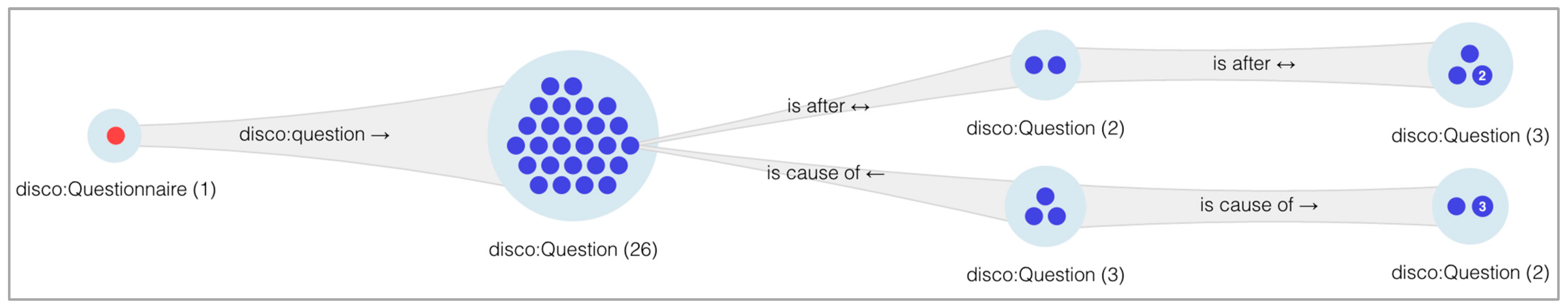
In order to also represent the order of questions in the questionnaire, every question contains information about the previous one via predicate “:isAfter”.
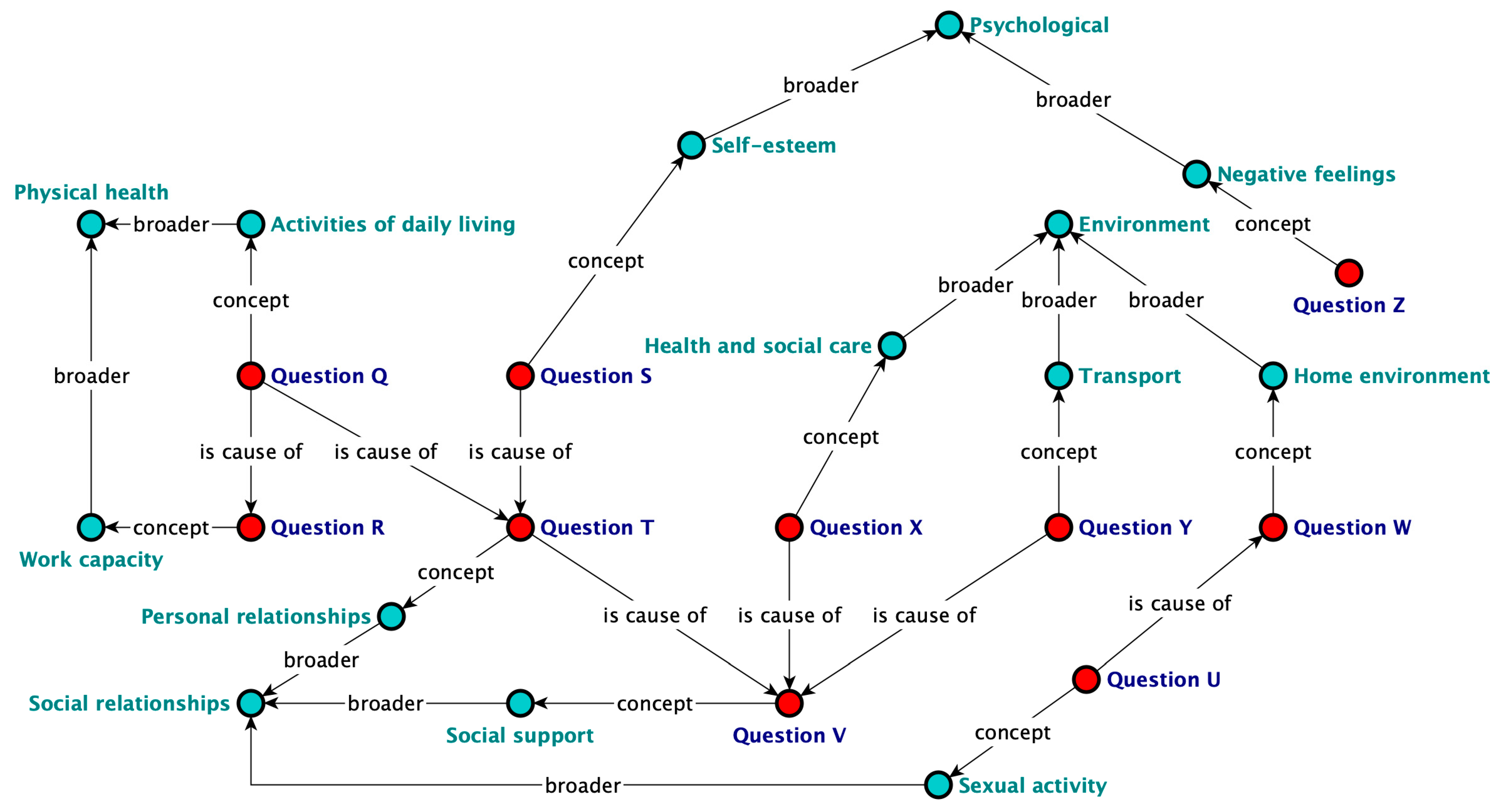
The association of questions to facets (see Section 2.2.3) is materialized via DDI-RDF predicate “disco:concept”.
The association of facets to domains is materialized via SKOS predicate “skos:broader”, which represents a narrower–broader interrelationship.
In a similar fashion, the patients’ responses were serialized in RDF Turtle, as seen in Figure 5.
The excerpt represents a sample hypothetical patient and their responses to questions “O” and “P”, which are specified in Figure 4. In this case, the responses assume integer values ranging from 1 to 4.

3.2.2. Representing Cause–Effect Relationships

Still remaining within the RDF realm, the cause–effect relationships among the questions were also represented in the same manner. Figure 6 illustrates a subset from synthetic DAG #6 (see Figure 1(6)) where the cause–effect relationship between questions (red nodes) was represented via the property “isCauseOf”. The order of questions in the questionnaire via the predicate “:isAfter” was not displayed in Figure 6, since in this example it was trivial and corresponded to the alphabetical order of the questions (e.g., T is after S). Figure 6 also includes hypothetical facets corresponding to each question along with respective hypothetical second-level domains (both facets and domains are illustrated as cyan nodes). For instance, question Q is the cause of question R. Moreover, question Q has a facet of “Activities of daily living”, question R has a facet of “Work capacity”, and both of the facets belong to the same second-level domain “Physical health”.
Next, Table 1 indicates the respective intensities of the inter-domain associations based on sample DAG #6. Associations of a specific domain to itself were not taken into account. For instance, “Environment” was observed to be the cause domain of “Physical Health” three times; namely, a cause–effect relationship with the cause variable belonging to the domain of “Environment” and the effect variable belonging to the domain of “Physical Health” was observed three times in total. On the other hand, a cause–effect relationship with the cause variable belonging to the domain of “Social relationships” and the effect variable belonging to the domain of “Environment” was observed only once.

4. Discussion

4.1. Causal Discovery

In order to achieve reliable results in a real-data HRQoL application, several aspects should be taken into account. The simulation results in this study indicated that the performance of different constraint-based algorithms was influenced by both the complexity of the underlying causal structures and the sample size. Overall, the mean values corresponding to both the HD and the SHD (and the corresponding relative measures) generally increased as the number of nodes/edges increased, and decreased as the sample size increased, with the HD values being lower, in general, compared to the corresponding SHD values. Similarly, the number of zero values in both HD and SHD across the 1000 iterations was observed to be lower for more complex structures and increased as the sample size increased, with the numbers of zero values in the SHD case being in most cases lower than the corresponding ones in the HD case. The pattern evolution of the measures’ values over the sample size was similar in each algorithm across all DAGs considered. In addition, the algorithms PC, GS, IA, and Inter-IA exhibited a similar pattern evolution among each other in the cases of both HD and SHD.
In the more complex DAGs #5, 6, and 7, which demonstrated a range of 21–26 in the number of nodes and 17–21 in the number of edges, compared to the simpler DAGs #1, 2, 3, and 4, which demonstrated a range of 5–25 in the number of nodes and 5–16 in the number of edges, higher mean values were exhibited in both HD and SHD in almost all cases, and for all algorithms, excluding the Fast-IA algorithm. Similarly, by assessing the number of successful estimations of the whole causal structure across the 1000 iterations, the algorithms exhibited the best performance in the simpler DAGs #1 and 2, and the worst in the more complex DAGs #5, 6, and 7. On the other hand, by increasing the sample size, the performance of the algorithms, considering all measures of assessment, improved and usually started to converge for values of n equal to or higher than 2000.
These results were expected to some extent, since, intuitively, a more complex underlying causal structure is harder to estimate in an efficient manner compared to a less complex structure, while a larger sample size is connected, in general, to more robust estimation. A similar result regarding the performance improvement when the sample size is larger was observed by Farnia et al. [47], although in that study the impact of the sample size was assessed for continuous variables in the presence/absence of latent confounders. Regarding the complexity of the structure/network, Scutari et al. [53] concluded that by comparing small networks (less than 50 nodes) versus large networks (more than 50 nodes), no systematic differences in the accuracy of network reconstruction were observed in the rankings of the learning algorithms that were assessed. Although this seems to be contradictory to the results in our study, it should be noted that networks of similar size may demonstrate large differences in the number of parameters and thus large differences in their levels of complexity, as is stated as well by Scutari et al. [53]. Therefore, the distinction based on the number of nodes does not represent an explicit distinction in structure complexity. On the other hand, in our study, the complexity of the structure is reflected in both the number of nodes and edges. In addition, in the simulation study [53], a concept of relative sample size was employed (n/|Θ|), accounting for the number of network parameters (|Θ|). To sustain the same relative sample size, larger values of absolute sample size ( n ) were required for more complex networks. Thus, although the structure learning algorithms did not exhibit differences in their accuracy rankings between small and large networks, the comparison was based, in general, on larger absolute sample size values for more complex networks compared to less complex networks. Thus, these results are in accordance with our results, since the values of the measures considered were comparable between more complex networks for larger absolute sample size and less complex networks for smaller absolute sample size.
The observation that the HD values were, in general, lower than the corresponding SHD values is mainly attributed to the fact that HD only accounts for differences in the skeletons of DAGs, while SHD refers to the direction of the relationships as well.
On the other hand, the similarities in the pattern evolution of the assessment measures’ values over the sample size across the seven different structures in each algorithm indicate that the structure complexity did not constrain the improvement of the algorithms’ performance as the sample size increased. On the contrary, the improvement pattern was observed to be independent of the complexity and mainly dependent on the sample size at hand. The only exception was the Fast-IA algorithm, which, particularly in the case of SHD, demonstrated different evolution patterns across the seven DAGs (Figure 3E). It should be noted, however, that despite the fact that the algorithms exhibited, in general, similar pattern evolutions regarding both HD and SHD and all algorithms performed quite well for large sample sizes, they exhibited noticeable differences for small sample sizes, more specifically at n = 500 . It is shown in Figure 2 that the PC and the Inter-IA algorithms exhibited clearly lower mean relative HD values at n = 500 compared to all the remaining algorithms. This behavior was observed as well in the case of SHD (Figure 3). In addition, the level of complexity of the initial structure had an impact on the value level of relative HD and relative SHD; namely, in more complex structures such as DAGs #5, 6, and 7, the observed values were higher compared to less complex structures.

4.2. Knowledge Representation via Semantic KGs

By representing the derived outcomes from this work as a KG that complies with globally established W3C standards, three important aspects were facilitated: (a) shareability, by allowing potentially interested third parties to easily adopt our work and possibly extend it, (b) collaboration, by laying the groundwork for forming a community of stakeholders with shared interests that “speak the same language” with the proposed RDF-KG, and (c) interoperability with third-party applications and AI agents that may capitalize on our outputs to reach their own research goals.
Additionally, by representing this work using semantic technologies, its impact is elevated by providing a framework that makes the data actionable, namely, facilitating the extraction of insights that can be readily used to make informed decisions. For instance, Figure 6 showcases, on top of the cause–effect relationships, the facets corresponding to each question, along with the corresponding second-level domains. Having the latter in the KG allows for a degree of deeper semantic analysis of the DAG. For instance, a cause–effect relationship can be additionally explained based on the facets and/or broader domains that correspond to the questions involved. Moreover, the total number of cause–effect associations between domains can be easily retrieved, providing an additional layer of interpretation. For the example of DAG #6 (Figure 1(6)), Table 1 summarizes the total count of the inter-domain associations. By obtaining this information in a real-data application, it can be inferred which broad domains are strongly connected to each other and in which direction, at the specific instance that the questionnaires were completed by the participating individuals. In this specific hypothetical example, the environment seems to have a strong effect on the physical health, psychological, and social relationships domains. It should be noted that, in general, not all questions in an HRQoL questionnaire have a facet and/or a second-level domain, and relevant interpretations are strongly related to the HRQoL questionnaire choice.
Despite its increased utility in data representation, the RDF is arguably challenging to work with, especially for non-specialists who could benefit from a user-friendly approach that would enhance accessibility and understanding while visualizing and traversing the KG. Fortunately, several software tools exist that address those needs and capitalize on the graph representation intrinsic to the RDF model [68]. Some representative examples include OntoGraf, a visualization plugin contained in the popular KG management tool Protégé v5.6.3 [69], as well as SemSpect, a flexible tool that deploys visual aggregation to solve the “hairball problem” looming in visualizing large graphs [70]. Figure 7 illustrates the use of the latter tool for visualizing a sample KG; users can freely move in both directions of the cause–effect relationships between responses to questions in an HRQoL questionnaire.
Through user-friendly visual representations like the ones discussed above, users can intuitively navigate and interact with the KG in a “follow your nose” fashion, leveraging features like zooming, filtering, and interactive exploration. As a result, the integration of visualization methods fosters greater engagement and participation from diverse stakeholders.

4.3. Impact, Limitations, and Future Work

Overall, the purpose of this study was to highlight the dynamics of applying causal discovery using BNs and DAGs specifically within the HRQoL context, the most important aspects that should be taken into account in a real HRQoL application in order to reach reliable results, and the wide possibilities of results’ interpretations. The selected causal structure learning algorithms were assessed under different specifications of sample size, number of nodes, number of edges, and, in general, network structure. The results in this study could be used as a guide for researchers opting to employ causal discovery in a real-data application involving HRQoL data. Namely, this study could aid the choice/design of HRQoL questionnaires (number of items involved), appropriately setting the sample size by exploiting scientific intuition regarding the underlying causal structure, and assessing different algorithm options. An additional layer for when sample size limitations exist, which is often the case in real-data applications, could be to perform a preliminary assessment. More specifically, a preliminary analysis could be employed in order to estimate the performance of an algorithm under a specific HRQoL questionnaire (number of items), the prior knowledge regarding its underlying causal structure, and the existent limitations concerning the number of participants that could be included in the study. Globally established W3C-endorsed semantic technologies can be employed to further enrich the results of causal discovery and to provide the basis for deeper interpretations. To facilitate the interested user to apply the methods covered in this study, a dedicated GitHub repository has been developed, including detailed documentation (https://github.com/teomoi/Causal-HRQoL).
Causal discovery within the HRQoL questionnaire context is a highly promising tool. Efficient estimation of the causal structure among HRQoL items and the elaborate interpretation of the obtained results could boost the vital role of HRQoL questionnaires in better understanding the different aspects of an individual patient’s well-being and promoting patient-centered care and management.
A limitation of the study is that the algorithms have not been tested on real data. However, a real-data application was beyond the purpose of this manuscript that aimed at assessing simulated data in which the true structure is known. Employing causal discovery on real HRQoL data and capitalizing on the herein proposed aspects is one of our future research endeavors. Within this context, future aims include semantically analyzing the actual text of each question and contributing to further assessing and understanding their cause–effect relationships. Moreover, we are also considering the application of graph analytics algorithms on top of KGs to extract deeper insights on the comparative importance of specific nodes.

Author Contributions

Conceptualization, M.G., E.K. and T.M.; Data curation, M.G., E.K. and T.M.; Formal analysis, M.G. and E.K.; Funding acquisition, T.M.; Investigation, M.G. and D.K.; Methodology, M.G., E.K. and T.M.; Project administration, T.M.; Resources, T.M.; Software, M.G., E.K. and T.M.; Supervision, T.M.; Validation, K.F., L.A. and I.K.; Visualization, M.G., E.K. and T.M.; Writing—original draft, M.G., E.K. and T.M.; Writing—review and editing, K.F., L.A., I.K. and T.M. All authors have read and agreed to the published version of the manuscript.

Funding

The research project was supported by the Hellenic Foundation for Research and Innovation (H.F.R.I.) under the “2nd Call for H.F.R.I. Research Projects to support Post-Doctoral Researchers” (Project Number: 553).

Data Availability Statement

Resources and code related to the analysis are available at the GitHub repository: https://github.com/teomoi/Causal-HRQoL.

Conflicts of Interest

Author Efstratios Kontopoulos was employed by the company Foodpairing NV. The remaining authors declare that the research was conducted in the absence of any commercial or financial relationships that could be construed as a potential conflict of interest.

Appendix A

Table A1. The mean Hamming distance (HD) across 1000 iterations, the mean relative HD (rHD) across 1000 iterations, the number of cases the HD was zero across 1000 iterations (0’s in HD), the mean structural Hamming distance (SHD) across 1000 iterations, the mean relative SHD (rSHD) across 1000 iterations, and the number of cases the SHD was zero across 1000 iterations (0’s in SHD) based on estimations with the PC algorithm are displayed. The notations DAG #1, 2, 3, 4, 5, 6, and 7 correspond to the seven synthetic directed acyclic graphs that are described in Section 2.2.1 and are displayed in Figure 1.
PCDAG #1234567
# of nodes5101115212626
Sample size n# of edges591116172119
100HD2.012.704.898.847.128.867.66
rHD0.400.300.440.550.420.420.40
0’s in HD131100000
SHD3.335.418.6012.9910.7814.5611.89
rSHD0.670.600.780.810.630.690.63
0’s in SHD5300000
500HD0.520.601.251.852.332.141.82
rHD0.100.070.110.120.140.100.10
0’s in HD5324912261074584142
SHD0.951.164.055.626.245.423.91
rSHD0.190.130.370.350.370.260.21
0’s in SHD526479851982048
1000HD0.180.210.500.561.631.501.48
rHD0.040.020.050.040.100.070.08
0’s in HD832805603561157220220
SHD0.300.421.723.144.853.282.92
rSHD0.060.050.160.200.290.160.15
0’s in SHD82879737817146141149
2000HD0.100.110.200.300.971.261.35
rHD0.020.010.020.020.060.060.07
0’s in HD909896820747373270231
SHD0.120.190.682.023.322.202.49
rSHD0.020.020.060.130.200.100.13
0’s in SHD905888716325144252211
5000HD0.100.120.220.280.771.261.40
rHD0.020.010.020.020.050.060.07
0’s in HD903889807757456272226
SHD0.110.180.371.072.292.122.37
rSHD0.020.020.030.070.130.100.12
0’s in SHD903889803573299271226
10,000HD0.100.120.220.330.781.271.36
rHD0.020.010.020.020.050.060.07
0’s in HD905885801712445249232
SHD0.120.230.330.591.602.062.39
rSHD0.020.030.030.040.090.100.13
0’s in SHD905885801692390249232
Table A2. The mean Hamming distance (HD) across 1000 iterations, the mean relative HD (rHD) across 1000 iterations, the number of cases the HD was zero across 1000 iterations (0’s in HD), the mean structural Hamming distance (SHD) across 1000 iterations, the mean relative SHD (rSHD) across 1000 iterations, and the number of cases the SHD was zero across 1000 iterations (0’s in SHD) based on estimations with the Grow–Shrink (GS) algorithm are displayed. The notations DAG #1, 2, 3, 4, 5, 6, and 7 correspond to the seven synthetic directed acyclic graphs that are described in Section 2.2.1 and are displayed in Figure 1.
GSDAG #1234567
# of nodes5101115212626
Sample size n# of edges591116172119
100HD1.482.274.429.048.6211.8910.02
rHD0.300.250.400.560.510.570.53
0’s in HD491700000
SHD3.605.688.7613.3711.6216.6514.41
rSHD0.720.630.800.840.680.790.76
0’s in SHD28100000
500HD0.310.401.152.223.174.833.58
rHD0.060.040.100.140.190.230.19
0’s in HD7146452416511218
SHD1.032.453.697.736.2810.377.58
rSHD0.210.270.340.480.370.490.40
0’s in SHD703283382000
1000HD0.140.180.500.701.923.072.26
rHD0.030.020.050.040.110.150.12
0’s in HD8708325804989452116
SHD0.371.051.713.764.446.164.32
rSHD0.070.120.160.240.260.290.23
0’s in SHD86660222810132062
2000HD0.130.170.320.381.232.161.67
rHD0.030.020.030.020.070.100.09
0’s in HD877841731679264145195
SHD0.350.540.961.283.253.262.59
rSHD0.070.060.090.080.190.160.14
0’s in SHD87778956544443130175
5000HD0.150.180.260.350.941.551.39
rHD0.030.020.020.020.060.070.07
0’s in HD857820769701414203225
SHD0.410.520.540.552.022.131.97
rSHD0.080.060.050.030.120.100.10
0’s in SHD857816760674268201220
10,000HD0.110.180.310.360.751.371.26
rHD0.020.020.030.020.040.070.07
0’s in HD889836732687475245275
SHD0.290.480.630.501.501.761.67
rSHD0.060.050.060.030.090.080.09
0’s in SHD889831727680375326345
Table A3. The mean Hamming distance (HD) across 1000 iterations, the mean relative HD (rHD) across 1000 iterations, the number of cases the HD was zero across 1000 iterations (0’s in HD), the mean structural Hamming distance (SHD) across 1000 iterations, the mean relative SHD (rSHD) across 1000 iterations, and the number of cases the SHD was zero across 1000 iterations (0’s in SHD) based on estimations with the Incremental Association (IA) algorithm are displayed. The notations DAG #1, 2, 3, 4, 5, 6, and 7 correspond to the seven synthetic directed acyclic graphs that are described in Section 2.2.1 and are displayed in Figure 1.
IADAG #1234567
# of nodes5101115212626
Sample size n# of edges591116172119
100HD1.542.214.328.067.8511.039.93
rHD0.310.250.390.500.460.530.52
0’s in HD442500000
SHD3.665.688.7212.7911.1716.7214.32
rSHD0.730.630.790.800.660.800.75
0’s in SHD25200000
500HD0.270.371.051.732.794.143.01
rHD0.050.040.100.110.160.200.16
0’s in HD747665280124231537
SHD0.892.293.497.355.979.967.00
rSHD0.180.250.320.460.350.470.37
0’s in SHD736290465102
1000HD0.100.200.500.601.952.852.11
rHD0.020.020.050.040.110.140.11
0’s in HD89881958955312236118
SHD0.301.101.803.504.566.064.14
rSHD0.060.120.160.220.270.290.22
0’s in SHD898581255111101250
2000HD0.120.180.320.401.222.301.63
rHD0.020.020.030.030.070.110.09
0’s in HD88783771365527169202
SHD0.340.620.941.293.144.262.53
rSHD0.070.070.090.080.180.200.13
0’s in SHD88778753239517660180
5000HD0.140.210.340.411.042.001.18
rHD0.030.020.030.030.060.100.06
0’s in HD86780869466532590250
SHD0.360.570.690.582.063.382.17
rSHD0.070.060.060.040.120.160.11
0’s in SHD86779968764320086194
10,000HD0.120.180.330.431.051.901.13
rHD0.020.020.030.030.060.090.06
0’s in HD879837715638352121305
SHD0.300.480.630.601.602.301.63
rSHD0.060.050.060.040.090.110.09
0’s in SHD879834713633308113310
Table A4. The mean Hamming distance (HD) across 1000 iterations, the mean relative HD (rHD) across 1000 iterations, the number of cases the HD was zero across 1000 iterations (0’s in HD), the mean structural Hamming distance (SHD) across 1000 iterations, the mean relative SHD (rSHD) across 1000 iterations, and the number of cases the SHD was zero across 1000 iterations (0’s in SHD) based on estimation with the Interleaved Incremental Association (Inter-IA) algorithm are displayed. The notations DAG #1, 2, 3, 4, 5, 6, and 7 correspond to the seven synthetic directed acyclic graphs that are described in Section 2.2.1 and are displayed in Figure 1.
Inter-IADAG #1234567
# of nodes5101115212626
Sample size n# of edges591116172119
100HD1.522.704.897.907.1210.348.68
rHD0.300.300.440.490.420.490.46
0’s in HD631100000
SHD3.655.418.6012.7410.7816.4614.19
rSHD0.730.600.780.800.630.780.75
0’s in SHD35300000
500HD0.270.601.251.692.332.832.05
rHD0.050.070.110.110.140.130.11
0’s in HD742491226176453799
SHD0.931.164.057.346.248.535.85
rSHD0.190.130.370.460.370.410.31
0’s in SHD7374798510806
1000HD0.140.210.500.551.631.941.50
rHD0.030.020.050.030.100.090.08
0’s in HD87580560358415777208
SHD0.380.421.723.404.854.763.31
rSHD0.080.050.160.210.290.230.17
0’s in SHD871797378103462285
2000HD0.140.110.200.380.971.941.28
rHD0.030.010.020.020.060.090.07
0’s in HD86589682068437383249
SHD0.400.190.681.273.323.631.97
rSHD0.080.020.060.080.200.170.10
0’s in SHD86588871642114469228
5000HD0.130.120.220.420.771.831.32
rHD0.030.010.020.030.050.090.07
0’s in HD877889807649456113247
SHD0.350.180.370.672.293.101.88
rSHD0.070.020.030.040.130.150.10
0’s in SHD877889803611299110241
10,000HD0.140.120.220.400.781.581.33
rHD0.030.010.020.030.050.080.07
0’s in HD864885801669445179241
SHD0.350.230.330.591.602.381.81
rSHD0.070.030.030.040.090.110.10
0’s in SHD864885801656390177238
Table A5. The mean Hamming distance (HD) across 1000 iterations, the mean relative HD (rHD) across 1000 iterations, the number of cases the HD was zero across 1000 iterations (0’s in HD), the mean structural Hamming distance (SHD) across 1000 iterations, the mean relative SHD (rSHD) across 1000 iterations, and the number of cases the SHD was zero across 1000 iterations (0’s in SHD) based on estimations with the Fast Incremental Association (Fast-IA) algorithm are displayed. The notations DAG #1, 2, 3, 4, 5, 6, and 7 correspond to the seven synthetic directed acyclic graphs that are described in Section 2.2.1 and are displayed in Figure 1.
Fast-IADAG #1234567
# of nodes5101115212626
Sample size n# of edges591116172119
100HD3.826.759.5113.8711.9813.6911.61
rHD0.760.750.860.870.700.650.61
0’s in HD0000000
SHD4.237.2110.2314.2613.1016.2814.36
rSHD0.850.800.930.890.770.780.76
0’s in SHD0000000
500HD2.853.095.047.815.046.786.81
rHD0.570.340.460.490.300.320.36
0’s in HD0000000
SHD3.775.188.1211.347.4512.2212.29
rSHD0.750.580.740.710.440.580.65
0’s in SHD0000000
1000HD2.823.095.067.644.896.566.58
rHD0.560.340.460.480.290.310.35
0’s in HD0000000
SHD3.674.607.5410.566.7211.1110.56
rSHD0.740.510.690.660.400.530.56
0’s in SHD0000000
2000HD0.090.961.141.901.232.171.26
rHD0.020.110.100.120.070.100.07
0’s in HD9151821516327955266
SHD0.143.433.945.292.984.931.84
rSHD0.030.380.360.330.180.230.10
0’s in SHD915176117328650238
5000HD0.081.061.211.851.001.761.26
rHD0.020.120.110.120.060.080.07
0’s in HD918759049368122260
SHD0.113.833.994.841.903.781.63
rSHD0.020.430.360.300.110.180.09
0’s in SHD918758948262122258
10,000HD0.120.220.300.360.901.531.31
rHD0.020.020.030.020.050.070.07
0’s in HD882804740688388211249
SHD0.340.560.610.501.392.151.76
rSHD0.070.060.060.030.080.100.09
0’s in SHD882799726669333206248

References

  1. Herdman, M.; Gudex, C.; Lloyd, A.; Janssen, M.F.; Kind, P.; Parkin, D.; Bonsel, G.; Badia, X. Development and Preliminary Testing of the New Five-Level Version of EQ-5D (EQ-5D-5L). Qual. Life Res. 2011, 20, 1727–1736. [Google Scholar] [CrossRef] [PubMed]
  2. Janssen, M.F.; Pickard, A.S.; Golicki, D.; Gudex, C.; Niewada, M.; Scalone, L.; Swinburn, P.; Busschbach, J. Measurement Properties of the EQ-5D-5L Compared to the EQ-5D-3L across Eight Patient Groups: A Multi-Country Study. Qual. Life Res. 2013, 22, 1717–1727. [Google Scholar] [CrossRef] [PubMed]
  3. van Hout, B.; Janssen, M.F.; Feng, Y.-S.; Kohlmann, T.; Busschbach, J.; Golicki, D.; Lloyd, A.; Scalone, L.; Kind, P.; Pickard, A.S. Interim Scoring for the EQ-5D-5L: Mapping the EQ-5D-5L to EQ-5D-3L Value Sets. Value Health 2012, 15, 708–715. [Google Scholar] [CrossRef] [PubMed]
  4. Ware, J.E.; Sherbourne, C.D. The MOS 36-Item Short-Form Health Survey (SF-36): I. Conceptual Framework and Item Selection. Med. Care 1992, 30, 473–483. [Google Scholar] [CrossRef]
  5. The Whoqol Group. Development of the World Health Organization WHOQOL-BREF Quality of Life Assessment. Psychol. Med. 1998, 28, 551–558. [Google Scholar] [CrossRef] [PubMed]
  6. Orley, J.; Kuyken, W. Quality of Life Assessment: International Perspectives; Springer: Berlin, Germany, 1994; ISBN 0387582053. [Google Scholar]
  7. Group, W. Development of the WHOQOL: Rationale and Current Status. Int. J. Ment. Health 1994, 23, 24–56. [Google Scholar] [CrossRef]
  8. Szabo, S.; On Behalf of the WHOQOL Group. The World Health Organization Quality of Life (WHOQOL) Assessment Instrument. In Quality of Life and Pharmaeconomics in Clinical Trials, 2nd ed.; Lippincott-Raven Publisher: New York, NY, USA, 1996; pp. 355–362. [Google Scholar]
  9. Aaronson, N.K.; Ahmedzai, S.; Bergman, B.; Bullinger, M.; Cull, A.; Duez, N.J.; Filiberti, A.; Flechtner, H.; Fleishman, S.B.; De Haes, J.C.J.M.; et al. The European Organization for Research and Treatment of Cancer QLQ-C30: A Quality-of-Life Instrument for Use in International Clinical Trials in Oncology. JNCI J. Natl. Cancer Inst. 1993, 85, 365–376. [Google Scholar] [CrossRef] [PubMed]
  10. Oerlemans, S.; Efficace, F.; Kieffer, J.M.; Kyriakou, C.; Xochelli, A.; Levedahl, K.; Petranovic, D.; Borges, F.C.; Bredart, A.; Shamieh, O.; et al. International Validation of the EORTC QLQ-CLL17 Questionnaire for Assessment of Health-related Quality of Life for Patients with Chronic Lymphocytic Leukaemia. Br. J. Haematol. 2022, 197, 431–441. [Google Scholar] [CrossRef] [PubMed]
  11. Cella, D.F.; Tulsky, D.S.; Gray, G.; Sarafian, B.; Linn, E.; Bonomi, A.; Silberman, M.; Yellen, S.B.; Winicour, P.; Brannon, J.; et al. The Functional Assessment of Cancer Therapy Scale: Development and Validation of the General Measure. J. Clin. Oncol. 1993, 11, 570–579. [Google Scholar] [CrossRef] [PubMed]
  12. Brady, M.J.; Cella, D.F.; Mo, F.; Bonomi, A.E.; Tulsky, D.S.; Lloyd, S.R.; Deasy, S.; Cobleigh, M.; Shiomoto, G. Reliability and Validity of the Functional Assessment of Cancer Therapy-Breast Quality-of-Life Instrument. J. Clin. Oncol. 1997, 15, 974–986. [Google Scholar] [CrossRef]
  13. Cella, D.F.; Bonomi, A.E.; Lloyd, S.R.; Tulsky, D.S.; Kaplan, E.; Bonomi, P. Reliability and Validity of the Functional Assessment of Cancer Therapy—Lung (FACT-L) Quality of Life Instrument. Lung Cancer 1995, 12, 199–220. [Google Scholar] [CrossRef] [PubMed]
  14. Ward, W.L.; Hahn, E.A.; Mo, F.; Hernandez, L.; Tulsky, D.S.; Cella, D. Reliability and Validity of the Functional Assessment of Cancer Therapy-Colorectal (FACT-C) Quality of Life Instrument. Qual. Life Res. 1999, 8, 181–195. [Google Scholar] [CrossRef] [PubMed]
  15. Cella, D.; Jensen, S.E.; Webster, K.; Hongyan, D.; Lai, J.-S.; Rosen, S.; Tallman, M.S.; Yount, S. Measuring Health-Related Quality of Life in Leukemia: The Functional Assessment of Cancer Therapy–Leukemia (FACT-Leu) Questionnaire. Value Health 2012, 15, 1051–1058. [Google Scholar] [CrossRef] [PubMed]
  16. Janda, M.; Obermair, A.; Cella, D.; Perrin, L.C.; Nicklin, J.L.; Ward, B.G.; Crandon, A.J.; Trimmel, M. The Functional Assessment of Cancer-Vulvar: Reliability and Validity. Gynecol. Oncol. 2005, 97, 568–575. [Google Scholar] [CrossRef] [PubMed]
  17. Jackson, I.L.; Isah, A.; Arikpo, A.O. Assessing Health-Related Quality of Life of People with Diabetes in Nigeria Using the EQ-5D-5L: A Cross-Sectional Study. Sci. Rep. 2023, 13, 22536. [Google Scholar] [CrossRef] [PubMed]
  18. Xiao, Y.; Zhang, L.; Wei, Q.; Ou, R.; Hou, Y.; Liu, K.; Lin, J.; Yang, T.; Shang, H. Health-related Quality of Life in Patients with Multiple System Atrophy Using the EQ-5D-5L. Brain Behav. 2022, 12, e2774. [Google Scholar] [CrossRef] [PubMed]
  19. Claflin, S.; Campbell, J.A.; Norman, R.; Mason, D.F.; Kalincik, T.; Simpson-Yap, S.; Butzkueven, H.; Carroll, W.M.; Palmer, A.J.; Blizzard, C.L.; et al. Using the EQ-5D-5L to Investigate Quality-of-Life Impacts of Disease-Modifying Therapy Policies for People with Multiple Sclerosis (MS) in New Zealand. Eur. J. Health Econ. 2023, 24, 939–950. [Google Scholar] [CrossRef] [PubMed]
  20. Zeng, X.; Sui, M.; Liu, R.; Qian, X.; Li, W.; Zheng, E.; Yang, J.; Li, J.; Huang, W.; Yang, H.; et al. Assessment of the Health Utility of Patients with Leukemia in China. Health Qual. Life Outcomes 2021, 19, 65. [Google Scholar] [CrossRef] [PubMed]
  21. Zhou, Z.; Yang, L.; Chen, Z.; Chen, X.; Guo, Y.; Wang, X.; Dong, X.; Wang, T.; Zhang, L.; Qiu, Z.; et al. Health-related Quality of Life Measured by the Short Form 36 in Immune Thrombocytopenic Purpura: A Cross-sectional Survey in China. Eur. J. Haematol. 2007, 78, 518–523. [Google Scholar] [CrossRef] [PubMed]
  22. Yang, R.; Yao, H.; Lin, L.; Ji, J.; Shen, Q. Health-Related Quality of Life and Burden of Fatigue in Chinese Patients with Immune Thrombocytopenia: A Cross-Sectional Study. Indian J. Hematol. Blood Transfus. 2020, 36, 104–111. [Google Scholar] [CrossRef] [PubMed]
  23. Cherchir, F.; Oueslati, I.; Yazidi, M.; Chaker, F.; Chihaoui, M. Assessment of Quality of Life in Patients with Permanent Hypoparathyroidism Receiving Conventional Treatment. J. Diabetes Metab. Disord. 2023, 22, 1617–1623. [Google Scholar] [CrossRef] [PubMed]
  24. Hossain, M.J.; Islam, M.W.; Munni, U.R.; Gulshan, R.; Mukta, S.A.; Miah, M.S.; Sultana, S.; Karmakar, M.; Ferdous, J.; Islam, M.A. Health-Related Quality of Life among Thalassemia Patients in Bangladesh Using the SF-36 Questionnaire. Sci. Rep. 2023, 13, 7734. [Google Scholar] [CrossRef] [PubMed]
  25. Brzoska, P. Assessment of Quality of Life in Individuals with Chronic Headache. Psychometric Properties of the WHOQOL-BREF. BMC Neurol. 2020, 20, 267. [Google Scholar] [CrossRef]
  26. Bat-Erdene, E.; Hiramoto, T.; Tumurbaatar, E.; Tumur-Ochir, G.; Jamiyandorj, O.; Yamamoto, E.; Hamajima, N.; Oka, T.; Jadamba, T.; Lkhagvasuren, B. Quality of Life in the General Population of Mongolia: Normative Data on WHOQOL-BREF. PLoS ONE 2023, 18, e0291427. [Google Scholar] [CrossRef] [PubMed]
  27. Floris, F.; Comitini, F.; Leoni, G.; Moi, P.; Morittu, M.; Orecchia, V.; Perra, M.; Pilia, M.P.; Zappu, A.; Casini, M.R.; et al. Quality of Life in Sardinian Patients with Transfusion-Dependent Thalassemia: A Cross-Sectional Study. Qual. Life Res. 2018, 27, 2533–2539. [Google Scholar] [CrossRef] [PubMed]
  28. Nolte, S.; Liegl, G.; Petersen, M.A.; Aaronson, N.K.; Costantini, A.; Fayers, P.M.; Grønvold, M.; Holzner, B.; Johnson, C.D.; Kemmler, G.; et al. General Population Normative Data for the EORTC QLQ-C30 Health-Related Quality of Life Questionnaire Based on 15,386 Persons across 13 European Countries, Canada and the Unites States. Eur. J. Cancer 2019, 107, 153–163. [Google Scholar] [CrossRef]
  29. Pamuk, G.E.; Harmandar, F.; Ermantaş, N.; Harmandar, O.; Turgut, B.; Demir, M.; Vural, Ö. EORTC QLQ-C30 Assessment in Turkish Patients with Hematological Malignancies: Association with Anxiety and Depression. Ann. Hematol. 2008, 87, 305–310. [Google Scholar] [CrossRef] [PubMed]
  30. Efficace, F.; Platzbecker, U.; Breccia, M.; Cottone, F.; Carluccio, P.; Salutari, P.; Di Bona, E.; Borlenghi, E.; Autore, F.; Levato, L.; et al. Long-Term Quality of Life of Patients with Acute Promyelocytic Leukemia Treated with Arsenic Trioxide vs Chemotherapy. Blood Adv. 2021, 5, 4370–4379. [Google Scholar] [CrossRef] [PubMed]
  31. Youron, P.; Singh, C.; Jindal, N.; Malhotra, P.; Khadwal, A.; Jain, A.; Prakash, G.; Varma, N.; Varma, S.; Lad, D.P. Quality of Life in Patients of Chronic Lymphocytic Leukemia Using the EORTC QLQ-C30 and QLQ-CLL17 Questionnaire. Eur. J. Haematol. 2020, 105, 755–762. [Google Scholar] [CrossRef] [PubMed]
  32. Criscitiello, C.; Spurden, D.; Piercy, J.; Rider, A.; Williams, R.; Mitra, D.; Wild, R.; Corsaro, M.; Kurosky, S.K.; Law, E.H. Health-Related Quality of Life among Patients with HR+/HER2–Early Breast Cancer. Clin. Ther. 2021, 43, 1228–1244. [Google Scholar] [CrossRef] [PubMed]
  33. Ursini, L.A.; Nuzzo, M.; Rosa, C.; Di Guglielmo, F.C.; Di Tommaso, M.; Trignani, M.; Borgia, M.; Allajbej, A.; Patani, F.; Di Carlo, C.; et al. Quality of Life in Early Breast Cancer Patients: A Prospective Observational Study Using the FACT-B Questionnaire. In Vivo 2021, 35, 1821–1828. [Google Scholar] [CrossRef] [PubMed]
  34. Kandel, M.; Dalle, S.; Bardet, A.; Allayous, C.; Mortier, L.; Dutriaux, C.; Guillot, B.; Leccia, M.; Dalac, S.; Legoupil, D.; et al. Quality-of-life Assessment in French Patients with Metastatic Melanoma in Real Life. Cancer 2020, 126, 611–618. [Google Scholar] [CrossRef] [PubMed]
  35. Dean, G.E.; Redeker, N.S.; Wang, Y.-J.; Rogers, A.E.; Dickerson, S.S.; Steinbrenner, L.M.; Gooneratne, N.S. Sleep, Mood, and Quality of Life in Patients Receiving Treatment for Lung Cancer. Oncol. Nurs. Forum 2013, 40, 441–451. [Google Scholar] [CrossRef] [PubMed]
  36. Dean, G.E.; Sabbah, E.A.; Yingrengreung, S.; Ziegler, P.; Chen, H.; Steinbrenner, L.M.; Dickerson, S.S. Sleeping with the Enemy: Sleep and Quality of Life in Patients with Lung Cancer. Cancer Nurs. 2015, 38, 60–70. [Google Scholar] [CrossRef] [PubMed]
  37. Bakas, T.; McLennon, S.M.; Carpenter, J.S.; Buelow, J.M.; Otte, J.L.; Hanna, K.M.; Ellett, M.L.; Hadler, K.A.; Welch, J.L. Systematic Review of Health-Related Quality of Life Models. Health Qual. Life Outcomes 2012, 10, 134. [Google Scholar] [CrossRef] [PubMed]
  38. Li, J.; Liu, L.; Le, T.D. Practical Approaches to Causal Relationship Exploration; Springer: Berlin/Heidelberg, Germany, 2015; ISBN 3319144332. [Google Scholar]
  39. Boutsika, A.; Michailidis, M.; Ganopoulou, M.; Dalakouras, A.; Skodra, C.; Xanthopoulou, A.; Stamatakis, G.; Samiotaki, M.; Tanou, G.; Moysiadis, T.; et al. A Wide Foodomics Approach Coupled with Metagenomics Elucidates the Environmental Signature of Potatoes. iScience 2023, 26, 105917. [Google Scholar] [CrossRef] [PubMed]
  40. Skodra, C.; Michailidis, M.; Moysiadis, T.; Stamatakis, G.; Ganopoulou, M.; Adamakis, I.-D.S.; Angelis, L.; Ganopoulos, I.; Tanou, G.; Samiotaki, M.; et al. Disclosing the Molecular Basis of Salinity Priming in Olive Trees Using Proteogenomic Model Discovery. Plant Physiol. 2023, 191, 1913–1933. [Google Scholar] [CrossRef] [PubMed]
  41. Ganopoulou, M.; Michailidis, M.; Angelis, L.; Ganopoulos, I.; Molassiotis, A.; Xanthopoulou, A.; Moysiadis, T. Could Causal Discovery in Proteogenomics Assist in Understanding Gene–Protein Relations? A Perennial Fruit Tree Case Study Using Sweet Cherry as a Model. Cells 2021, 11, 92. [Google Scholar] [CrossRef] [PubMed]
  42. Ganopoulou, M.; Kangelidis, I.; Sianos, G.; Angelis, L. Causal Models for the Result of Percutaneous Coronary Intervention in Coronary Chronic Total Occlusions. Appl. Sci. 2021, 11, 9258. [Google Scholar] [CrossRef]
  43. Piccininni, M.; Konigorski, S.; Rohmann, J.L.; Kurth, T. Directed Acyclic Graphs and Causal Thinking in Clinical Risk Prediction Modeling. BMC Med. Res. Methodol. 2020, 20, 179. [Google Scholar] [CrossRef] [PubMed]
  44. Raghu, V.K.; Zhao, W.; Pu, J.; Leader, J.K.; Wang, R.; Herman, J.; Yuan, J.-M.; Benos, P.V.; Wilson, D.O. Feasibility of Lung Cancer Prediction from Low-Dose CT Scan and Smoking Factors Using Causal Models. Thorax 2019, 74, 643–649. [Google Scholar] [CrossRef] [PubMed]
  45. Sachs, K.; Perez, O.; Pe’er, D.; Lauffenburger, D.A.; Nolan, G.P. Causal Protein-Signaling Networks Derived from Multiparameter Single-Cell Data. Science 2005, 308, 523–529. [Google Scholar] [CrossRef] [PubMed]
  46. Liu, J.; Niyogi, D. Identification of Linkages between Urban Heat Island Magnitude and Urban Rainfall Modification by Use of Causal Discovery Algorithms. Urban Clim. 2020, 33, 100659. [Google Scholar] [CrossRef]
  47. Farnia, L.; Alibegovic, M.; Cruickshank, E. On Causal Structural Learning Algorithms Oracles’ Simulations and Considerations. Knowl. Based Syst. 2023, 276, 110694. [Google Scholar] [CrossRef]
  48. Krethong, P.; Jirapaet, V.; Jitpanya, C.; Sloan, R. A Causal Model of Health-related Quality of Life in Thai Patients with Heart-failure. J. Nurs. Scholarsh. 2008, 40, 254–260. [Google Scholar] [CrossRef]
  49. Tangkawanich, T.; Yunibhand, J.; Thanasilp, S.; Magilvy, K. Causal Model of Health: Health-related Quality of Life in People Living with HIV/AIDS in the Northern Region of Thailand. Nurs. Health Sci. 2008, 10, 216–221. [Google Scholar] [CrossRef] [PubMed]
  50. Gąsior, J.S.; Młyńczak, M.; Williams, C.A.; Popłonyk, A.; Kowalska, D.; Giezek, P.; Werner, B. The Discovery of a Data-Driven Causal Diagram of Sport Participation in Children and Adolescents with Heart Disease: A Pilot Study. Front. Cardiovasc. Med. 2023, 10, 1247122. [Google Scholar] [CrossRef] [PubMed]
  51. Varni, J.W.; Seid, M.; Kurtin, P.S. PedsQLTM 4.0: Reliability and Validity of the Pediatric Quality of Life InventoryTM Version 4.0 Generic Core Scales in Healthy and Patient Populations. Med. Care 2001, 39, 800–812. [Google Scholar] [CrossRef] [PubMed]
  52. Varni, J.W.; Burwinkle, T.M.; Seid, M.; Skarr, D. The PedsQLTM* 4.0 as a Pediatric Population Health Measure: Feasibility, Reliability, and Validity. Ambul. Pediatr. 2003, 3, 329–341. [Google Scholar] [CrossRef] [PubMed]
  53. Scutari, M.; Graafland, C.E.; Gutiérrez, J.M. Who Learns Better Bayesian Network Structures: Accuracy and Speed of Structure Learning Algorithms. Int. J. Approx. Reason. 2019, 115, 235–253. [Google Scholar] [CrossRef]
  54. Greenland, S.; Pearl, J. Causal Diagrams. In Encyclopedia of Epidemiology; Boslaugh, S., Ed.; Technical Report; Sage Publications: Thousand Oaks, CA, USA; pp. 149–156.
  55. Nagarajan, R.; Scutari, M.; Lèbre, S.; Nagarajan, R.; Scutari, M.; Lèbre, S. Bayesian Networks in R with Applications in Systems Biology; Springer: Berlin/Heidelberg, Germany, 2013; ISBN 978-1-4614-6445-7. [Google Scholar]
  56. Scutari, M. Learning Bayesian Networks with the Bnlearn R Package. J. Stat. Softw. 2010, 35, 1–22. [Google Scholar] [CrossRef]
  57. Colombo, D.; Maathuis, M.H. Order-Independent Constraint-Based Causal Structure Learning. J. Mach. Learn. Res. 2014, 15, 3741–3782. [Google Scholar]
  58. Spirtes, P.; Glymour, C.; Scheines, R. Causation, Prediction, and Search; Springer: New York, NY, USA, 1993; ISBN 1461276500. [Google Scholar]
  59. Spirtes, P.; Glymour, C.N.; Scheines, R. Causation, Prediction, and Search; The MIT Press: Cambridge, MA, USA; London, UK, 2000; ISBN 0262194406. [Google Scholar]
  60. Margaritis, D. Learning Bayesian Network Model Structure from Data. Ph.D. Thesis, Carnegie-Mellon University, Pittsburgh, PA, USA, 2003. [Google Scholar]
  61. Tsamardinos, I.; Aliferis, C.F.; Statnikov, A.R. Algorithms for Large Scale Markov Blanket Discovery. In Proceedings of the FLAIRS Conference, St. Augustine, FL, USA, 12–14 May 2003; Volume 2. [Google Scholar]
  62. Yaramakala, S.; Margaritis, D. Speculative Markov Blanket Discovery for Optimal Feature Selection. In Proceedings of the Fifth IEEE International Conference on Data Mining (ICDM’05), Houston, TX, USA, 27–30 November 2005; p. 4. [Google Scholar]
  63. Tsamardinos, I.; Brown, L.E.; Aliferis, C.F. The Max-Min Hill-Climbing Bayesian Network Structure Learning Algorithm. Mach. Learn. 2006, 65, 31–78. [Google Scholar] [CrossRef]
  64. Cyganiak, R.; Wood, D.; Lanthaler, M.; Klyne, G.; Carroll, J.J.; McBride, B. RDF 1.1 Concepts and Abstract Syntax. W3C Recomm. 2014, 25, 1–22. [Google Scholar]
  65. Fensel, D.; Şimşek, U.; Angele, K.; Huaman, E.; Kärle, E.; Panasiuk, O.; Toma, I.; Umbrich, J.; Wahler, A. Knowledge Graphs; Springer Nature: Cham, Switzerland, 2020. [Google Scholar] [CrossRef]
  66. Bosch, T.; Cyganiak, R.; Gregory, A.; Wackerow, J. DDI-RDF Discovery Vocabulary: A Metadata Vocabulary for Documenting Research and Survey Data. In Proceedings of the LDOW, Rio de Janeiro, Brazil, 14 May 2013. [Google Scholar]
  67. Miles, A.; Bechhofer, S. SKOS Simple Knowledge Organization System Reference. W3C Recomm. 2009. Available online: https://www.w3.org/TR/skos-reference.
  68. Antoniazzi, F.; Viola, F. RDF Graph Visualization Tools: A Survey. In Proceedings of the 2018 23rd Conference of Open Innovations Association (FRUCT), Bologna, Italy, 13–16 November 2018; pp. 25–36. [Google Scholar]
  69. Musen, M.A. The Protégé Project: A Look Back and a Look Forward. AI Matters 2015, 1, 4–12. [Google Scholar] [CrossRef] [PubMed]
  70. Liebig, T.; Opitz, M.; Vialard, V.; Wenzel, M. Scalable No-Code Knowledge Graph Exploration and Querying with SemSpect. In Proceedings of the 19th International Conference on Semantic Systems, Leipzig, Germany, 20–22 September 2023. [Google Scholar]
Figure 1. The seven synthetic directed acyclic graphs (numbered (1)–(7)) corresponding to the seven hypothetical health-related quality of life questionnaires. The letters represent the questions in each HRQoL questionnaire.
Algorithms 17 00138 g001
Figure 2. The mean relative Hamming distance (HD) is displayed across the different sample sizes (number of participants) considered for each of the five algorithms. The notations DAG #1, 2, 3, 4, 5, 6, and 7 correspond to the seven synthetic directed acyclic graphs that are described in Section 2.2.1 and are displayed in Figure 1.
Algorithms 17 00138 g002
Figure 3. The mean relative structural Hamming distance (SHD) is displayed across the different sample sizes (number of participants) considered for each of the five algorithms. The notations DAG #1, 2, 3, 4, 5, 6, and 7 correspond to the seven synthetic directed acyclic graphs that are described in Section 2.2.1 and are displayed in Figure 1.
Algorithms 17 00138 g003
Figure 4. Serialization of a fragment of a health-related quality of life questionnaire as a Resource Description Framework Turtle.
Algorithms 17 00138 g004
Figure 5. Serialization of a sample hypothetical patient and their responses to two questions as a Resource Description Framework Turtle.
Algorithms 17 00138 g005
Figure 6. A sample cause–effect graph in Resource Description Framework Turtle format, corresponding to DAG #6 (see Figure 1). The red nodes represent specific questions in DAG #6 (namely, the questions Q, R, S, T, U, V, W, X, Y, and Z), while the cyan nodes represent the respective hypothetical facets and second-level domains of the questions. The labels over the edges reflect the respective semantics including the cause–effect relationships between questions. For instance, over the edge that connects questions S and T, the label “is cause of” shows that question S is the cause of question T. Moreover, question S has a facet of “Self-esteem” that belongs to the second-level domain “Psychological”.
Algorithms 17 00138 g006
Figure 7. A sample cause–effect graph corresponding to DAG #6 (Figure 1), generated by SemSpect. The numbers in parenthesis indicate the counts of respective entities (e.g., the bigger cluster in the middle contains 26 questions). The node in red corresponds each time to the selected node for investigation, while the arrows next to the predicates indicate the directionality of the respective properties; for instance, the sample questionnaire (red node) contains 26 questions in total.
Algorithms 17 00138 g007
Table 1. Intensities of the inter-domain associations based on sample DAG #6.
Cause DomainEffect DomainCount
EnvironmentPhysical health3
EnvironmentPsychological2
EnvironmentSocial relationships2
Physical healthEnvironment1
Physical healthSocial relationships1
PsychologicalEnvironment1
PsychologicalSocial relationships1
Social relationshipsEnvironment1
Disclaimer/Publisher’s Note: The statements, opinions and data contained in all publications are solely those of the individual author(s) and contributor(s) and not of MDPI and/or the editor(s). MDPI and/or the editor(s) disclaim responsibility for any injury to people or property resulting from any ideas, methods, instructions or products referred to in the content.

