Article

Theoretical and Empirical Analysis of a Fast Algorithm for Extracting Polygons from Signed Distance Bounds

Faculty of Electrical Engineering and Computing, University of Zagreb, Unska 3, 10000 Zagreb, Croatia
*
Authors to whom correspondence should be addressed.
Algorithms 2024, 17(4), 137; https://doi.org/10.3390/a17040137
Submission received: 4 March 2024 / Revised: 22 March 2024 / Accepted: 24 March 2024 / Published: 27 March 2024
(This article belongs to the Collection Feature Papers in Algorithms for Multidisciplinary Applications)

Abstract

:
Recently, there has been renewed interest in signed distance bound representations due to their unique properties for 3D shape modelling. This is especially the case for deep learning-based bounds. However, it is beneficial to work with polygons in most computer graphics applications. Thus, in this paper, we introduce and investigate an asymptotically fast method for transforming signed distance bounds into polygon meshes. This is achieved by combining the principles of sphere tracing (or ray marching) with traditional polygonization techniques, such as marching cubes. We provide theoretical and experimental evidence that this approach is of the O ( N 2 log N ) computational complexity for a polygonization grid with N 3 cells. The algorithm is tested on both a set of primitive shapes and signed distance bounds generated from point clouds by machine learning (and represented as neural networks). Given its speed, implementation simplicity, and portability, we argue that it could prove useful during the modelling stage as well as in shape compression for storage.

1. Introduction

A signed distance field (SDF) for some shape S is a function f S : R 3 R such that f S ( x , y , z ) returns a geometric distance from the point ( x , y , z ) R 3 to S. If ( x , y , z ) is within S, then the returned distance is negative. In practice, we often cannot obtain the exact distance to the shape but work with distance bounds that underestimate the distance some of the time and never overestimate it. This enables us to efficiently represent a larger class of shapes. J. C. Hart [1] (see also [2]) uses the definition that f S is a signed distance bound (SDB) of S if and only if for all x R 3 we have
| f S ( x ) | min y f S 1 ( 0 ) | | x y | | 2
where f S 1 ( 0 ) = { z : f S ( z ) = 0 } . The earlier mentioned sign rule applies to the interior of S. It should be noted that the term SDF is often used in the literature even though SDB is more appropriate [1,2].
Signed distance bound representations show significant potential due to their rendering speed, storage efficiency, implementation simplicity and shape distribution modelling capabilities. They are powerful tools which are used in computer graphics, simulation, and medical imaging domains. Here are some typical applications:
  • Shape compression—it may be more storage-efficient to store a signed distance bound (e.g., represented by a small neural network [3]) than the shape as a triangle mesh;
  • Statistical shape representations for generative modelling—sampling from such a representation [4,5] can potentially help add variety to virtual worlds;
  • Shape recovery from point clouds and noisy measurements [6,7];
  • Shape manipulation—such as in the paper by Hao et al. [8];
  • Computer-aided design (CAD).
In most graphics applications (e.g., classical 3D game engines), due to GPU hardware specifics and well-developed prior practices, it is beneficial to work with polygons even though some assets are encoded as SDBs. Therefore, converting a signed distance bound into a polygon mesh warrants investigation (the inverse process has been studied more extensively, e.g., [4,9]).
The objective of this paper is to present and evaluate a method for transforming signed distance bounds into polygon meshes. The contributions are as follows:
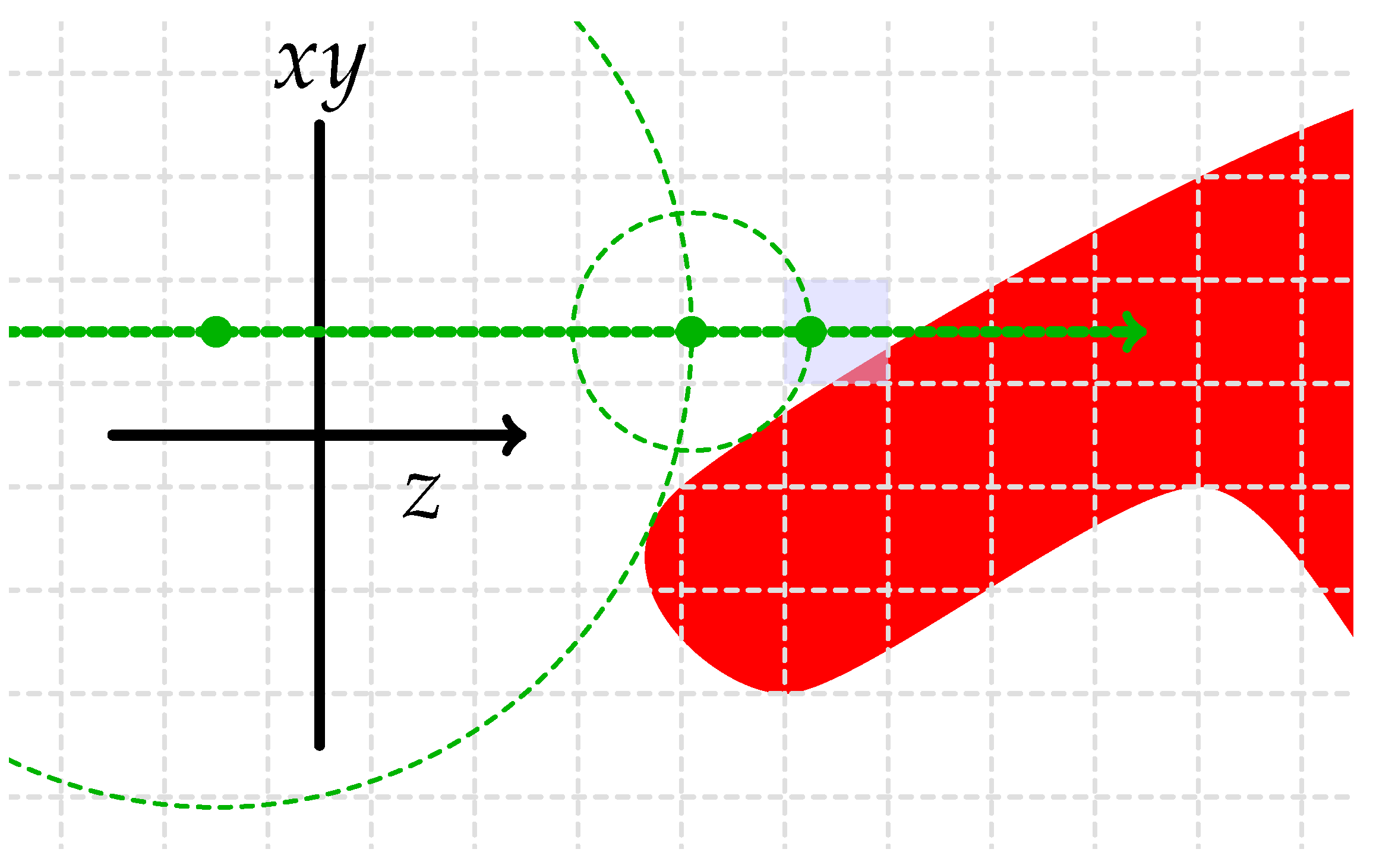
  • We describe a fast algorithm for polygonizing SDBs based on sphere tracing (ray marching).
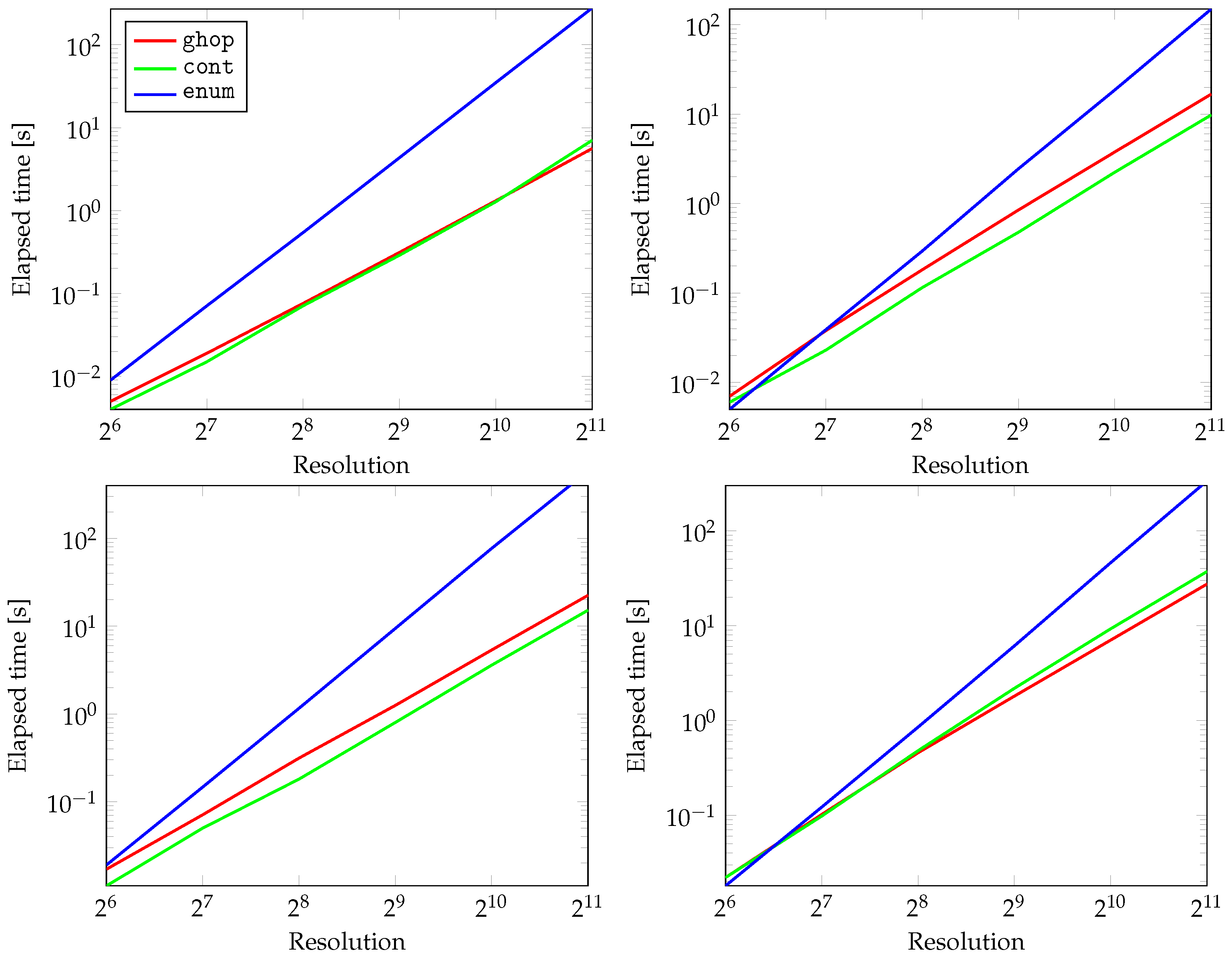
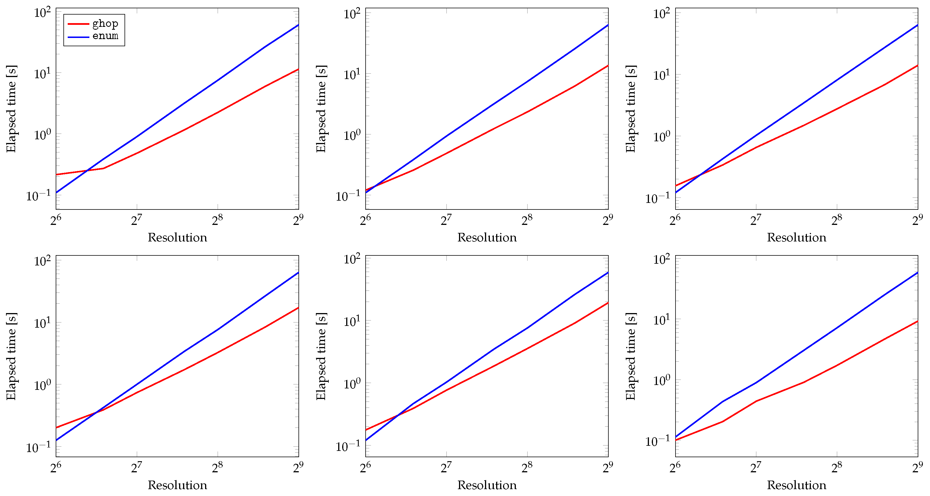
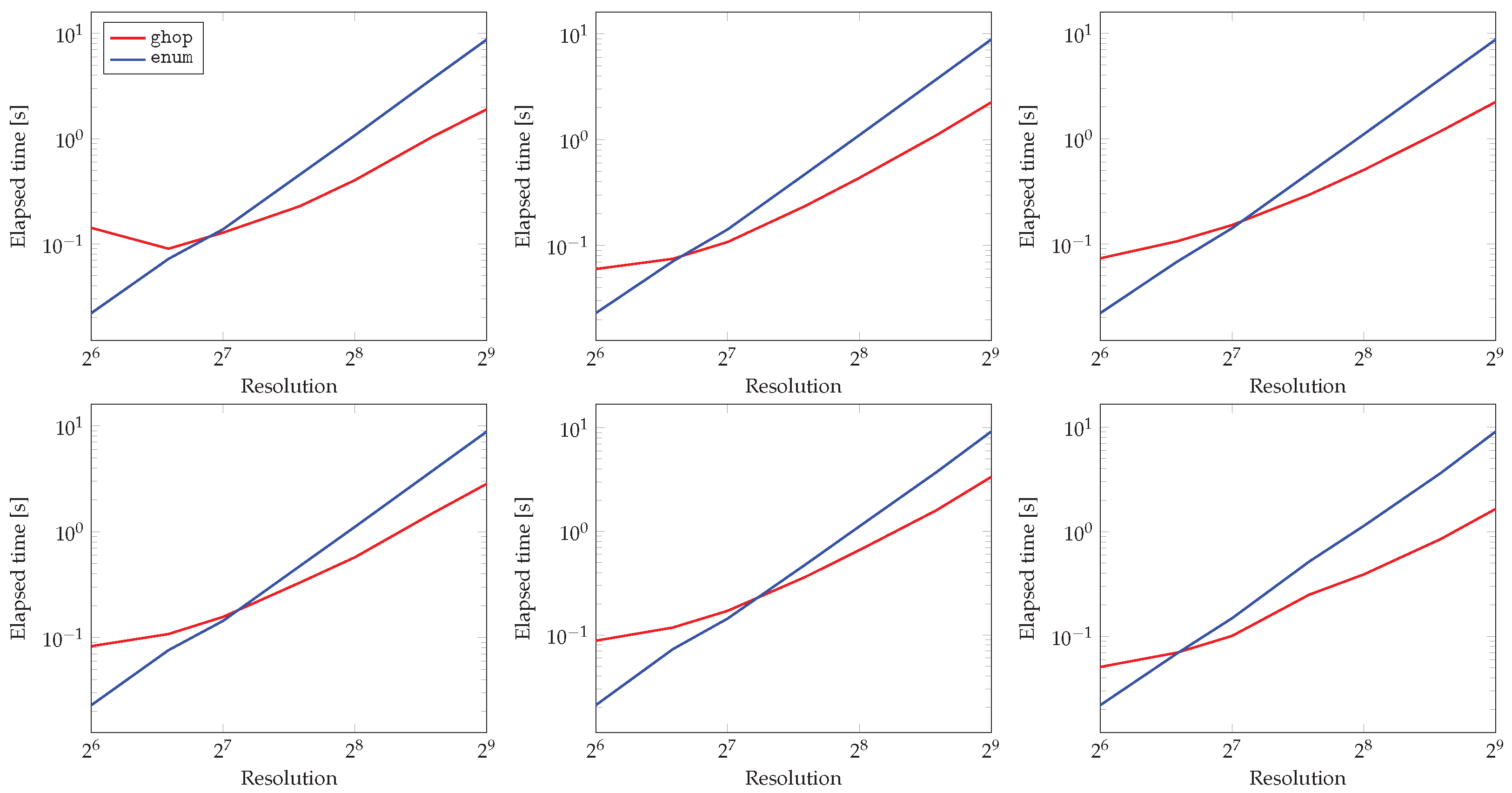
  • We theoretically show that this algorithm is asymptotically faster than the obvious approaches (e.g., marching cubes [10] over the whole grid).
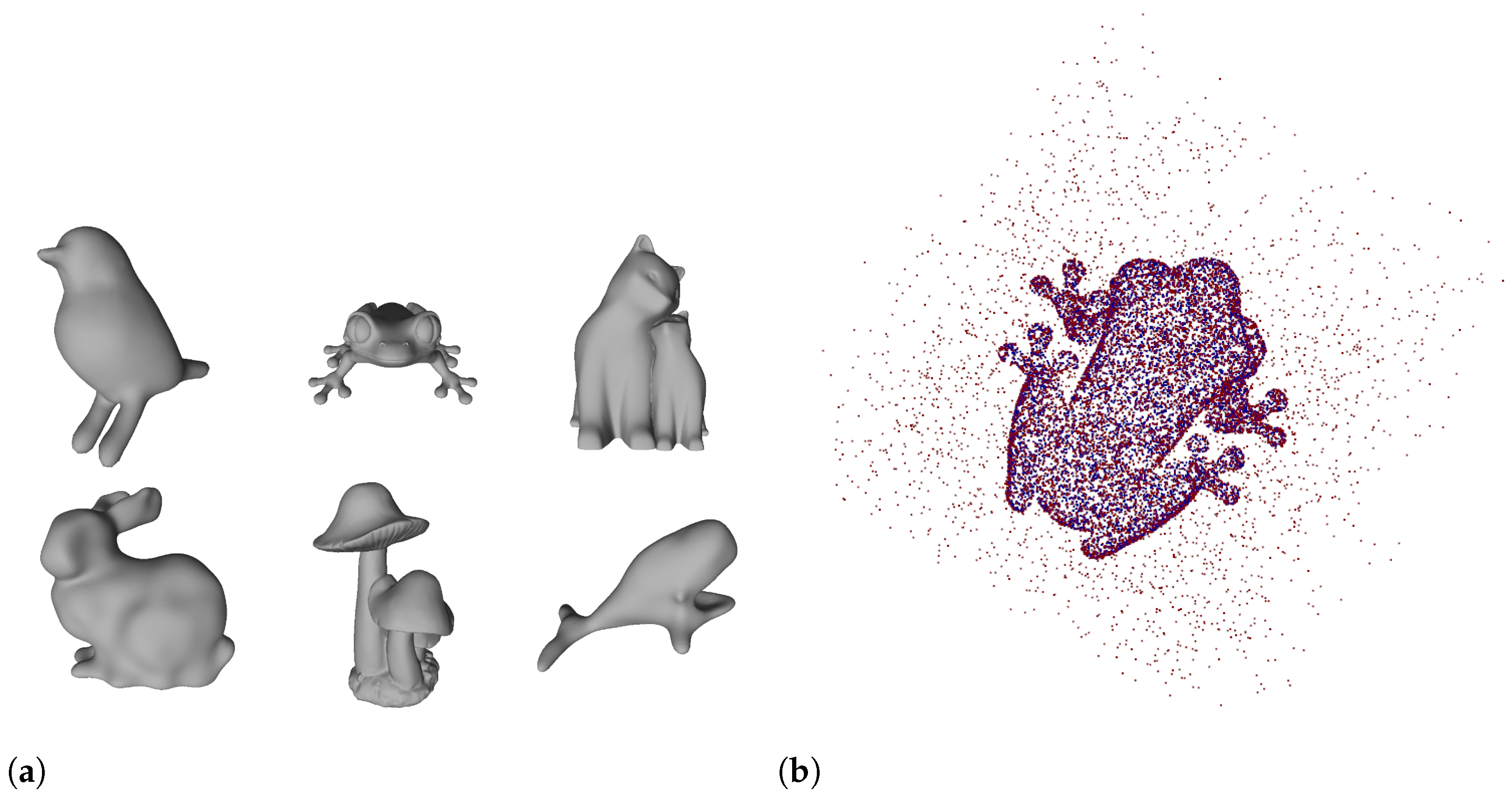
  • We empirically confirm this in practice for signed distance bounds encoded with deep neural networks.
The next section provides context, basic definitions, and related prior work. The description of our method and its analysis/comparisons follow after that.

2. Basic Definitions and Related Work

In our case, the polygonization volume is an axis-aligned cube centered at the origin. The shape represented by its SDB is withing this cube. This cube is partitioned into a rectangular grid with N 3 cells by subdividing each of its sides into N intervals of equal size. If we assume we are not dealing with fractals, only O ( N 2 ) cells asymptotically contain the surface of our shape. Thus, the only triangles that need to be computed are passing through these cells. This puts the lower bound on the complexity of the triangularization algorithm. However, the challenge is to isolate just these O ( N 2 ) cells.
The simplest solution, which leads to O ( N 3 ) complexity, is to check each of the N 3 cells. This process is called enumeration [11] (Section 4.2.2 in the book), and for some purposes it is too slow. The original applications of the marching cubes algorithm [10] applied this slow approach. However, these applications usually dealt with real-world data obtained through measurements (e.g., CT scans), not well defined mathematical objects.
An improvement to this basic enumeration scheme is known as continuation [11] (Section 4.2.3 in the book). The idea of this approach is quite simple. Starting from a single “seed” cell that intersects the surface of the shape, new cells are propagated across the surface until the entire surface is enclosed. The complexity of this algorithm is O ( N 2 ) because only the surface cells are analyzed. Thus, we also call it surface tracing/crawling. Its main disadvantage is that it produces a single mesh component for each seed cell, i.e., we need a separate seed cell to polygonize all disjoint shape components. This can be problematic in practice. Another issue with this approach is caused by the limited numerical precision of digital computers when representing seed cell parameters (e.g., their center point coordinates)—this complicates the positioning of the seed cell. Of course, these problems only show up for high grid resolutions, i.e., large values of N.
We also mention the unpublished work of Christopher Olah [12,13]. This method aims at similar goals (transform an SDB into a triangle mesh) but uses a different subdivision strategy over the grid (recursive partitioning instead of sphere tracing), and no detailed complexity analysis was performed. It is not a formal academic work but an implementation.
Besides the mentioned work that warrants a direct experimental comparison (enumeration and continuation [11], marching cubes [10]) to our method, we also mention more broad work for additional context. There are a number of algorithms for speeding up isosurface extraction (as polygon meshes) from real-world data such as MRI and CT scans, e.g., based on octrees [14] or other, more exotic data structures [15,16]. However, these methods assume that data points on the grid are already known (sampled). Thus, direct application of these algorithms to polygonizing SDBs is not possible.
There is also a large body of work on generative models for geometry. In this context, we mention those that directly output polygons. Gao et al. [17] represent geometry as a signed distance field defined on a deformable tetrahedral grid and incorporate this into a learning framework. Their end result is a neural representation that can directly generate polygonal models from the training data distribution. In the PolyDiff paper [18], the authors introduce a mesh generator based on a denoising diffusion process [19,20]. In the MeshGPT paper [21], the authors use a decoder-only transformer neural network to directly output the polygons of a mesh. All these works are learning-based, i.e., require a large dataset in order to be effective, are not easy to implement/use in a production system like a game engine, and require significant computational resources.
The next section provides a detailed (mathematical, algorithmic) description of the gridhopping method to enable its analysis.

3. Method

Another way to speed up the triangularization process is to apply a variant of ray marching called sphere tracing (described by John C. Hart [1,2]). Note that sphere tracing is originally a 3D rendering scheme. However, we repurpose it here for polygonization. The basic idea is to define a ray and move along its direction until we find the intersection with the shape or exit the rendering volume. In sphere tracing, the marching step is set to be equal to the (estimated) distance of the current point to the shape. This approach greatly speeds up the process of finding the intersection. However, unlike in the ray marching-based rendering of images, we do not stop the marching process at the surface. The marching along the ray in continued (starting at the next cell along the direction of the ray) until the end of the polygonization volume is reached. Let us call this method gridhopping. This process enables us to efficiently isolate the O ( N 2 ) cells that contain the surface of the shape: we present theoretical and experimental evidence that this method extracts a triangle mesh from a signed distance bound in O ( N 2 log N ) steps for a grid with N 3 cells. Note that this is a significant speed improvement over the basic approach that analyzes each of the N 3 cells, leading to O ( N 3 ) complexity.
Without loss of generality, we assume that our polygonization volume is a unit cube centered at the origin. The grid resolution is specified by N: there are N 3 cubic cells in the grid, each with a volume equal to 1 N 3 . Each cell is assigned a triplet of integers ( i , j , k ) , with i , j , k { 0 , 1 , 2 , , N 1 } . The centroids of the cells are computed according to the following rules:
x i = 1 2 + 1 2 N + i N y j = 1 2 + 1 2 N + j N z k = 1 2 + 1 2 N + k N
A total of N 2 rays are cast in the + z direction from the plane z = 0.5 + 1 2 N . Such rays have the following vector parameterization for λ 0 :
R i j r = o i j + λ d
where o i j = ( x i , y j , 0.5 + 1 2 N ) T is the origin of ray R i j and d = ( 0 , 0 , 1 ) T is its direction. The ( x i , y j ) pairs ( N 2 of them) are computed according to Equation (1).
We move along each ray using the ray marching (sphere tracing) [1,2] method. If the polygonization volume contains a shape S described by its signed distance bound f S , the following iteration describes this process:
r n + 1 = r n + f S ( r n ) d
The iteration starts at r 0 = o i j and continues until f S ( r n ) is sufficiently small (indicating we are very close to the surface of S, by definition of f S ). In our case, we are only interested in moving close enough to the surface to determine the ( i , j , k ) triplet determining the cell. Simple algebra shows that a cell possibly intersects the surface of S, and we have to call it a polygonization routine if the distance f S is less than or equal to
1 2 N 2 + 1 2 N 2 + 1 N 2 = 6 2 N
The pseudocode in Algorithm 1 contains the details, and Figure 1 provides a visual summary/illustration.
Algorithm 1 Pseudocode for the gridhopping method
// inputs :
// ∗ ‘eval_sdb’ is the signed distance bound represeting a shape
// ∗ ‘N’ is the grid resolution
function apply_grid_hopping (eval_sdb, N)
{
for (int i = 0; i < N; ++i)
  for (int j = 0; j < N; ++j)
  {
   int k = 0;
   while (true)
   {
    // set the origin of the ray
    float x = −1.0/2.0 + 1.0/(2.0∗N) + i/N;
    float x = −1.0/2.0 + 1.0/(2.0∗N) + j/N;
    float x = −1.0/2.0 + 1.0/(2.0∗N) + k/N;
    // use ray marching to determine how much to move along the ray
    float t = trace_ray (
     [x, y, z],                              // origin of the ray
     [0.0, 0.0, 1.0],                    // direction of the ray
     eval_sdb,                           // signed distance bound
     1.05∗(1.0/2.0 − z),              // max distance to travel
     Math . sqrt (6.0)/(2.0∗N) // distance to surface we require
    );
    // set the new value of z and its associated cell, (i, j, k)
    z = z + t;
    k = Math . floor (N∗(z + 1.0/2.0 − 1.0/(2.0∗N)));
    // are we outside the polygonization volume?
    if (k > N − 1 || z > 1.05/2.0)
     break;
    // polygonize cell (i, j, k)
    … // <- polygonizaiton code goes here, e.g., Marching cubes
    // move further along the z direction
    ++k;
   }
  }
}
If the ray intersects the surface and we denote the closest intersection to r 0 with r * , then the above iteration converges to r * . This is because of the following:
  • f S ( r n ) 0 ;
  • On the ray between r 0 and r * , f S ( r ) = 0 only for r = r * ;
  • The iteration will never “overshoot” r * because f S is a signed distance bound.
See [1] for additional analysis.

4. Theoretical Analysis of Computational Complexity

We analyze the asymptotic number of steps required by the method from the previous section to polygonize a shape defined through its signed distance bound. For nonfractal shapes, there are at most O ( N 2 ) cells that contain polygons. The challenge is to isolate these cells in a fast manner. The trivial way is to check all N 3 cells. This may be too slow for some applications when high resolution (large N) is required. Our claim is that the algorithm from the previous section is faster than that: its complexity is O ( N 2 log N ) .
We provide evidence for this in the following steps:
  • Provide a proof for polygonizing planes;
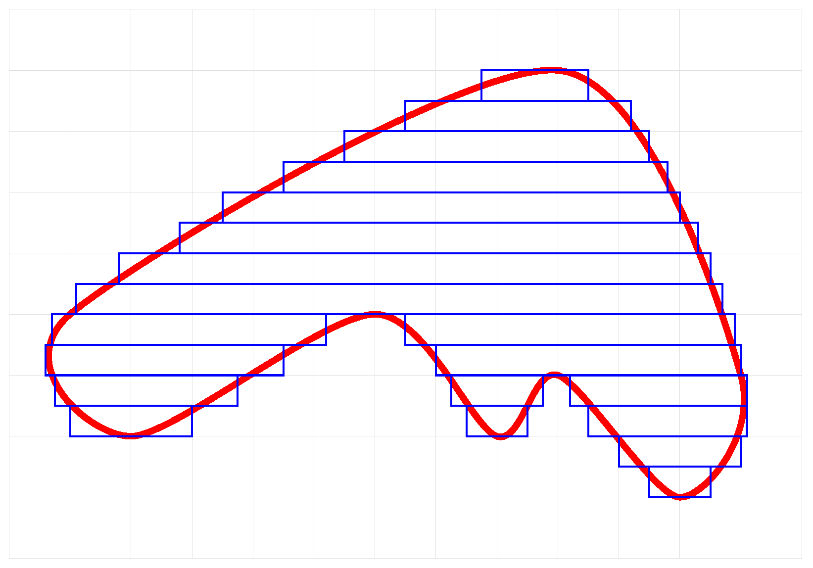
  • Provide a proof for polygonizing axis-aligned boxes;
  • Argue that any nonfractal shape can be approximated as a union of boxes.
These steps are explained in the following three subsections.

4.1. Polygonizing Planes

A plane is a flat, two-dimensional surface that extends infinitely far. Of course, we are interested in polygonizing only the part that intersects with the polygonization volume.
The exact signed distance from a point r to a plane P is given by the following Equation [22]:
D P ( r ) = n P T · ( r r P ) ,
where r P is some point lying on P and n P is P’s normal vector such that n P T · n P = | | n P | | 2 2 = 1 .
We analyze three different cases: two cases of axis-aligned planes and one case for a plane in a general position. The first case is when the plane and the rays are perpendicular. In our case, since the rays are cast in the + z direction, this corresponds to the plane z = C for some constant C. The second case is when the plane and the rays are parallel (plane specified by x = C or y = C ). The third case is the plane in a general position.
Case #1: plane P and rays are perpendicular. First, notice that the orientation of the plane does not matter since the ray marching always uses the absolute value of the computed distance bound. Thus, we have two subcases: approaching the plane and escaping the vicinity of its surface. The approaching phase is performed in a single step for each ray since D P provides the exact distance estimate. Hence, its complexity is O ( 1 ) , independent of N, the position of the plane along the z axis, and the starting point. Since there are N 2 rays, the complexity of the approaching phase is O ( N 2 ) . Escaping the plane’s surface requires more work, and the following analysis holds for each of the N 2 rays that need to be cast. Let r 0 denote the starting point in the vicinity of P’s surface. Note that D P ( r 0 ) is about 1 N in size immediately after the polygonization routines for P’s cells have been invoked (at most two in this case, only one containing polygons). Analyzing the iteration (3), it is easy to see that D P ( r 1 ) = 2 · D P ( r 0 ) , and in general, the following holds:
D P ( r n ) = 2 n · D P ( r 0 ) ,
i.e., the method escapes the surface in steps of exponentially increasing size. If D P ( r 0 ) is about 1 N , then the number of steps required to exit the polygonization volume is O ( log N ) . Given that there are N 2 such rays, the complexity of the escaping phase is O ( N 2 log N ) . The approaching and escaping phase are performed sequentially. Thus, the complexity of polygonizing a plane in this scenario is O ( N 2 log N ) .
Case #2: plane P and rays are parallel. First, notice that if the distance between a ray and P is equal to k N in this case, then the method exits the polygonization volume in approximately N k steps. There are N rays marching through cells that contain P. The algorithm takes approximately N steps along each of these rays before terminating. Next, notice that there are N rays above and N rays below P, parallel to P, and of distance approximately k N to P for some integer k < N . These rays require about N / k steps before exiting the polygonization volume. Thus, a conservative estimate for the number of steps S for all N 2 rays is
S N 2 + 2 N 2 + N 2 2 + N 2 3 + + N 2 N 1 + N = N 2 · 1 + 2 H N ,
where H N is Nth partial sum of the harmonic series [23]: H N = n = 1 N 1 n . The number H N is about as large as log N . The reason for this comes from the comparison of H N and the integral 1 N 1 x d x , which can be solved analytically. Thus, it follows that S O ( N 2 log N ) and the complexity of case #2 is O ( N 2 log N ) .
Case #3: the general case. Due to easier exposition and without loss of generality, we assume that the plane passes through origin (i.e., r P = 0 ). Combining this assumption with Equations (3) and (5), we obtain the following iteration for the z coordinate:
z n + 1 = z n + n x x 0 + n y y 0 + n z z n
where ( n x , n y , n z ) T is the unit normal of the plane and ( x 0 , y 0 , z 0 ) T is the origin of the ray. Let us denote with z * the intersection of the ray and the plane:
z * = n x x 0 + n y y 0 n z
Without loss of generality, we assume that n z < 0 . There are two subcases: (1) the method approaches the plane along the ray and (2) the method moves away from the plane along the ray. In the first subcase, we have n x x 0 + n y y 0 + n z z n > 0 . In this scenario, it is easy to see that
z * z n = ( 1 + n z ) · ( z * z n 1 ) = = ( 1 + n z ) n ( z * z 0 )
Since 1 + n z is between 0 and 1, we have that the number of iterations n has to be about O ( log N ) so that D P ( r n ) becomes less than 6 2 N (at which point the polygonization routine is invoked and we can move to the other side of the plane). In the second subcase, we have n x x 0 + n y y 0 + n z z n < 0 . Now the following holds:
z n z * = ( 1 n z ) · ( z n 1 z * ) = = ( 1 n z ) n ( z 0 z * )
Since 1 n z is greater than 1, at most O ( log N ) iterations along the ray are needed to exit the polygonization volume. Given that there are N 2 rays in total, the complexity of case #3 is O ( N 2 log N ) .

4.2. Polygonizing Rectangular Boxes

A rectangular box can be obtained by intersecting six axis-aligned planes. Let d 1 , d 2 , , d 6 be the distances from point ( x , y , z ) to each of these planes. Then the distance to the box is bounded by
f ( x , y , z ) = max { d 1 , d 2 , d 3 , d 4 , d 5 , d 6 }
Since polygonizing each of the box sides takes O ( N 2 log N ) steps, this is also the total complexity of polygonizing a box.
This can also be justified by the fact that the max operation partitions the polygonization volume into several regions. In each of these regions, only the distance to one particular plane is relevant (largest d i ). All the rays passing through this region require at most O ( N 2 log N ) steps before exiting the region. The conclusion about the total complexity follows from the fact that the number of such regions is finite.
As noted, Equation (12) bounds the distance to the box. The exact distance function can be constructed, and this leads to more efficient marching in practice (a constant speed-up, not in the asymptotic sense) (for example, see https://www.youtube.com/watch?v=62-pRVZuS5c (accessed on 26 February 2024)).

4.3. Polygonizing Other Shapes

A shape can be approximated by K axis-aligned boxes. See Figure 2 for an illustration of this process.
Of course, we can improve the quality of approximation by increasing K. It is important to note that K does not depend on grid resolution N. The efficiency of approximation can be increased by using non-axis-aligned planes at the boundary of the shape. This process is not unlike the use of triangle meshes in modern computer graphics.
Approximating the shape as a union of K boxes keeps the O ( N 2 log N ) polygonization complexity. This is because the union of K boxes (and, in general, shapes) can be obtained by applying the min operation to combine all the individual distance bounds. The number of steps the method has to make in this case is asymptotically no worse than polygonizing each box on its own. Thus, the total number of steps scales as O ( N 2 log N ) since the grid resolution N does not depend on K.

5. Experimental Analysis

In this section, we experimentally compare the three methods (refer to Section 2 for the overview of the methods): gridhopping (ghop), enumeration (enum), and continuation (cont). The goal is to show that the enum method is asymptotically slower than cont and ghop.
The polygonization of a cell is obtained with the marching cubes algorithm. To achieve this, we implement all methods and run them on different scenes for varying grid resolutions. It is important to note that all implementations produce exactly the same meshes when polygonizing signed distance bounds.

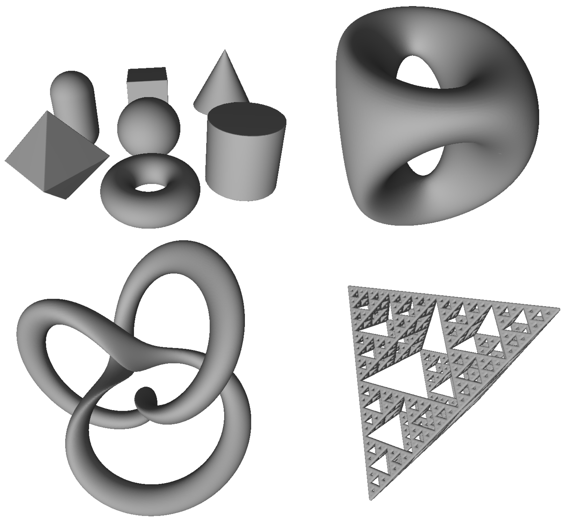
5.1. Primitives and Simple Shapes

We use four different scenes in this batch of experiments. The first scene contains seven basic primitives: sphere, cube, cone, cylinder, torus, hexagonal prism, and capsule. All these primitives have simple and efficient signed distance bounds. The second scene is a surface of genus 2 given by the implicit equation 2 y ( y 2 3 x 2 ) ( 1 z 2 ) + ( x 2 + y 2 ) 2 ( 9 z 2 1 ) ( 1 z 2 ) = 0 . The third scene contains a knot with an explicit signed distance bound. The fourth scene contains the Sierpinski tetrahedron. These scenes are visualized in Figure 3.
Figure 4 shows the times needed to polygonize the scenes with the slow and the fast algorithms.
Note that the axes in the graphs have logarithmic scale.
We can see that the measured times for both methods appear as lines. This is expected since the computed theoretical complexities are polynomial ( N 3 and N 2 ). However, the fast method becomes significantly faster for large N, i.e., asymptotically. This aligns with the predictions from Section 4.

5.2. Experiments on Learned SDBs

There has been considerable interest in learning-based methods for signed distance bound modelling. Furthermore, this is lately especially true in the area of deep learning [3,4,5,7,8,24,25,26,27] (see section “Implicit representation” at https://github.com/subeeshvasu/Awsome_Deep_Geometry_Learning (accessed on 26 February 2024) for more (and updated) examples).
Let us constrict our analysis to a set of methods that use a neural network (NN) to approximate an SDB of a shape:
NN θ ( x , y , z ) d S ( x , y , z ) ,
where ( x , y , z ) R 3 is a point in 3D space and d S ( x , y , z ) denotes its Euclidean distance to the surface of the shape S. The parameters of the N N are denoted with θ . These parameters have to be tuned to make the approximation as best as possible.
Our hypothesis is that gridhopping is a faster algorithm for transforming such neural SDBs to triangle meshes than the basic enumeration technique is. This should especially be true for higher grid resolutions.
To experimentally test our claim, we take six shapes from the Thingi10K dataset [28] (see Figure 5a).
These shapes are represented as triangle meshes, and we need their SDBs. We first sample a dataset of point–distance pairs around each shape (sampling algorithm by Park et al. [5], implementation: https://github.com/marian42/mesh_to_sdf (accessed on 26 February 2024)):
{ ( x i , y i , z i ) , d i } i = 1 S
An example can be seen in Figure 5b.
Next, we use the Adam stochastic gradient descent technique to tune θ (from Equation (13)) so that NN θ ( x i , y i , z i ) d i . The NN architecture is very simple: eight layers, each with an embedding dimension equal to 64, and the ReLU is set as the activation function. To speed up training, we also use batch normalization in all layers except the last one. This results in about 30 , 000 network weights (120 kB of memory). By modern standards, this is a tiny network, but it is capable of accurately representing the shapes used in our experiments. Note that our methodology trivially extends to other NN approaches for SDB modelling. We decided to go with this one to keep things as simple as possible.
Recall that if certain criteria are not met (e.g., Lipschitz continuity), sphere tracing might “miss” parts of the surface of the shape, and we obtain an incomplete mesh with gridhopping [1]. In practice, this means that the NN overestimates the surface distance for some points (e.g., due to the imperfection of the learning algorithm). To circumvent these problems, we shrink the signed distance approximation by factor λ : SDB ( x , y , z ) = NN θ ( x , y , z ) λ . This procedure slows down gridhopping and has no effects on the speed of the complete enumeration algorithm. We empirically found that λ = 1.5 works well. This (or a smaller) value results in perfect mesh reconstructions for all shapes, i.e., all methods produce identical meshes.
We compare the times needed to polygonize the prepared SDBs for the complete enumeration algorithm and gridhopping. The grid resolution N varies from 64 to 512. First, all computations are performed on an Intel(R) Core(TM) i7-9750H CPU @ 2.60GHz. Batching the NN evaluations in chunks of size 10 , 000 leads to significant speed improvements for both methods. The results can be seen in Figure 6.
Even though the enumeration method is sometimes faster for small grid resolutions, we can clearly observe that gridhopping has a significant asymptotic advantage. The results are in accordance with the theoretically predicted ones in Section 4: N 3 vs. N 2 computational complexity.
We also performed experiments when computations are performed on an Nvidia GeForce RTX 2060 Mobile GPU. Batching the NN computations in chunks of size 100 , 000 seems best, and we report timings in this setting, Figure 7.
The theoretical complexity results hold in this setting as well. Furthermore, GPU computations are significantly faster than CPU ones. However, gridhopping is somewhat slower for smaller grid resolutions. We attribute this fact to the constant overhead needed to prepare the gridhopping run.

6. Conclusions

In this work, we described and evaluated gridhopping—a method for transforming shapes defined by signed distance bounds into triangle meshes. Its main advantages are simplicity, ease of implementation, and processing speed. We confirmed this in theory and experiments by comparing the method to the enumeration and continuation variants of the marching cubes algorithm [10], which are the standard approaches for polygonizing signed distance bounds in practical applications. We used both simple shapes defined by short equations/code and more complicated ones defined through neural networks. We also showed that these conclusions hold when the computations are performed on a CPU and on a GPU, which is a further confirmation of the practicality of the method.
The main limitations of gridhopping are the Lipschitz continuity requirement; that it works only with abstract, mathematically defined shapes and not real-world data like point clouds; and the fact that it generates too many triangles for some simple shapes. Note that the last limitation also holds for marching cubes, as both methods produce identical triangle meshes. Furthermore, within the context of this paper, we would like to mention that the marching cubes-based pipelines (gridhopping included) might be competing with deep learning-based methods that generate triangle meshes [18,21], especially if the texture is included [17]. However, these deep learning-based approaches are not practical in many situations due to their implementation complexity, large processing speed, and the requirement for high-quality training data to be effective. Therefore, gridhopping is still relevant for the wider engineering community.
Our implementation of the gridhopping method is available at https://github.com/nenadmarkus/gridhopping (accessed on 26 February 2024).

Author Contributions

Conceptualization, methodology, software, writing: N.M. Review, editing, validation, funding acquisition: M.S. All authors have read and agreed to the published version of the manuscript.

Funding

This research was supported by the Croatian National Recovery and Resilience Plan (NPOO) under the project Research and Development of Multiple Innovative Products, Services and Business Models Aimed at Strengthening Sustainable Tourism and the Green and Digital Transition of Tourism (ROBOCAMP), with grant number NPOO.C1.6.R1-I2.01. Furthermore, work was supported by the European Union under the project Enhanced Pilot Interfaces & Interactions for fighter Cockpit (EPIIC) funded by European Defence Fund (EDF) Grant Agreement 101103592.

Data Availability Statement

The original contributions presented in the study are included in the article, further inquiries can be directed to the authors.

Conflicts of Interest

The authors declare no conflicts of interest. The funding sponsors had no role in the design of the study; in the collection, analyses, or interpretation of data; in the writing of the manuscript, and in the decision to publish the results.

References

  1. Hart, J.C. Sphere Tracing: A Geometric Method for the Antialiased Ray Tracing of Implicit Surfaces. Vis. Comput. 1994, 12, 527–545. [Google Scholar] [CrossRef]
  2. Hart, J.C.; Sandin, D.J.; Kauffman, L.H. Ray Tracing Deterministic 3-D Fractals. In ACM SIGGRAPH Computer Graphics; Association for Computing Machinery: New York, NY, USA, 1989. [Google Scholar]
  3. Davies, T.; Nowrouzezahrai, D.; Jacobson, A. Overfit Neural Networks as a Compact Shape Representation. arXiv 2020, arXiv:2009.09808. [Google Scholar]
  4. Chen, Z.; Zhang, H. Learning Implicit Fields for Generative Shape Modeling. In Proceedings of the CVPR, Long Beach, CA, USA, 15–20 June 2019. [Google Scholar]
  5. Park, J.J.; Florence, P.; Straub, J.; Newcombe, R.; Lovegrove, S. DeepSDF: Learning Continuous Signed Distance Functionsfor Shape Representation. In Proceedings of the CVPR, Long Beach, CA, USA, 15–20 June 2019. [Google Scholar]
  6. Li, L.; Sung, M.; Dubrovina, A.; Yi, L.; Guibas, L. Supervised Fitting of Geometric Primitives to 3D Point Clouds. In Proceedings of the CVPR, Long Beach, CA, USA, 15–20 June 2019. [Google Scholar]
  7. Duggal, S.; Wang, Z.; Ma, W.C.; Manivasagam, S.; Liang, J.; Wang, S.; Urtasun, R. Secrets of 3D Implicit Object Shape Reconstruction in the Wild. arXiv 2021, arXiv:2101.06860. [Google Scholar]
  8. Hao, Z.; Averbuch-Elor, H.; Snavely, N.; Belongie, S. DualSDF: Semantic Shape Manipulation using a Two-Level Representation. In Proceedings of the CVPR, Long Beach, CA, USA, 15–20 June 2020. [Google Scholar]
  9. Wu, Y.; Man, J.; Xie, Z. A double layer method for constructing signed distance fields from triangle meshes. Graph. Model. 2014, 76, 214–223. [Google Scholar] [CrossRef]
  10. Lorensen, W.E.; Cline, H.E. Marching cubes: A high resolution 3D surface construction algorithm. In ACM SIGGRAPH Computer Graphics; Association for Computing Machinery: New York, NY, USA, 1987. [Google Scholar]
  11. Bloomenthal, J. (Ed.) Introduction to Implicit Surfaces; Morgan-Kaufmann: Burlington, MA, USA, 1997. [Google Scholar]
  12. Olah, C. Manipulation of Implicit Functions with an Eye on CAD, 2011. Available online: https://christopherolah.wordpress.com/2011/11/06/manipulation-of-implicit-functions-with-an-eye-on-cad/ (accessed on 26 February 2024).
  13. Olah, C. ImplicitCAD, 2011. Available online: https://github.com/Haskell-Things/ImplicitCAD (accessed on 26 February 2024).
  14. Wilhelms, J.; Gelder, A.V. Octrees for faster isosurface generation. Trans. Graph. 1992, 11, 201–227. [Google Scholar] [CrossRef]
  15. Cigoni, P.; Marino, P.; Montani, C.; Puppo, E.; Scopigno, R. Speeding Up Isosurface Extraction Using Interval Trees. IEEE Trans. Vis. Comput. Graph. 1997, 3, 158–170. [Google Scholar] [CrossRef]
  16. Livnat, Y.; Shen, H.W.; Johnson, C.R. A Near Optimal Isosurface Extraction Algorithm Using the Span Space. IEEE Trans. Vis. Comput. Graph. 1996, 2, 73–84. [Google Scholar] [CrossRef]
  17. Gao, J.; Shen, T.; Wang, Z.; Chen, W.; Yin, K.; Li, D.; Litany, O.; Gojcic, Z.; Fidler, S. GET3D: A Generative Model of High Quality 3D Textured Shapes Learned from Images. In Proceedings of the Advances in Neural Information Processing Systems, New Orleans, LA, USA, 28 November–9 December 2022. [Google Scholar]
  18. Alliegro, A.; Siddiqui, Y.; Tommasi, T.; Nießner, M. PolyDiff: Generating 3D Polygonal Meshes with Diffusion Models. arXiv 2023, arXiv:2312.11417. [Google Scholar]
  19. Sohl-Dickstein, J.; Weiss, E.; Maheswaranathan, N.; Ganguli, S. Deep Unsupervised Learning using Nonequilibrium Thermodynamics. In Proceedings of the ICML, Lille, France, 6–11 July 2015. [Google Scholar]
  20. Ho, J.; Jain, A.; Abbeel, P. Denoising Diffusion Probabilistic Models. arXiv 2020, arXiv:2006.11239. [Google Scholar]
  21. Siddiqui, Y.; Alliegro, A.; Artemov, A.; Tommasi, T.; Sirigatti, D.; Rosov, V.; Dai, A.; Nießner, M. MeshGPT: Generating Triangle Meshes with Decoder-Only Transformers. arXiv 2023, arXiv:2311.15475. [Google Scholar]
  22. Weisstein, E.W. Point-Plane Distance. From MathWorld—A Wolfram Web Resource. Available online: https://mathworld.wolfram.com/Point-PlaneDistance.html (accessed on 26 February 2024).
  23. Weisstein, E.W. Harmonic Series. From MathWorld—A Wolfram Web Resource. Available online: https://mathworld.wolfram.com/HarmonicSeries.html (accessed on 26 February 2024).
  24. Yao, S.; Yang, F.; Cheng, Y.; Mozerov, M.G. 3D Shapes Local Geometry Codes Learning with SDF. In Proceedings of the ICCV Workshops, Montreal, BC, Canada, 11–17 October 2021. [Google Scholar]
  25. Yifan, W.; Rahmann, L.; Sorkine-Hornung, O. Geometry-Consistent Neural Shape Representation with Implicit Displacement Fields. arXiv 2021, arXiv:2106.05187. [Google Scholar]
  26. Mu, J.; Qiu, W.; Kortylewski, A.; Yuille, A.; Vasconcelos, N.; Wang, X. A-SDF: Learning Disentangled Signed Distance Functions for Articulated Shape Representation. arXiv 2021, arXiv:2104.07645. [Google Scholar]
  27. Takikawa, T.; Litalien, J.; Yin, K.; Kreis, K.; Loop, C.; Nowrouzezahrai, D.; Jacobson, A.; McGuire, M.; Fidler, S. Neural Geometric Level of Detail: Real-time Rendering with Implicit 3D Shapes. In Proceedings of the CVPR, Nashville, TN, USA, 20–25 June 2021. [Google Scholar]
  28. Zhou, Q.; Jacobson, A. Thingi10K: A Dataset of 10,000 3D-Printing Models. arXiv 2016, arXiv:1605.04797. [Google Scholar]
Figure 1. A 2D illustration of the gridhopping method: grid cells are dashed gray squares, the shape with an SDF is in red, and the z axis and the x y plane are in black. The dashed green line (parallel to the z axis) represents one of the rays along which sphere tracing is applied. Since the SDF of the red shape is known, we can compute the maximum step size along the ray (green circles). The green dots are locations obtained from these calculations. The marching cubes polygonization is first applied to the light-blue cell since it is the first one along the ray that satisfies the condition related to Equation (4).
Algorithms 17 00137 g001
Figure 2. One possible approximation of a shape (red) as a union of axis-aligned boxes (blue). Note that the approximation would be much more efficient if non-axis-aligned planes are used on the boundary.
Algorithms 17 00137 g002
Figure 3. The four scenes used in our experiments from Section 5.1.
Algorithms 17 00137 g003
Figure 4. Elapsed times plotted against grid resolution for the four different scenes from Figure 3. The legend for all graphs is plotted in the top left one. Note that all axes are logarithmic.
Algorithms 17 00137 g004
Figure 5. Figures to help understand our experiments with deep learning-based SDBs. (a) Shapes from Section 5.2. (b) A generated point cloud.
Algorithms 17 00137 g005
Figure 6. CPU experiments: elapsed times plotted against grid resolution for the six different shapes from Figure 5a. The legend for all graphs is plotted in the top left one. Note that all axes are logarithmic.
Algorithms 17 00137 g006
Figure 7. Same setting as in Figure 6 except the computations are performed on the GPU.
Algorithms 17 00137 g007
Disclaimer/Publisher’s Note: The statements, opinions and data contained in all publications are solely those of the individual author(s) and contributor(s) and not of MDPI and/or the editor(s). MDPI and/or the editor(s) disclaim responsibility for any injury to people or property resulting from any ideas, methods, instructions or products referred to in the content.

