1. Introduction
In the past few decades, China has become one of the largest economies in the world. Its progress has attracted the interest of researchers from business, government, and academia. For Western researchers, there is an increasing interest in accessing Chinese media sources and increasing knowledge of China’s culture, economy, and intellectual systems as China’s influence on the world grows [
1]. A challenge in this is the large volume of publications originating from China, a country of over a billion people, as well as the challenge of non-native Chinese readers evaluating Chinese news.
These researchers of Chinese media, faced with the daunting task of sorting through a flood of news articles, would benefit from natural language processing (NLP) techniques to categorize news articles in their topics of interest. An experienced researcher can accomplish a lot on the Internet with a search engine and any one of the many translation tools available, which leverage natural language processing in several different ways. However, the sources are so numerous that a search engine’s index could lack records of the newest, most relevant articles, which could lead to missed opportunities for the researcher [
2]. A web scraper with a means to evaluate headlines of articles would be a means to rapidly select relevant, timely articles for researcher review.
In order to automate the classification of Chinese-language news headlines, this paper will use the cross-industry standard process for data mining (CRISP-DM) to investigate how NLP techniques, along with AI/ML models, can be applied toward this goal. Standardized metrics and processes will be used to compare the performance of each technique and each model. The accurate classification of headlines can enable researchers to prioritize reviews of the numerous articles appearing on Chinese news websites. Other components involved in the process will not be covered here, such as aggregating headlines through web scraping, translating the headline and article after selection, and other functions that enable the actual reviewing of the Chinese language content. Investigated models will be evaluated to provide options for integration into either a lightweight computing environment or one that is more resource-intensive.
1.1. Data Understanding
Jinri Toutiao, or “Today’s Headlines”, is a Chinese news site that aggregates and analyzes article content based on user profiles to tailor news feeds for each user [
3]. As part of the process, they classify articles into categories. The publicly available Toutiao dataset selected for this study possesses 382,688 headlines, which are tagged as one of 15 news topic categories, such as finance or culture [
4]. Selected rows from the dataset are shown in
Table 1, presenting the category and headline fields from the dataset. The headline’s translation is also shown, along with notes that highlight occurrences of duplicate entries, entries that are partially English, and entries that are completely English. Chinese-only entries consist of 99.989% of the dataset.
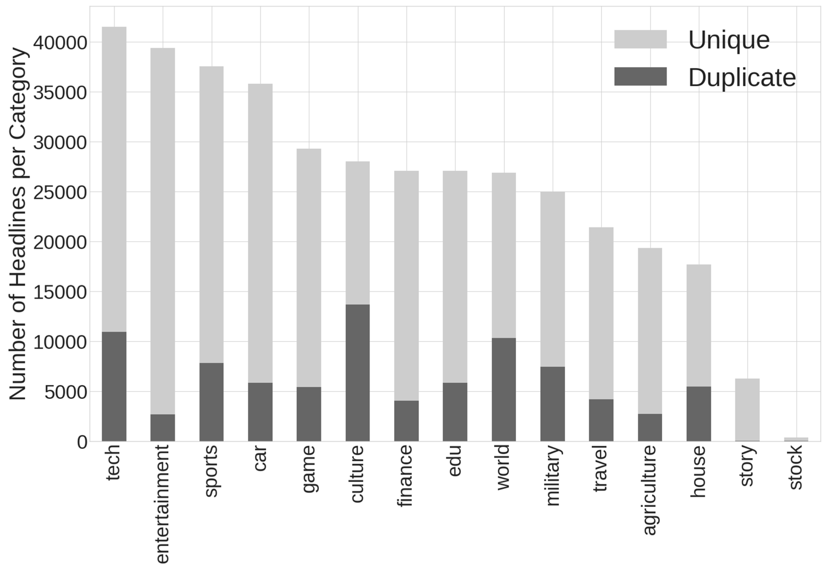
Because this dataset was from an aggregator and it was possible the site captured the same article from multiple sources, a search for duplicate headlines was conducted. The result of this search is displayed in
Figure 1, which is a countplot generated from the 15 topic categories and gives insight into a flaw in the dataset—an excessive number of duplicate entries in certain categories. There are a total of 86,195 duplications (22.5% of the dataset), which can cause an inaccurate calculation of model metrics and result in models inappropriately focusing more on high-duplicate categories such as culture.
Figure 1 also highlights a class imbalance, especially for the story and stock categories.
1.2. Literature
In the literature, many researchers have applied various methods and strategies to the NLP of Chinese text, and some of these have used the Toutiao dataset.
Table 2 gives a summary of prior work using the Toutiao dataset along with the method, metrics, complexity of each model, and the corresponding results. As with all data analytics techniques, the details of how each methodology is configured are incredibly important and, in some cases, very complex. One noteworthy aspect identified in the literature search is in the rightmost column—none of the prior work removed duplicate headlines. Analyses of other Chinese short-text datasets are present in the literature, with Xu et al. describing the performance of a variety of algorithms on four datasets, achieving 72–99% accuracy [
5].
The concept of pre-trained language models such as BERT and ERNIE have proven effective for improving the performances of various natural language understanding and generation tasks [
6,
7]. Pre-trained language models are generally trained on a large amount of text data in a self-supervised manner and then fine-tuned on downstream tasks or directly deployed through zero-shot learning without task-specific fine-tuning. BERT is a pre-trained model that has demonstrated high performance and is appropriate for text classification (our case), named entity recognition, and sentiment analysis [
8]. This architecture differs from decoder-based models such as GPT and sequence-to-sequence models that include Pegasus [
9] and BART [
10]. For comparable work in English, similar work by De Pietro compared three different NLP methods and showed a general accuracy at a minimum of 84% for classifying English headlines and higher accuracies on some models focusing on three classification categories [
11]. This paper will attempt to reach a general minimum accuracy of 0.80 across 14 categories, which is a lower accuracy when compared with De Pietro, but analyzes a different dataset with a broader number of categories. Another goal of this paper is to analyze the tradeoffs between model performance, model complexity, and prediction speed.
Table 2.
Summary of literature analyzing the Toutiao dataset.
Table 2.
Summary of literature analyzing the Toutiao dataset.
| Source | Methodology | Measure of Goodness | Complexity | Pre-Training Used | Notes |
|---|
| [12] | Combined neural topic model (ProdLDA) with a Convolutional NN | 85% Accuracy
85% Precision
85% Recall
85% F1 Score | Seven-step method to prepare/extract features | None | N = 382,688
Duplicates
retained |
| [13] | Feature-enhanced non-equilibrium bi-directional long short-term memory (NE-BiLSTM) NN | 91.71% Precision
91.66% Recall
91.68 F1 Score | Three Components- -
BERT+ - -
Nebi-LSTM - -
Hierarchical Attention Model
| BERT
word vector training method | N = 300,000
Duplicates
retained |
| [14] | Hypernetwork-based architecture to model the descriptive meta-information and integrate it into pre-trained language models with LSTM NN | 90.05% Accuracy | Three Components- -
Pre-trained Model Encoder - -
Hyper Encoding (LSTM) - -
Infer Encoding (LSTM)
| RoBERTa | N = 382,688
Duplicates
retained |
| [15] | Multi-kernel convolution NN with label-oriented attention mechanism | 86% Accuracy
85% Precision
87% Recall
86% F1 Score | Five Components- -
extract text feature information - -
aggregate the information of the token features - -
generate sentence vector - -
generate final sentence representation - -
predict final label
| None | N = 382,688
Duplicates
retained |
| [16] | Fusion of BERT-based model, semantic features, and Bidirectional Gate Recurrent Unit (BiGRU) | 87% Accuracy | Three Components- -
TF-IDF weighting - -
Semantic input from BiGRU CNN - -
Fusion of semantic and statistical feature
| BERT | N = 70,000
Duplicates
retained |
| [17] | BiLSTM and TextCNN, followed by fully-connected layers | 89.9% F1 Score | Three Components- -
BiLSTM - -
TextCNN - -
Fusion of two inputs
| ERNIE | N = 221,000
Duplicates
retained |
| [18] | Single Layer Convolutional NN using pixel glyphs | 87% Accuracy | Three-Step Method- -
convert Chinese text to glyph pixel matrix - -
extract forward and backward n-gram features - -
apply 1-dim max-over-time pooling
| None | N = 382,688
Duplicates
retained |
| Present work | Several algorithms | Refer to
Section 3 | - -
Naïve Bayes - -
XGBClassifier - -
Sequential NN - -
BERT
| Evaluate five options | N = 382,688
86,195
duplicates
removed |
2. Materials and Methods
The code for the models was prepared and executed within a Python 3.10.12 environment using sklearn 1.2.2 and keras 2.14.0. A 16 GB NVIDIA T4 Tensor Core GPU was used, and the CRISP-DM process was followed, with the phases of data understanding, data preparation, modeling, and evaluation [
19]. The methods described below primarily use these libraries for the models and for the preparation of the text, with the assistance of numpy, pandas, and other common multi-task Python libraries. Many NLP libraries such as NLTK, spaCy, and word2vec were not used as they were created for Western languages; applying them to non-Western languages can lead to unintended results. An additional library used for the paper was the jieba library, which was created to segment Chinese text into “words” for NLP tasks due to the Chinese language’s lack of space separation in writing [
20]. The BERT Chinese-language tokenizer
bert-base-chinese was used in the BERT models.
Four algorithms were evaluated for their performance on this dataset: Naïve Bayes, XGBClassifier, BERT, and neural network (sequential). For the first three approaches, an 85%/15% train/holdout split was used to monitor overfitting since there are many data points available. For the NN-sequential approach, a 70%/15%/15% train/validate/holdout split was used where the model is trained with the train set, the validation set is used for making decisions about hyperparameters, and the test set is used to evaluate a few selected models with the best performance. A stratified split is used to make sure minority classes are represented due to the class imbalance noted in
Figure 1.
Other methods described below include the NLP processing techniques used, the six iterations of data preparation that were evaluated in this work, and details related to the four families of algorithms that were applied to this dataset.
2.1. Natural Language Processing
Simplified Chinese Mandarin characters dominated the dataset, with only a small number of headlines in traditional characters. In Chinese Mandarin, the meanings of traditional and simplified characters are generally the same, so training only needs to happen on one character set if the traditional characters are converted to simplified. Written dialects of Chinese, such as Cantonese, were not in the dataset and, therefore, were not considered in this study.
Initial data processing created the stop words list and segmented the headlines [
21]. In NLP, stop words are words, characters, or symbols in a text that typically convey little meaning but may perform a grammar function or other purpose and that are generally considered unimportant when labeling the data [
21,
22]. Stop words tend to rise toward the top of frequency lists of words as they are often the most common elements of a corpus and are removed from a text before it is processed by a model. Stop word removal was part of the pre-processing for each model. A custom-built set of 83 stop words was determined by examining the frequencies of characters and words in the training set. The stop word list contained English words such as the/and/is, individual Chinese characters, Chinese “words” created from the jieba encoder, and common punctuation marks. All algorithms used this stop word list except for BERT, which did not use stop words. As a transformer model, BERT derives context from the surrounding words, and excluding stop words could hurt performance. After an analysis of the frequencies of characters and words in the training set, candidate stop words were selected and written in a text file.
The 382,688-entry dataset contained both English and Chinese, and the number of English-only headlines was found to be minuscule—all categories had 2 or fewer English-only headlines except for one 36-count category. As a result, headlines with English words were retained. Stemming and lemmatization are common NLP steps that deconstruct a word to arrive at the shared meaning in similarly spelled words since it is the meaning that should be modeled with the other words in the text. Stemming is a relatively simple process that truncates the end of a word; for example, process, processed, and processing would all be reduced to process. Lemmatization is a more complex process that addresses plurals, tenses, and gerunds in order to reduce the word to its base form, also known as a lemma. Chinese does not have these elements, so stemming and lemmatization were not required [
21].
The vocabulary provided to the models, also known as the set of unique tokens, was evaluated by character-level and word-level approaches. The character-level vocabulary had a size of 5888 characters. It represented all of the characters used throughout the headline corpus and could be used because of the way each Chinese character retains a meaning that is often similar, regardless of the surrounding characters. After applying jieba to the training corpus, the word-level vocabulary had 167,506 words. Limiting the size and selection of these vocabularies provided an option for tuning the models, and models were built ranging from 25 words in increments to the maximum vocabulary [
11]. Vectorization and feature selection occurred via
sklearn Count Vectorizer for bag-of-words (word count) encoding,
sklearn TF-IDF for statistical TF-IDF encoding,
keras TextVectorization for NN TF-IDF encoding, and BertTokenizer for the BERT models. The NLP processing steps varied per algorithm, and a summary is provided in
Table 3. More details on each algorithm are provided in
Section 2.3.
2.2. Data Preparation Investigations
In this work the resulting model performance from a variety of data preparation steps are evaluated, which are labeled variations A/B/C/D/E. The individual influence of these data preparation steps are studied, and then the steps that contribute positively to model performance are combined as variation F.
Baseline: The baseline dataset has duplicate entries removed but no other adjustments. After removing 86,195 duplicates, there are 296,493 entries in 15 categories. Headlines with mixtures of Chinese text and non-Chinese text were retained, as were 44 English-only headlines. All other variations (B–F below) start with this dataset.
Remove stock category: As shown in
Figure 1, the stock category of news headlines was vastly underrepresented when compared to the other categories. This version of the dataset removed this category.
Remove whitespace: This version removed any whitespace at the beginning or end of the headline.
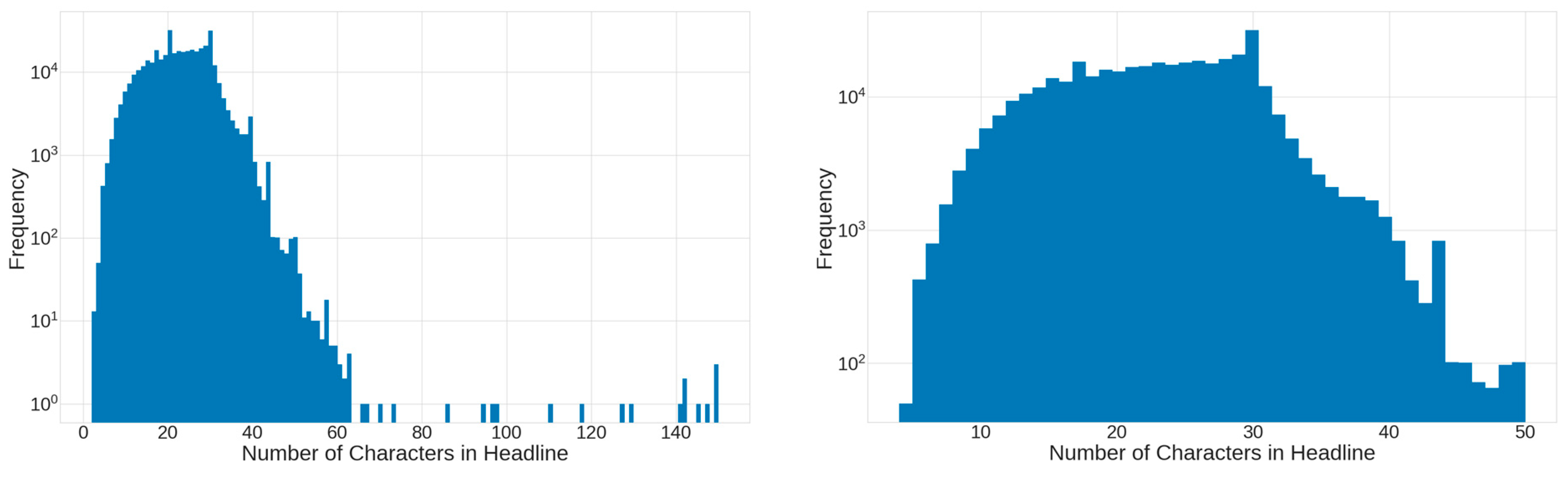
Standardize headline length: The lengths of the headlines were examined, and they varied from 2 to 150 characters in length. The median headline length was 23 characters, with the smallest median of 18 for the culture category and the longest of 28 for the story category. A plot of frequency vs. headline characters is shown in
Figure 2. The left side of the figure shows a countplot of the number of characters in all headlines. This variation was adjusted by removing headlines that exceeded 50 characters in length or were shorter than 3 characters. The right side of
Figure 2 shows the countplot after these headlines are removed.
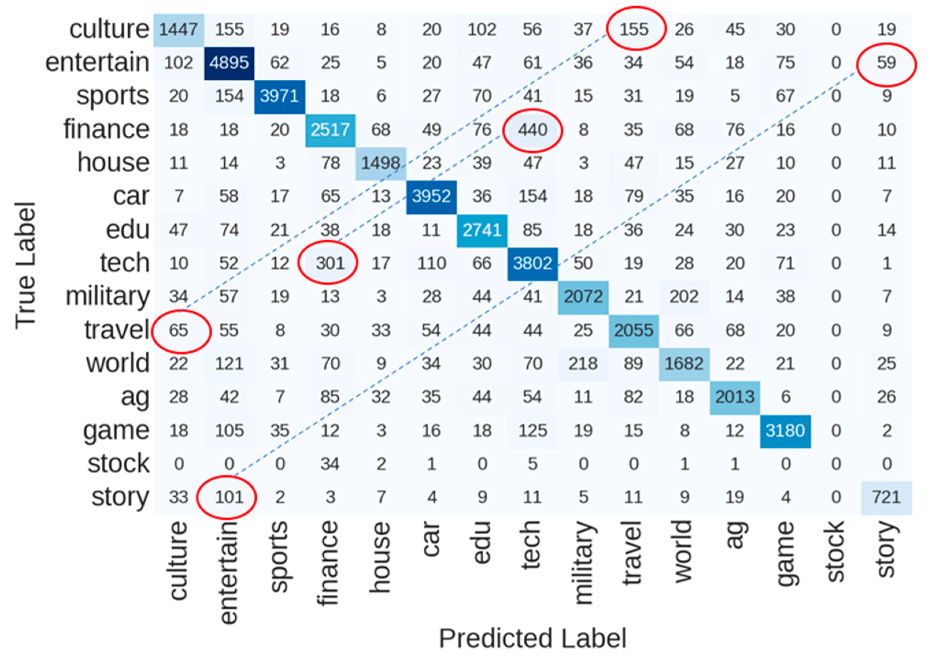
Combine similar categories: The confusion matrix from a baseline (version A) model is presented in
Figure 3, which shows common errors between pairs of categories. While every pair of categories has some degree of error, these 3 were selected to investigate this technique as the authors believed there was a logical connection between them: finance and tech, culture and travel, and entertainment and story.
Best: Detailed modeling and analysis showed that, on average, the algorithms benefited most from data preparation approaches that removed the under-represented stock category (variation B), did not remove whitespace at the beginning/end of a headline (variation C), did not standardize the headline length to 3–50 characters (variation D), and combined 3 pairs of related categories (variation E).
2.3. Metrics and Algorithms
A multi-class classification attempts to discern which single label to apply to the data. In this study the accuracy averaged across all classes was selected as the primary metric, as the penalty for an incorrect prediction was equal across the classes. Accuracy is the overall effectiveness represented by the sum of true positives and true negatives divided by the total sum of results and was selected as the main performance metric [
23,
24,
25]. This also facilitates a comparison to the literature, as a majority of those papers use accuracy. Other metrics that were evaluated on a case-by-case basis were f1, AUC, precision, and recall. AUC was selected as a metric as sensitivity versus specificity can be easily plotted to provide a visual comparison both for the model as well as for each category [
26]. Precision is the ratio of true positives to true positives plus false positives. Recall is also known as sensitivity and is calculated as the number of true positives divided by the number of true positives and false negatives.
2.3.1. Statistical Model—Multinomial Naïve Bayes
The Multinomial Naïve Bayes scheme was selected as the first modeling algorithm to determine if a simple architecture could perform as well as more complex models, which included pre-training techniques. In the literature, a multinomial Naïve Bayes classifier was paired with a term frequency-inverse document frequency (TF-IDF) vectorizer to achieve 91% accuracy on a different Chinese short-text dataset [
27].
As shown in
Table 3, tokenizing and other functions were incorporated into the natural language processing for this algorithm. As part of the tokenizing and vectorizing process for the Multinomial Naïve Bayes model, word-count vectorization and TF-IDF vectorization techniques were explored [
11,
28,
29]. The
sklearn CountVectorizer module used a bag-of-words approach based on the frequency of each word, or the
sklearn TfidfVectorizer module applied to weight each token against its frequency in the training set. After the chosen vectorization was applied, the stop words were removed from the vocabulary, and the training vocabulary was tokenized and vectorized. After processing, 5888 characters were tokenized at the character level, and 167,506 words were tokenized at the word level. TF-IDF and count-based feature selection were applied to explore a range of 25–5888 characters and 25–167,506 words. The vocabulary sweep was repeated for unigram token selection, uni-/bigram selection, and uni-/bi-/trigram selection.
In Naïve Bayes, token order does not matter, which is part of the naïve quality of the method. From the training set, tokens were assessed for the probability of occurring alongside other tokens within a headline. The relational probabilities were also calculated for every token in their vocabulary. Into this trained model, validation headlines could be inputted, and from the relationships of the tokens, a probability was calculated on how the words in each validation headline were likely to belong to each of the 15 categories, and the highest probability was the winning result for that headline [
30]. This was applied via sklearn’s MultinomialNB module, to which the TF-IDF training vocabulary was fitted. The validation set, in comparison with the training set, was used to monitor for overfitting and tuning of parameters.
2.3.2. Ensemble Model—XGBClassifier
The Python extreme gradient boosting algorithm XGBClassifier was selected to investigate the performance of an ensemble algorithm. Ensemble methods were not applied in the literature surveyed for this work and can often rival the performance of neural networks [
31,
32]. This algorithm is a member of the extreme gradient boosting family, which is an ensemble learning method that combines the predictions of multiple decision trees (boosting) to create a strong predictive model. The decision trees are trained sequentially, and each subsequent tree minimizes the errors made by the prior tree.
Within the XGBClassifier algorithm, the pruning parameter max_depth = 6 was specified to limited overfitting, after exploring a range of max_depth values. Similar to the Naïve Bayes algorithm procedure, TF-IDF and count-based feature selection was applied to explore a range of 25–5888 characters and 25–167,506 words, for unigram, uni-/bigram, and uni-/bi-/trigram token selection methods.
2.3.3. Sequential Neural Network
In this approach, keras neural network models were created using a sequential architecture, and used similar processing functions as the prior algorithms to prepare the data. For word-level neural networks, the data were tokenized by jieba, stop words were removed from the text, and whitespace was inserted between the tokens. These inputs were incorporated into the neural network via a
keras TextVectorization layer, which used the TF-IDF method for feature selection. The TextVectorization layer was also used to examine character-based and word-based tokenization approaches. This was the first layer of the network and was fed into an embedding layer for dimension reduction. A rule of thumb suggested an embedding dimension approximately equal to the fourth root of the vocabulary [
33]. This was calculated as 8 dimensions for the 5888-token vocabulary character-level models and 20 dimensions for the 167,506-token word-level models. For the word-level models, the maximum tokens were limited to 20,000 as it is rare that performance increases can be identified beyond that level [
34] and to avoid memory crashes. To change the dimensions of the embedding layer in preparation for the Dense layers, a Flatten layer was used. A Global Average Pooling 1D layer was investigated as a substitute for the Flatten layer but did not alter performance.
Stochastic gradient descent (SGD) and adaptive moment estimation (Adam) were investigated as optimizer options, and each Dense layer used the ReLU activation function for its neurons. Because each headline was selected into one of many categories, the sparse categorical cross-entropy loss function was used, which penalizes the model when it estimates the incorrect category [
26]. To prevent overfitting, L2 regularization was used at a fixed value of 0.001, and a range of dropout levels was investigated. Overfitting is monitored through the accuracy of the training and validation datasets at each epoch of training—it is known that overfitting occurs when the accuracy of the validation set plateaus while the training set accuracy continues to increase.
To aid in training, a callback was established to halve the learning rate every 15 epochs, and early stopping was used with a patience level of 10 epochs. The Widrow recommendation for the number of neurons is related to the number of data points P = 296,493 non-duplicate entries, the number of weights (neurons × (inputs + 1)), and the desired error level according to Equation (1) below [
35].
According to the Widrow recommendation, for the approximate 10% error level in this work, 30 embedded dimensions are used as inputs and 15 outputs, and the recommendation is a maximum of 63 neurons. In the hyperparameter tuning process, the neuron count was limited to within an order of magnitude of this recommendation.
Within Python, the Adaptive Experimentation Platform (Ax) library was installed and used to tune the neural network model’s hyperparameters. The training dataset was split into training and validation, and the hyperparameters were tuned using the validation dataset. After tuning, the final model performance was calculated using the test/holdout dataset. Bayesian optimization was used for numeric features, except for the categorical optimizer feature, where Bandit optimization was used. Further optimization information is given in
Section 3.3.
2.3.4. BERT Neural Network
A Bidirectional Encoder Representation from Transformers (BERT) model instance from Hugging Face was fine-tuned on the dataset [
36]. This encoder-based model was from the
BERTforSequenceClassification family, and the number of inputs was specified based on the number of labels in the dataset. The dataset was split into 80% train and 20% holdout sections, stratified amongst the labels. To minimize RAM usage, a DataLoader was used with a maximum batch size of 128, and shuffle = True. The
bert-base-chinese tokenizer was trained on the dataset, and the neural networks were trained using TensorFlow and PyTorch. A decoupled weight decay regularization optimizer (AdamW) was specified [
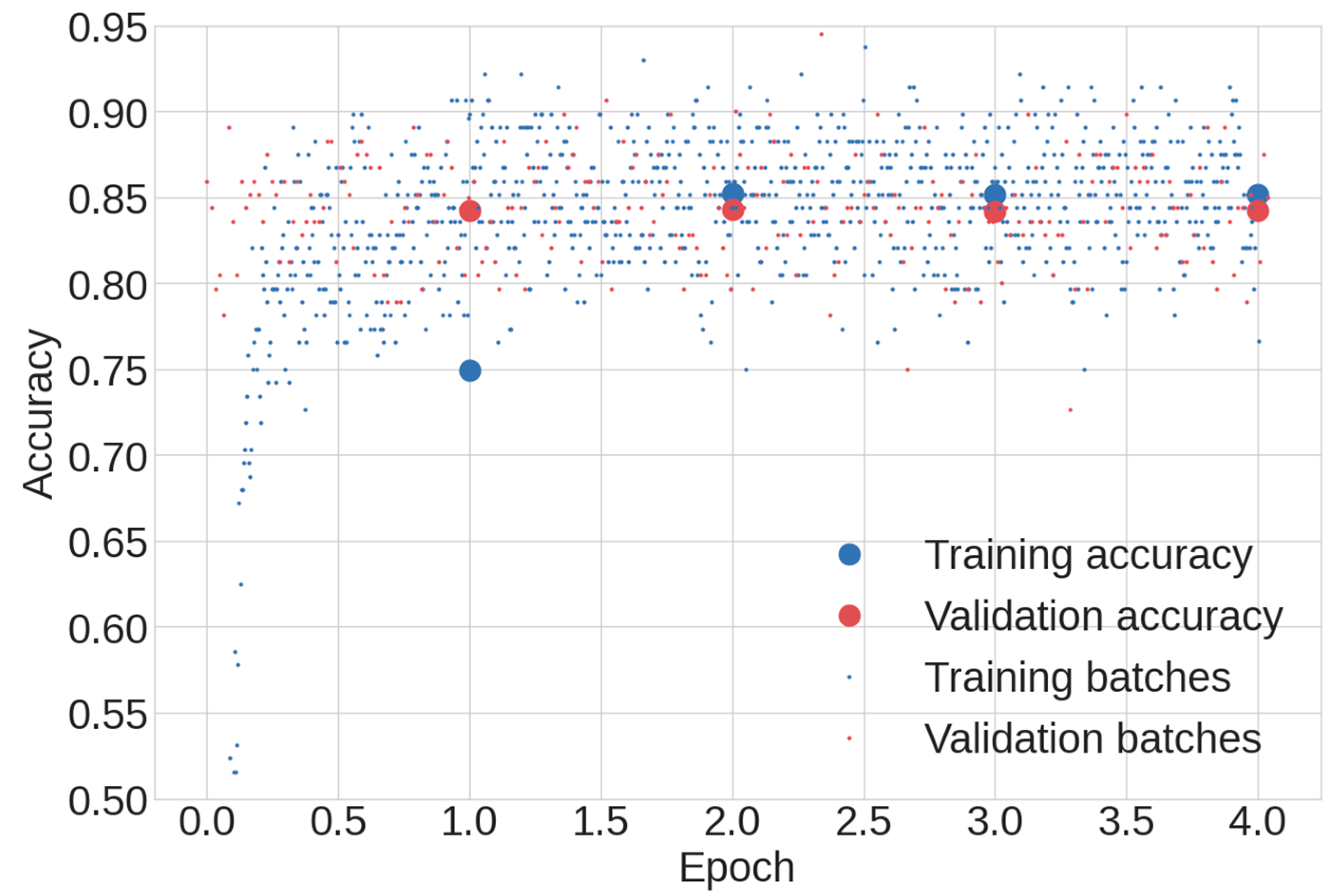
37], and multiclass accuracy was calculated on the training and validation datasets to monitor for overfitting. The training process was lengthy, and both the epoch-level accuracy and batch-level accuracy for a BERT training run are shown in
Figure 4. As shown in the figure, it was common for the accuracies to stabilize at 2 epochs, so that was selected as the epoch hyperparameter. A limited hyperparameter sweep of learning rates and batch sizes was conducted to find that the best performance resulted in a learning rate of 2 × 10
−5 and a batch size of 32. With the low batch size, each 2-epoch training run took approximately 3 hours.
3. Results
In this section, the performance of four machine learning algorithms is evaluated on datasets with dataset versions A–F. A summary of the main hyperparameter settings and model performance is presented in
Table 4, followed by detailed results for each algorithm. Based on the exploration in this work, performances are given for the best set of encoding and hyperparameters for each algorithm, which are indicated in the notes column. As visible in the table, the data preparation steps that made positive contributions (averaged) to the baseline dataset were B and E. These steps were to remove the stock category and combine similar categories, which were used to build dataset version F. In the subsequent sections, modeling results for dataset version A are presented.
3.1. Multinomial Naïve Bayes
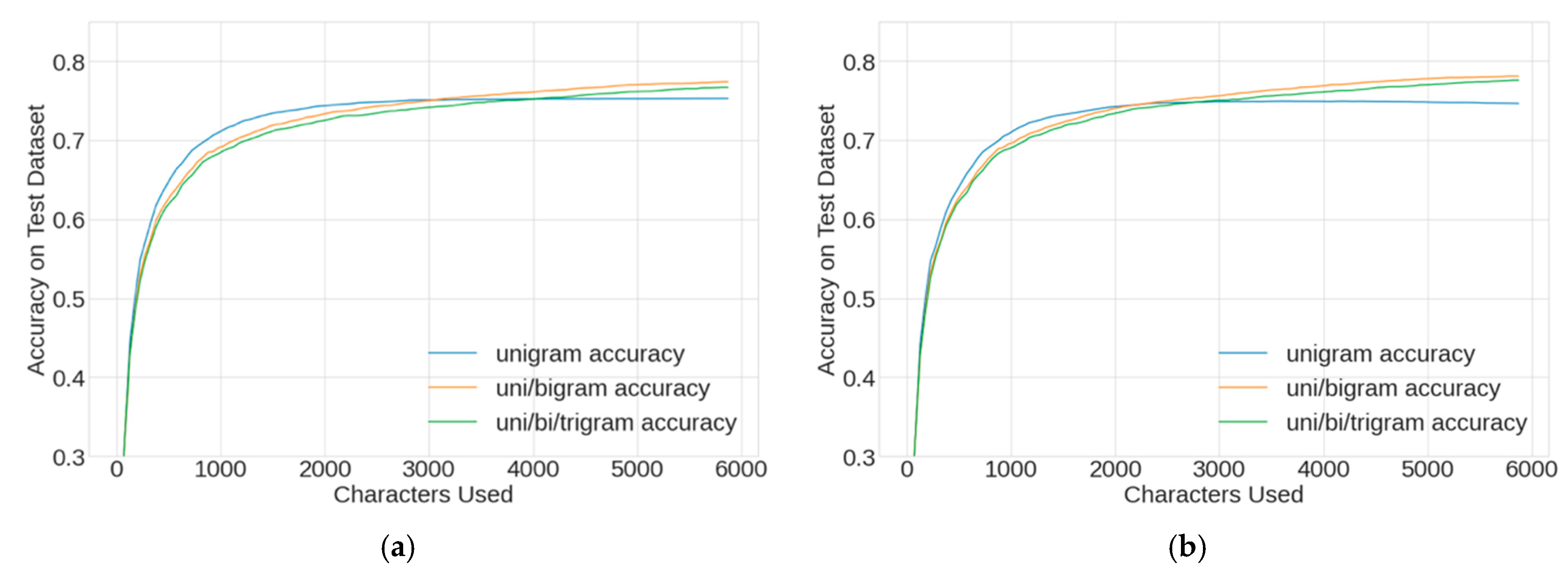
Using dataset version A and character-level tokenization, the results of the hyperparameter sweep on vocabulary and tokenization are presented in
Figure 5. The tokenization approaches included either CountVectorizer or TF-IDF vectorization and explored unigrams, unigrams/bigrams, and unigrams/bigrams/trigrams. The results were similar for CountVectorizer (a) and TF-IDF vectorization (b) methods, where the highest performance was found using the full 5888-token vocabulary. By a small margin, the best character-level model used TF-IDF, unigrams/bigrams, and possessed 78.2% accuracy.
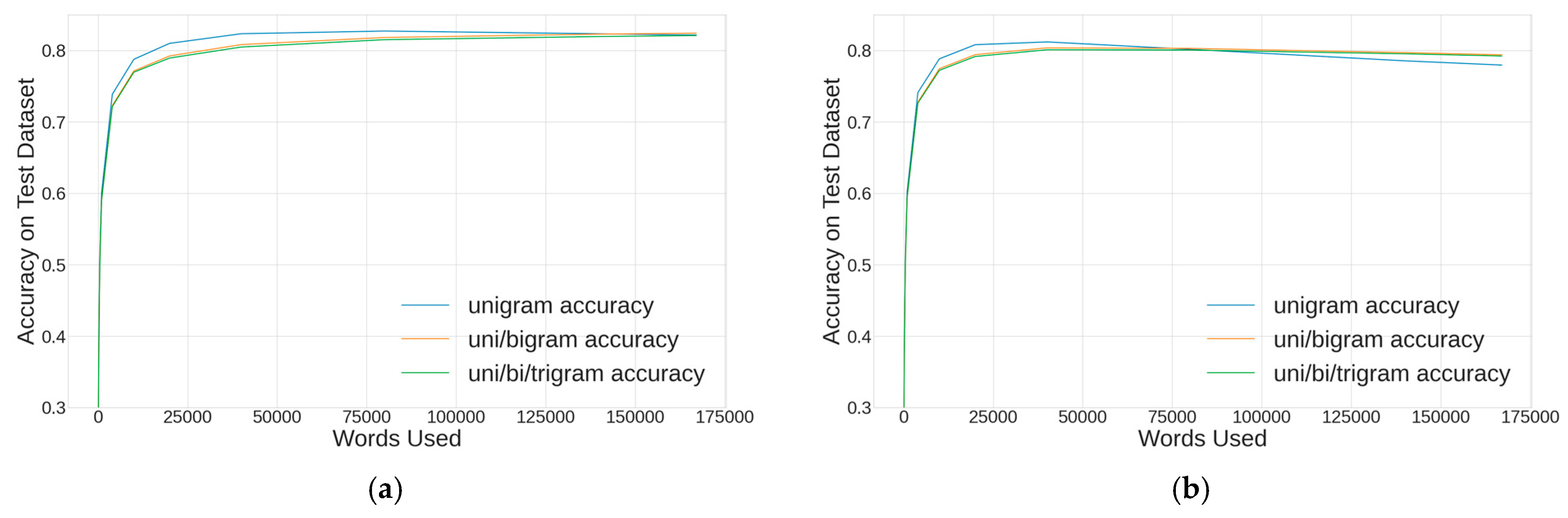
For word-level tokenization, the hyperparameter sweep was repeated and the results are presented in
Figure 6. The approach differed from the character-level tokenization by exploring the full vocabulary of the 167,506 tokens that resulted from applying the jieba method. Again, the results were similar for CountVectorizer (a) and TF-IDF vectorization (b) methods. The best model used the CountVectorizer, unigrams with an 84,025-token vocabulary and possessed 82.8% accuracy.
3.2. XGBClassifier Ensemble Method
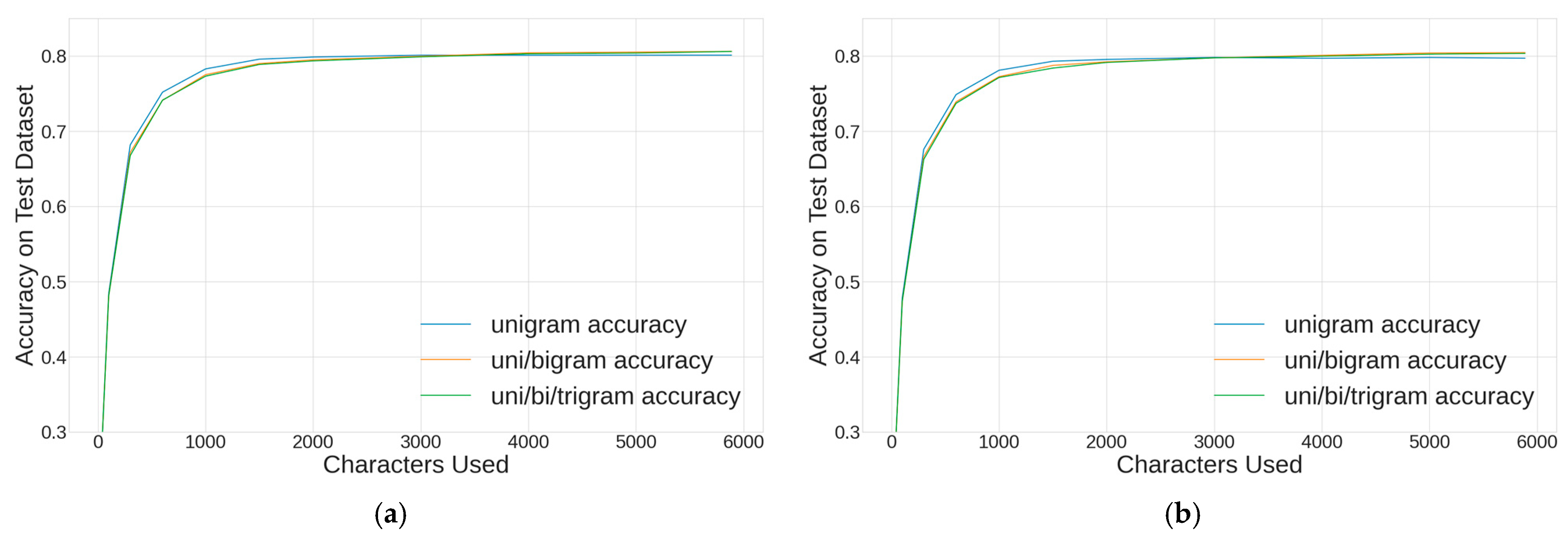
Similar to the Multinomial Naïve Bayes algorithm, a sweep of vocabulary and tokenization was conducted using the ensemble XGBClassifier algorithm.
Figure 7 shows the results for the character-level modeling; the results were similar for CountVectorizer (a) and TF-IDF vectorization (b) methods. The performance plateaued near 2000 tokens, and the best character-level model used the full 5888-token vocabulary. This model used the CountVectorizer, unigrams/bigrams and achieved 81.0% accuracy.
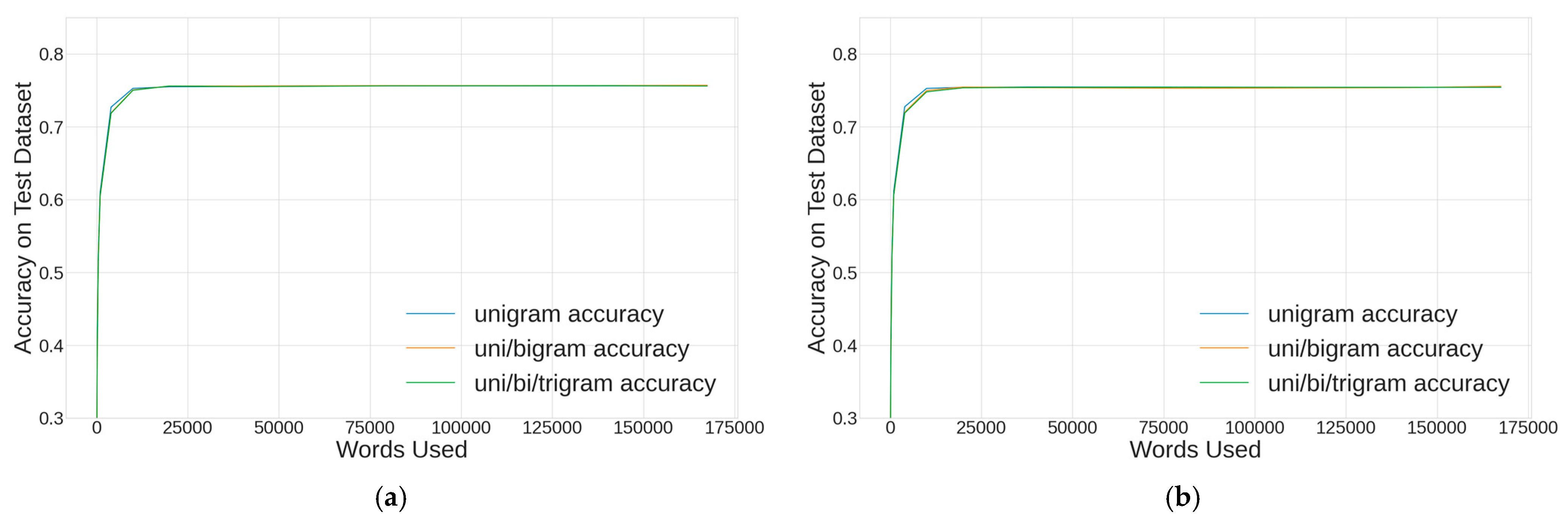
The hyperparameter sweep was repeated for word-level tokenization, where the only change was exploring the full vocabulary of the 167,506 tokens that resulted from the jieba method.
Figure 8 shows that this method did not perform as well for either the CountVectorizer (a) and TF-IDF vectorization (b) methods. The best word-level XGBClassifier model used the CountVectorizer, unigrams, and the full 167,506-token vocabulary and achieved 76.2% accuracy.
3.3. Sequential Neural Network
The Adaptive Experimentation Platform (Ax) library was used to tune the neural network model’s hyperparameters, and Ax converged on a solution after 30 optimization loops.
Table 5 presents a summary of the multi-dimensional hyperparameter tuning using Ax, including the hyperparameters tuned, their search range, the best set of hyperparameters for the character-level and word-level approaches, and the performance achieved on the holdout dataset. These sets of hyperparameters were used to create sequential neural network models for data preparation versions A–F.
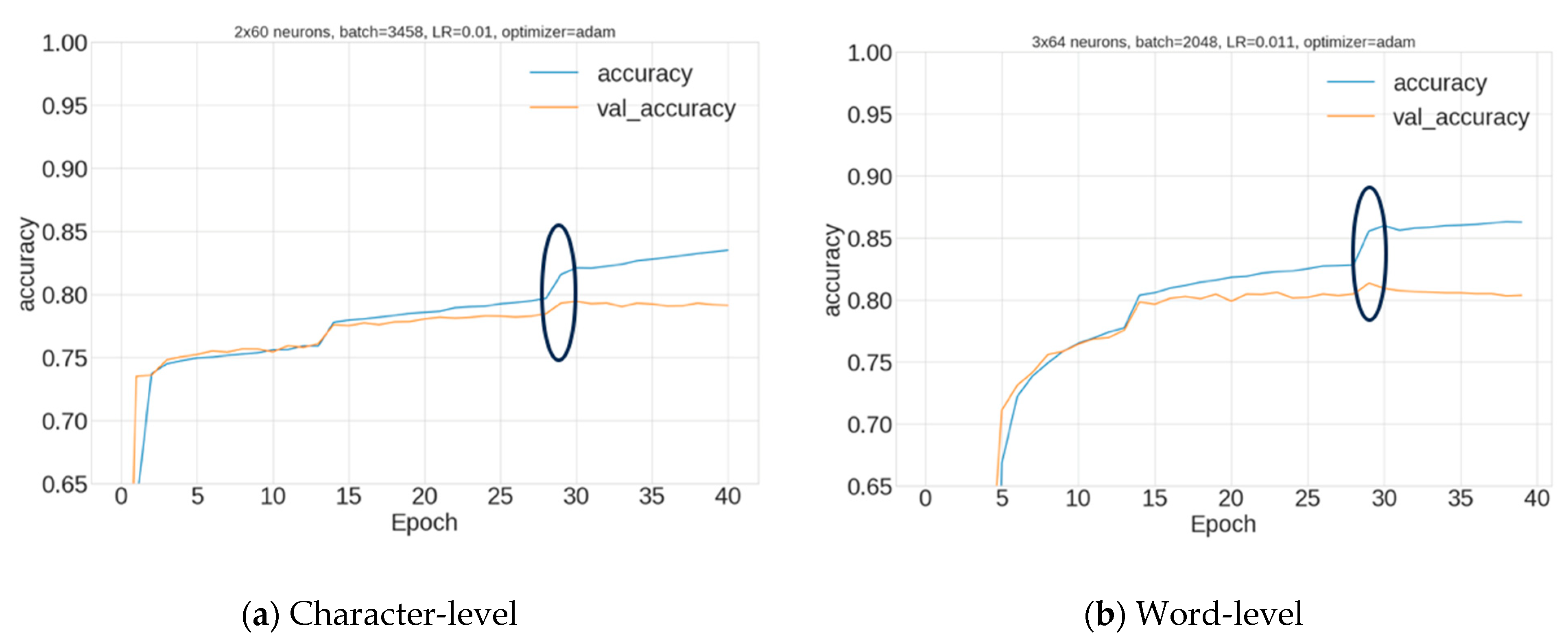
Models were saved during optimization, and the best model’s train/validation curves are shown in
Figure 9 for the best character-level (a) and word-level (b) models. Both sets of curves show the model is exhibiting normal training behavior. The impact of the decreasing learning rate is visible in
Figure 9, which halves every 15 epochs of training and enables a small boost in performance at 15 and 30 epochs. Also, the early stopping callback allowed the model to be saved at the highest validation performance, which is denoted by the black oval. This enables the model to avoid higher levels of overfitting.
3.4. BERT Neural Network Modeling
The highest performance was achieved using the BERT transformer models, using the results of the exploration that identified the optimal set of hyperparameters as epochs = 2, learning rate = 2 × 10
−5, and batch size = 32. The best-in-class model used data-preparation steps that removed the under-represented stock category (B), combined three pairs of related categories (D), did not remove whitespace at the beginning/end of a headline, and did not standardize the headline length to 3–50 characters. The detailed metrics for this model are presented in
Section 4.
4. Discussion
From examining
Table 4, it can be seen that there are two notable high-performing models on this dataset from the simplest and most complex algorithms tested. The simplest algorithm (Naïve Bayes using dataset variation F) achieved 85.1% accuracy on the test dataset, using a jieba word-level CountVectorizer with 84,025 unicode tokens. This model size was 15 MB, does not require a GPU, took a total of 45 s to train the vectorizer, and the model can predict 3,625,000 headlines per second. The most complex algorithm (NN BERT) achieved 89.3% accuracy using the hyperparameters of 2 × 10
−5 learning rate, batch size of 32, and 2 epochs of training. The model size was 409 MB, and training the vectorizer and model took 2.1 hours with an NVIDIA T4 GPU. The model could predict 195 headlines per second.
There are vast differences in time and computing resources between the two best algorithms, as the BERT model required 170× more time to train, was slower to predict by a factor of 18,600, and required 27× more disk space to save the model. This model could be the best choice for a low-volume application when the highest accuracy is needed. For applications on a larger scale where a slight degradation in performance can be tolerated, the Naïve Bayes algorithm could be the best choice.
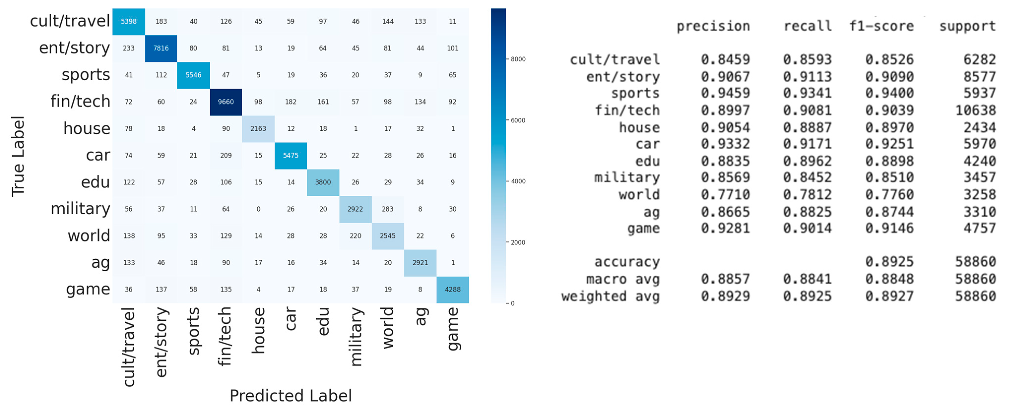
The detailed model performance of the tuned BERT algorithm is presented in
Figure 10, with the confusion matrix on the left and the classification report on the right. The model performed fairly consistently on the test/holdout dataset across all categories, with the exception of the world category, which possessed F1 = 77.6%. On the left side of the figure, the model had the highest level of confusion between the military and world categories and between the finance/technology and car categories.
Considering the high volume of Chinese language articles posted online on any given day that a typical Chinese researcher needs to process, deploying this model in a web scraper could assist in the initial selection of articles for analysis.
Web scrapers are easy to build and deploy and are commonly used by researchers and journalists to automate the collection of news articles from online sources. They are cheap and effective to use but often use exact keyword matching to select articles for retention. Keyword matching can grab unintended articles and miss articles of interest. Keyword lists also require maintenance to keep up with changes in keywords. Applying the models developed in this work would reduce the number of extraneous articles collected, increase the collection of articles of interest, and eliminate the need to maintain keyword lists. This would result in overall savings by allowing the web scraper to complete its task more efficiently and in less time and enabling researchers to focus on the most relevant articles. This method could also reduce computer memory storage requirements as it selects a higher number of relevant articles and fewer unnecessary articles. It would also enable researchers who are not language-enabled to effectively use the scraper, allowing language-enabled researchers to focus efforts elsewhere.
5. Conclusions
Given the volume and scope of Chinese-based language articles generated each day and the limited amount of time and personnel to review the material, it is a true challenge to effectively find and analyze relevant works. It is, therefore, essential to reduce the number of candidate articles for review. Efficient and, perhaps more importantly, accurate categorization of news articles is the first step toward this goal. Using automated processes offers increased capability if the methods used can be trusted and are accomplished in a timely manner. This paper explored combining natural language processing with machine learning to solve this problem.
Specifically, several data preprocessing methods based on NLP methods were used to pre-process Chinese-language news articles for use in four machine-learning algorithms, resulting in the classification of those articles into 15 general topic categories. The results show that the accuracy of the methods involved approached 90% and were robust enough to be applied in a live setting to obtain useful results. However, it was also discovered that model complexity significantly impacted processing time and storage requirements, thus indicating that the usefulness of each method may be dependent on the time and accuracy constraints required by the user. Also, 22.5% of the Toutiao dataset consists of duplicate records, and this work is the first published analysis with duplicates removed. As such, it sets a new benchmark for comparison to future work even though its model performance does not exceed those found in the literature.
Author Contributions
Conceptualization, D.G. and T.W.; methodology, D.G., T.W. and B.L.; software, D.G. and T.W.; validation, D.G. and T.W.; formal analysis, D.G. and T.W.; investigation, D.G.; resources, T.W.; data curation, D.G.; writing—original draft preparation, D.G., T.W. and B.L.; writing—review and editing, T.W. and B.L.; visualization, D.G. and T.W.; supervision, T.W. and B.L.; project administration, T.W. and B.L. All authors have read and agreed to the published version of the manuscript.
Funding
This research received no external funding.
Data Availability Statement
The dataset is publicly available [
4].
Conflicts of Interest
The authors declare no conflicts of interest.
Authors’ Note
The views expressed are those of the authors and do not reflect the official guidance or position of the United States Government, the Department of Defense, the United States Air Force, the United States Space Force or any agency thereof. Reference to specific commercial products does not constitute or imply its endorsement, recommendation, or favoring by the U.S. Government. The authors declare this is a work of the U.S. Government and is not subject to copyright protections in the United States. This article has been cleared with case numbers 88ABW-2023-1067 and MSC/PA-2023-0204.
References
- Policy Planning Staff. The Elements of the China Challenge; U.S. Secretary of State: Washington, DC, USA, 2020. [Google Scholar]
- Williams, H.J.; Blum, I. Defining Second Generation Open Source Intelligence (OSINT) for the Defense Enterprise. 2018. Available online: https://www.rand.org/pubs/research_reports/RR1964.html (accessed on 1 August 2022).
- Li, J.; Wang, B.; Ni, A.J.; Liu, Q. Text Mining Analysis on Users’ Reviews for News Aggregator Toutiao. In Proceedings of the International Conference on Artificial Intelligence in Information and Communication, Fukuoka, Japan, 19–21 February 2020. [Google Scholar]
- Github User Aceimnorstuvwxz. Github User Aceimnorstuvwxz. Github Toutiao Text Classfication Dataset (Public). July 2018. Available online: https://github.com/aceimnorstuvwxz/toutiao-text-classfication-dataset (accessed on 21 July 2022).
- Xu, Q.; Peng, J.; Zheng, C.; Tan, S.; Yi, F.; Cheng, F. Short Text Classification of Chinese with Label Information Assisting. ACM Trans. Asian Low-Resour. Lang. Inf. Process. 2023, 22, 1–19. [Google Scholar] [CrossRef]
- Xu, L.; Hu, H.; Xhang, X.; Li, L.; Cao, C.; Lan, Z. CLUE: A Chinese Language Understanding Evaluation Benchmark. arXiv 2020, arXiv:2004.05986. [Google Scholar]
- Wang, S.; Sun, Y.; Xiang, Y.; Wu, Z.; Ding, S.; Gong, W.; Wang, H. Ernie 3.0 titan: Exploring larger-scale knowledge enhanced pre-training for language understanding and generation. arXiv 2021, arXiv:2112.12731. [Google Scholar]
- Zhang, A.; ChatGPT and Other Transformers: How to Select Large Language Model for Your NLP Projects. Medium, 2 2023. Available online: https://alina-li-zhang.medium.com/chatgpt-and-other-transformers-how-to-select-large-language-model-for-your-nlp-projects-908de1a152d8 (accessed on 7 March 2023).
- Zhang, J.; Zhao, Y.; Saleh, M.; Liu, P.J. PEGASUS: Pre-training with Extracted Gap-sentences for Abstractive Summarization. In Proceedings of the 37th International Conference on Machine Learning, Vienna, Austria, 13–18 July 2020. [Google Scholar]
- Lewis, M.; Liu, Y.; Goyal, N.; Ghazvininejad, M.; Mohamed, A.; Levy, O.; Stoyanov, V.; Zettlemoyer, L. BART: Denoising sequence-to-sequence pre-training for natural language generation, translation, and comprehension. In Proceedings of the 58th Annual Meeting of the Association for Computational Linguistics, Online, 5–10 July 2020. [Google Scholar]
- Di Pietro, M. Text Classification with NLP: Tf-Idf vs. Word2Vec vs. BERT. Toward Data SCience, 18 July 2020. Available online: https://towardsdatascience.com/text-classification-with-nlp-tf-idf-vs-word2vec-vs-bert-41ff868d1794 (accessed on 2 August 2022).
- Ge, J.; Lin, S.; Fang, Y. A Text Classification Algorithm Based on Topic Model and Convolutional Nueral Network. J. Phys. Conf. Ser. 2021, 1748, 032036. [Google Scholar] [CrossRef]
- Huan, H.; Yan, J.; Xie, Y.; Chen, Y.; Li, P.; Xhu, R. Feature Enhanced Non-Equilibrium Bi-Directional Long Short-Term Memory Model for Chinese Text Classification. IEEE Access 2020, 8, 199629–199637. [Google Scholar] [CrossRef]
- Duan, W.; He, X.; Zhou, Z.; Rao, H.; Thiele, L. Injecting Descriptive Meta-Information Into Pre-trained Language Models with Hypernetworks. In Proceedings of the Interspeech, Brno, Czechia, 30 August–3 September 2021. [Google Scholar]
- Xia, F. Laebl Oriented Hierarchical Attention Neural Network for Short Text Classification. Acad. J. Eng. Technol. Sci. 2022, 5, 53–62. [Google Scholar]
- Luo, X.; Yu, Z.; Zhao, Z.; Zhao, W.; Wang, J.-H. Effective short text classification via the fusion of hybrid features for IoT social data. Digit. Commun. Netw. 2022, 8, 942–954. [Google Scholar] [CrossRef]
- Zhang, M.; Shang, X. Chinese Short Text Classification by ERNIE Based on LTC_Block. Hindawi Wirel. Commun. Mob. Comput. 2023, 2023, 9840836. [Google Scholar] [CrossRef]
- Liu, B.; Lin, G. Chinese Document Classification with Bi-Directional Convolutional Language Model. In Proceedings of the 43rd Internation ACM SIGIR Conference on Research and Development in Information Retrieval, Virtual Event, China, 25–30 July 2020. [Google Scholar]
- IBM Corporation. IBM SPSS Modeler CRISP-DM Guide; IBM Corporation: Armonk, NY, USA, 2011. [Google Scholar]
- Github User fxsjy (Sun Junyi), “fxsjy/jieba,” 15 February 2020. Available online: https://github.com/fxsjy/jieba (accessed on 21 July 2022).
- Kung, S.; Chinese Natural Language (Pre)processing: An Introduction. Towards Data Science, 20 November 2020. Available online: https://towardsdatascience.com/chinese-natural-language-pre-processing-an-introduction-995d16c2705f (accessed on 2 August 2022).
- Deb, N.; Jha, V.; Panjiyar, A.K.; Gupta, R.K. A Comparative Analysis Of News Categorization Using Machine Learning Approaches. Int. J. Sci. Technol. Res. 2020, 9, 2469–2472. [Google Scholar]
- Grandini, M.; Bagli, E.; Visani, G. Metrics for Multi-Class Classification: An Overview. 14 August 2020. Available online: https://arxiv.org/pdf/2008.05756.pdf (accessed on 17 August 2022).
- James, G.; Witten, D.; Hastie, T.; Tibsharani, R. An Introduction to Statistical Learning with Applications in R; Springer: Berlin/Heidelberg, Germany, 2013. [Google Scholar]
- Sokolova, M.; Lapalme, G. A Systematic Analysis of Performance Measures for Classification Tasks. Inf. Process. Manag. 2009, 45, 427–437. [Google Scholar] [CrossRef]
- Géron, A. Hands-on Machine Learning with Scikit-learn, Keras, and TensorFlow; O’Riley: Sebastopol, CA, USA, 2019. [Google Scholar]
- Liu, X.; Wang, S.; Lu, S.; Yin, Z.; Li, X.; Yin, L.; Tian, J.; Zheng, W. Adapting Feature Selection Algorithms for the Classification of Chinese Texts. Systems 2023, 11, 483. [Google Scholar] [CrossRef]
- Das, M.; Kamalanathan, S.; Alphonse, P. A Comparative Study on TF-IDF Feature Weighting Method and its Analysis using Unstructured Dataset. In Proceedings of the COLINS-2021: 5th International Conference on Computational Linguistics and Intelligent Systems, Kharkiv, Ukraine, 22–23 April 2021. [Google Scholar]
- Soma, J. TF-IDF with Chinese Sentences. Data Science for Journalism. Available online: https://investigate.ai/text-analysis/using-tf-idf-with-chinese/ (accessed on 31 August 2022).
- Shishupal, R.S.; Varsha; Mane, S.; Singh, V.; Wasekar, D. Efficient Implementation using Multinomial Naive Bayes for Prediction of Fake Job Profile. Int. J. Adv. Res. Sci. Commun. Technol. 2021, 5, 286–291. [Google Scholar] [CrossRef]
- Saul, J.; Wagner, T.; Mbonimpa, E.; Langhals, B. Atmospheric Meteorological Effects on Forecasting Daily Lightning Occurrence at Cape Canaveral Space Force Station. In Proceedings of the World Congress in Computer Science, Computer Engineering, and Applied Computing, Las Vegas, NV, USA, 24–27 July 2023. [Google Scholar]
- Tucker, T.; Wagner, T.; Auclair, P.; Langhals, B. Machine Learning Prediction of DoD Personal Property Shipment Costs. In Proceedings of the World Congress in Computer Science, Computer Engineering, and Applied Computing, Las Vegas, NV, USA, 24–27 July 2023. [Google Scholar]
- Lakshmanan, V.; Robinson, S.; Munn, M. Machine Learning Design Patterns; O’Reilly Media: Sebastopol, CA, USA, 2020. [Google Scholar]
- Google. Google Machine Learning Course Step 3: Prepare Your Data. 18 July 2022. Available online: https://developers.google.com/machine-learning/guides/text-classification/step-3 (accessed on 22 October 2023).
- Widrow, B. ADALINE and MADALINE. In Proceedings of the 1st International Conference on Neural Networks, San Diego, CA, USA, 23 June 1987. [Google Scholar]
- Devlin, J.; Chang, M.; Lee, K.; Toutanova, K. BERT: Pre-training of deep bidirectional transformers for language understanding. arXiv 2018, arXiv:1810.04805. [Google Scholar]
- Loshchilov, I.; Hutter, F. Decoupled Weight Decay Regularization. In Proceedings of the International Conference on Learning Representations, New Orleans, LA, USA, 6–9 May 2019. [Google Scholar]
Figure 1.
Countplot of all news categories, showing number of unique headlines (light grey) and duplicate headlines (dark grey).
Figure 1.
Countplot of all news categories, showing number of unique headlines (light grey) and duplicate headlines (dark grey).
Figure 2.
Countplot of headlines vs. number of Chinese characters in original dataset (left) and with outliers removed (right).
Figure 2.
Countplot of headlines vs. number of Chinese characters in original dataset (left) and with outliers removed (right).
Figure 3.
Confusion matrix from a model created from version A of the dataset. Similar categories are circled in red, and a dashed blue line designates pairs of categories that were combined in version E of the dataset.
Figure 3.
Confusion matrix from a model created from version A of the dataset. Similar categories are circled in red, and a dashed blue line designates pairs of categories that were combined in version E of the dataset.
Figure 4.
A sample BERT training run where training accuracies are plotted in blue, while validation accuracies are plotted in red. Epoch-level accuracy is denoted by a large circular marker, and batch-level accuracy is denoted by a small circular marker.
Figure 4.
A sample BERT training run where training accuracies are plotted in blue, while validation accuracies are plotted in red. Epoch-level accuracy is denoted by a large circular marker, and batch-level accuracy is denoted by a small circular marker.
Figure 5.
Multinomial Naïve Bayes algorithm: character-level model accuracy vs. character vocabulary for CountVectorizer (a) and TF-IDF vectorizer (b). Using the test dataset, unigram performance is shown in blue, unigram/bigram accuracy in orange, and unigram/bigram/trigram in green.
Figure 5.
Multinomial Naïve Bayes algorithm: character-level model accuracy vs. character vocabulary for CountVectorizer (a) and TF-IDF vectorizer (b). Using the test dataset, unigram performance is shown in blue, unigram/bigram accuracy in orange, and unigram/bigram/trigram in green.
Figure 6.
Multinomial Naïve Bayes algorithm: word-level model accuracy vs. word vocabulary for CountVectorizer (a) and TF-IDF vectorizer (b).
Figure 6.
Multinomial Naïve Bayes algorithm: word-level model accuracy vs. word vocabulary for CountVectorizer (a) and TF-IDF vectorizer (b).
Figure 7.
XGBClassifer algorithm: character-level model accuracy vs. character vocabulary for CountVectorizer (a) and TF-IDF vectorizer (b).
Figure 7.
XGBClassifer algorithm: character-level model accuracy vs. character vocabulary for CountVectorizer (a) and TF-IDF vectorizer (b).
Figure 8.
XGBClassifer algorithm: word-level model accuracy vs. word vocabulary for CountVectorizer (a) and TF-IDF vectorizer (b).
Figure 8.
XGBClassifer algorithm: word-level model accuracy vs. word vocabulary for CountVectorizer (a) and TF-IDF vectorizer (b).
Figure 9.
Training curves for the TF-IDF sequential neural network model for the character-encoded model (a) and the word-encoded model (b). Accuracy was calculated using the training dataset (blue lines) and validation dataset (orange lines).
Figure 9.
Training curves for the TF-IDF sequential neural network model for the character-encoded model (a) and the word-encoded model (b). Accuracy was calculated using the training dataset (blue lines) and validation dataset (orange lines).
Figure 10.
Confusion matrix (left) and classification report (right) calculated on the variation F test/holdout dataset for the tuned BERT algorithm.
Figure 10.
Confusion matrix (left) and classification report (right) calculated on the variation F test/holdout dataset for the tuned BERT algorithm.
Table 1.
Dataset examples.
Table 1.
Dataset examples.
| Category | Headline | Translation * | Notes |
|---|
| military | 美国宣布退出伊核协议, 对中东有何重大影响 | The United States announced its withdrawal from the Iran nuclear agreement, what is the major impact on the Middle East | Normal entry |
| education | Couple reunites with lost son | Couple reunites with lost son | Only English |
| finance | 美元加息的含义和目的是什么? | What is the meaning and purpose of the dollar rate hike? | Duplicate |
| game | Made To Game! iGame联合NVIDIA打造极致游戏体验 | Made To Game! iGame collaborates with NVIDIA to create the ultimate gaming experience | Mix of English and Chinese |
Table 3.
NLP pre-processing steps conducted per algorithm.
Table 3.
NLP pre-processing steps conducted per algorithm.
| Step | Naïve Bayes and XGBClassifier | NN-Sequential | BERT |
|---|
| Segmentation, stemming, and lemmatization | not applicable to Chinese | -- | -- |
Tokenize
(determine vocabulary) | 25–5888 characters or
25–167,506 jieba words
Unigrams,
uni-/bigrams, or
uni-/bi-/trigrams | 25–5888 characters or
25–167,506 jieba words
Unigrams | BertTokenizer
bert-base-chinese |
Vectorize method
(select from vocabulary) | sklearn CountVectorizer for count encoding
sklearn TF-IDF for TF-IDF encoding | Keras TextVectorization layer | BertTokenizer provides
vectors |
| Feature selection | Term frequency (CountVectorizer)
TF-IDF score (TF-IDF) | TF-IDF score | All features used |
| Embedding | None | Keras Embedding layer | Word-piece and token
embedding |
| Stop words | Char: none
Word: custom list | Char: none
Word: custom list | Not used |
Table 4.
Accuracy (%) on the test/holdout dataset for data preparation steps A-F and a variety of algorithms and encodings. Columns B—F also include the difference from the baseline column A. HP: hyperparameter; TF-IDF: term frequency-inverse document frequency; NN: neural network.
Table 4.
Accuracy (%) on the test/holdout dataset for data preparation steps A-F and a variety of algorithms and encodings. Columns B—F also include the difference from the baseline column A. HP: hyperparameter; TF-IDF: term frequency-inverse document frequency; NN: neural network.
| Algorithm | Notes | A
(Baseline) | B | C | D | E | F |
|---|
Naïve Bayes
Char-level | uni/bigram, TF-IDF,
5888-token vocab | 78.2 | +0.1
78.3 | −0.1
78.1 | −0.2
78.0 | +1.7
79.9 | +1.8
80.0 |
Naïve Bayes
Word-level | unigram, CountVectorizer,
84,025-token vocab | 82.7 | +0.1
82.8 | 0.0
82.7 | −0.1
82.6 | +2.3
85.0 | +2.4
85.1 |
XGBClassifier
Char-level | unigram, CountVectorizer,
5888-token vocab | 80.8 | 0.0
80.8 | −0.5
80.3 | −0.1
80.7 | +1.6
82.4 | +1.7
82.5 |
XGBClassifier
Word-level | unigram, CountVectorizer,
167,500-token vocab | 75.6 | −0.1
75.5 | −0.3
75.3 | −0.1
75.5 | +0.7
76.3 | +0.8
76.4 |
NN-S
Char-level | hyperparameters listed
in Table 5 | 79.5 | 0.0
79.5 | −0.2
79.3 | +0.1
79.6 | +2.2
81.7 | +1.8
81.3 |
NN-S
Word-level | hyperparameters listed
in Table 5 | 81.1 | +0.1
81.2 | −0.5
80.6 | −0.4
80.7 | +2.4
83.5 | +2.3
83.4 |
| NN BERT | 2 epochs, learning rate = 2 × 10⁻⁵
batch size = 32 | 87.2 | −0.3
86.9 | 0.0
87.2 | +0.1
87.3 | +2.8
89.0 | +3.1
89.3 |
Table 5.
Ax-optimized neural network hyperparameter sweep range and the optimal set of hyperparameters selected for character-level and word-level encoding. The performance is calculated on the test/holdout portion of dataset variation A.
Table 5.
Ax-optimized neural network hyperparameter sweep range and the optimal set of hyperparameters selected for character-level and word-level encoding. The performance is calculated on the test/holdout portion of dataset variation A.
| Hyperparameter | Range | Char-Level Best | Word-Level Best |
|---|
| Learning Rate | 0.005–0.03 | 0.0095 | 0.0168 |
| Vocabulary | 500–20,000 | 3111 | 20,000 |
| Embedding dimensions | 5–60 | 41 | 13 |
| Number of hidden layers | 1–4 | 2 | 2 |
| Neurons/layer | 5–100 | 60 | 86 |
| Batch size | 1024–10,240 | 3458 | 1688 |
| Optimizer | Adam or SGD | Adam | Adam |
| Dropout Rate | 0–10% | 3.7% | 4.6% |
| Accuracy | -- | 79.4% | 81.3% |
| Disclaimer/Publisher’s Note: The statements, opinions and data contained in all publications are solely those of the individual author(s) and contributor(s) and not of MDPI and/or the editor(s). MDPI and/or the editor(s) disclaim responsibility for any injury to people or property resulting from any ideas, methods, instructions or products referred to in the content. |
© 2024 by the authors. Licensee MDPI, Basel, Switzerland. This article is an open access article distributed under the terms and conditions of the Creative Commons Attribution (CC BY) license (https://creativecommons.org/licenses/by/4.0/).


