Background Subtraction for Dynamic Scenes Using Gabor Filter Bank and Statistical Moments

Abstract

This paper introduces a novel background subtraction method that utilizes texture-level analysis based on the Gabor filter bank and statistical moments. The method addresses the challenge of accurately detecting moving objects that exhibit similar color intensity variability or texture to the surrounding environment, which conventional methods struggle to handle effectively. The proposed method accurately distinguishes between foreground and background objects by capturing different frequency components using the Gabor filter bank and quantifying the texture level through statistical moments. Extensive experimental evaluations use datasets featuring varying lighting conditions, uniform and non-uniform textures, shadows, and dynamic backgrounds. The performance of the proposed method is compared against other existing methods using metrics such as sensitivity, specificity, and false positive rate. The experimental results demonstrate that the proposed method outperforms other methods in accuracy and robustness. It effectively handles scenarios with complex backgrounds, lighting changes, and objects that exhibit similar texture or color intensity as the background. Our method retains object structure while minimizing false detections and noise. This paper provides valuable insights into computer vision and object detection, offering a promising solution for accurate foreground detection in various applications such as video surveillance and motion tracking.

1. Introduction

The study of background subtraction for moving object detection is an active research area divided into two main paradigms: modeling the scene with stationary and non-stationary objects. Traditionally, methods found in the literature try to create groupings of space-time regions that present coherence in the movement to discern between the model representing the scene and non-stationary objects.

There are several challenges in posing the detection problem as a motion segmentation problem. The most straightforward approach is based on translational motion, in which two frames are compared [1,2,3]. This method is highly adaptable to dynamic changes in the scene but generally leads to poor results due to incorrect motion detection and not detecting uniform regions of the objects, which contain relevant information for segmentation.

Moreover, probabilistic models set the object as the detection of outliers in motion [4,5,6]. These methods use pixel statistics to update and maintain background model information and compare it with the statistical data of moving objects. Probabilistic models are increasingly used for their reliability in scenarios where shadows, noise, and lighting changes are present. Even so, they assume that the movement changes are relatively small compared to the scene. So, if the statistical information does not come from the background, the problem becomes more challenging.

These models are capable of modeling variability in video sequences, which is why they have been widely used primarily in applications of video surveillance [7,8,9], moving object detection [10,11], human detection [12,13,14], and vehicle detection for traffic [15,16], among others.

The ability of the method to reduce the influence of noise [17], shadows, changes in lighting [18], changes in the structure of the object [19], or textures [20] depends on the robustness of the algorithm [21]. Although there are many concepts for background modeling or foreground detection, algorithms dedicated to solving all these situations increase their complexity, so the focus of actual methods is to solve more specific problems. Some solutions to these problems are described below.

$\mathsf{\Sigma }\mathsf{\Delta }$ Background Estimation ($\mathsf{\Sigma }\mathsf{\Delta }$). In the method proposed by [22], a variance estimator is used to understand the variability of pixel intensity. This estimator is used as a threshold. Then, their intensity fluctuations are compared to update the background to a temporal dispersion. Some limitations are the inefficiency of detecting moving objects in complex or very dense backgrounds and temporarily settled objects; these objects are quickly incorporated into the background model.

Markov Random Field-Based Motion Detection (MRFMD). This method, introduced by [23], divides the image into several regions to segment it spatially. In the Markov model, the color distribution, temporal color coherence, and edge map in the time frame are used to determine a moving object’s spatial direction, color characteristics, and temporal direction. The advantage of this model is to preserve edges to improve object detection with fewer contour effects.

Difference-Based Spatio-Temporal Entropy Image (DSTEI). As described in [24,25,26], changes in pixel intensities are considered as energy. Moving objects produce more energy, so a normalized histogram is calculated for the area in the image to obtain the frequency of intensity changes. Finally, color information is quantified with the scalar product between the logarithm of the frequency vector and the frequency vector. The advantage of this method is its robustness to gradients, but it is susceptible to false detections, such as sudden changes in shadows or lighting.

Eigen-Background Subtraction. This technique is used by many authors, such as [27,28,29]. Here, the background is represented by a reconstructed image from a set of dominant eigenvectors. Then, only the difference between the current image and the reconstructed image is calculated to find the foreground object. In response to this idea in [30], using the least essential feature vector as an alternative solution and improving the background model representation is recommended.

Simplified Self-Organized Background Subtraction (SOBS). In this model, each color pixel is mapped to a neural map of n segments. This map is the background model, and each current pixel is evaluated to find the best match. That is, the Euclidean distance is used to find the minimum distance between the intensity of the current color and the neural map [31,32,33]. The advantage of this model is to adapt to gradual lighting changes or dynamic backgrounds. Even so, the shadow cast by the object will be detected and included in the reconstructed background model.

Dynamic Mode Decomposition (DMD). Despite being a method used to analyze the behavior of fluids [34,35,36,37,38], ref. [39] used it for image analysis, considering a video sequence as a dynamic fluid. A matrix decomposition is carried out from the image sequences, which will be propagated to a matrix, from which the singular value decomposition is obtained. The eigenvectors of this decomposition are dynamic patterns, and the values represent the temporal dynamics of these patterns. This technique allows fast and scalable decomposition of video sequences.

Sliding Window-Based Change Detection (SWCD). It was introduced by [40]. Among them, the dynamic changes of pixel intensity are detected and adjusted to the background image. In addition, this approach features a sliding window and dynamic control to update the background image and perform background subtraction. According to the authors, this method overcomes intermittent changes in lighting, camera vibration, and moving objects. However, removing misclassified pixels depends on the window size [41]. This method is applied in various studies, including the analysis of eucalyptus plantation [42], change detection on the Earth’s surface [43], and the dynamic inference of airport flight ground service networks [44].

A universal background subtraction algorithm (ViBe). This method was proposed by [45] and has been widely used in scenes with dynamic background [46], camera movement [47], or foggy scene [48], because of its easy implementation and high efficiency. The proposal consists of storing a set of past values for each neighborhood pixel. Then, the set is compared to determine if each pixel belongs to the background model or if the model must be adapted to these changes. Finally, the neighboring pixels are evaluated when the pixel is classified as the background. However, ref. [49] identifies problems such as the ghost effect, sensitivity to shadows, or sensitivity to the target’s movement speed.

Gaussian Mixture Model (GMM). This method was introduced by [6]. It has been widely accepted in the literature [50] and is one of the primary references because it is a powerful tool for grouping. Generally, this method characterizes each newly observed pixel value as a Gaussian mixture representing the background pattern. If the observed pixels do not match any Gaussian distribution, the distribution with the least probability is replaced by the new parameter. However, there are difficulties with shadows, irregular background motion, objects that stop suddenly, or objects that maintain a similar intensity to the background. Nevertheless, the model has been proven to be stable outdoors and reliable for light or long-term changes in the scene [51].

Euclidean distance (DEU). It is a simple background model where moving objects can be detected with the Euclidean distance measure. The lighting changes are updated iteratively with the previous image as the background model. However, it is not robust in the face of changes in light, stationary objects, shadows, and ghost effects [52].

Deep Learning Methods. In recent years, the adoption of deep learning techniques for computer vision applications has surged due to their successful implementation. Consequently, researchers have transitioned from conventional to deep learning models for background subtraction. Convolutional neural networks (CNNs) were introduced for background subtraction in 2016 [33]. Trained in a supervised way, the CNNs used in background subtraction are categorized into basic CNN, multi-scale and cascaded CNNs, fully CNNs, deep CNNs, 3D-CNNs, and structured CNNs [21]. Deep learning-based methods such as FgSegNet [53,54] and its variants represent the field’s current state; however, their supervised nature relies on the availability of large amounts of data for training.

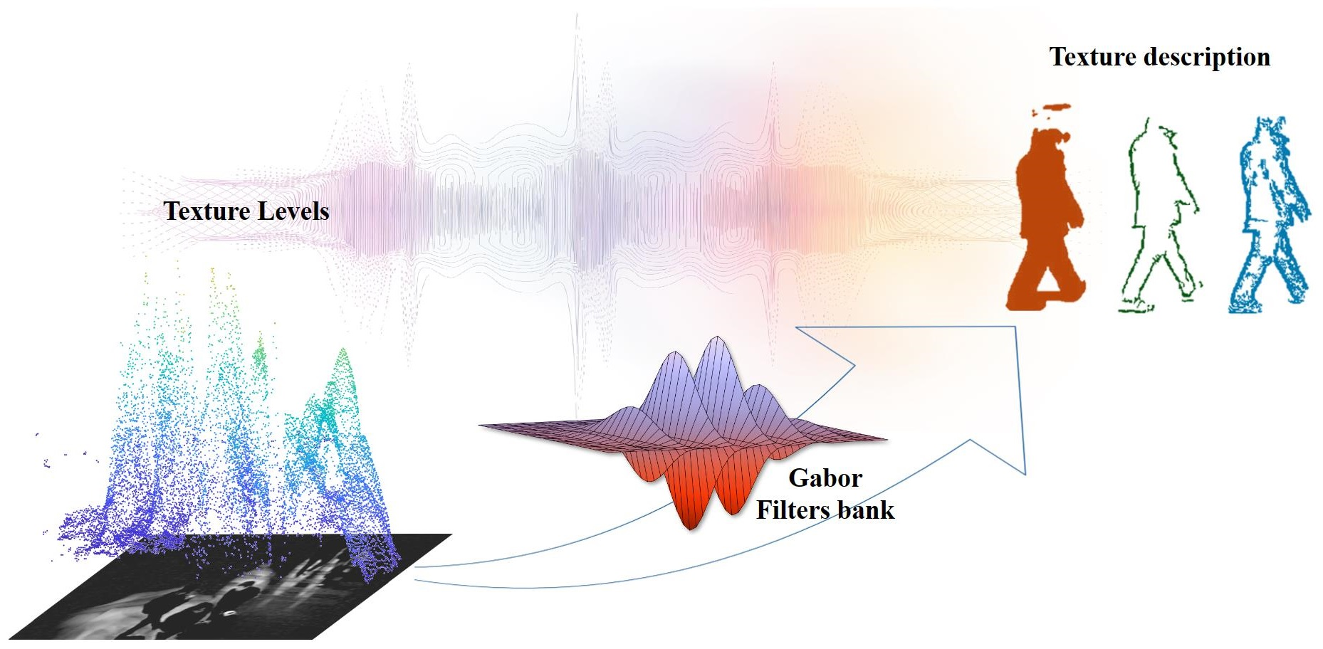
This paper proposes a background subtraction method based on local texture analysis. We assume that the discrete topological surface of the scene satisfies a specific frequency and direction of the Gabor filter bank. The Gabor filter is a linear filter mainly used for texture analysis and discrimination. In its two-dimensional representation, it is a Gaussian kernel function modulated by a sine wave, characterized by the parameters $\lambda ,{\sigma }_x,{\sigma }_y,\theta$ and $\varphi$. In this work, we use it as a texture descriptor. We propose to use the magnitude and phase of the filter to characterize the information that is not sensitive to light changes and build a background model. Based on the results, our method maintains the invariance of subtle changes in light. We assess computational efficiency by processing image series of varying sizes and resolutions. Our test is run on Intel(R) Core i7-7500U CPU with 32.0 GB RAM, achieving a processing rate of 10 frames per second. Upon repeating the experiments, variability in the execution times for each series is observed, which is why it is decided to carry out 30 repetitions, analyzing a total of 181,470 images. The purpose of this is to calculate descriptive statistics, thus obtaining the following results showed in

Table 1. Statistical description of computational efficiency.

Statistics	$640\times 480$	$720\times 576$	$360\times 240$	$320\times 240$
Images evaluated per scene	1200	1700	2050	1099
Average (frames/second)	4.70	3.65	3.95	3.95
Standard deviation (frames/second)	1.26	1.12	1.24	1.44
Minimum (frames/second)	2.73	1.95	2.14	2.37
25% (frames/second)	4.08	3.21	3.36	3.41
50% (frames/second)	4.40	3.37	3.56	3.61
75% (frames/second)	4.70	3.57	3.93	3.79
Maximum (frames/second)	8.40	7.19	7.69	8.31

.

While the proposed method may not achieve the same level of performance as deep learning approaches, it offers several advantages that make it a valuable alternative in certain scenarios. For example, the method is particularly useful when the traditional method cannot handle situations where an object’s color intensity and texture are similar to its surroundings. The proposed method is also invariant to light changes, a common challenge in video surveillance systems. Moreover, the proposed method is computationally efficient and can process video data in real time, making it a faster alternative to deep learning approaches that require large amounts of computational resources and training data. These advantages suggest that the proposed method may be more suitable for real-time object detection and tracking applications, such as video surveillance systems.

The main contributions of this work are (i) the spatio-temporal algorithm that incorporates statistical moments into the Gabor filter bank, (ii) overcoming the shadow detection problem, and (iii) the segmentation of objects with uniform texture around the environment.

The rest of this document is organized as follows. Section 2 describes the theoretical aspects, and Section 3 describes the experimental model, in which texture analysis and motion detection are performed. Section 4 presents the experiments and results. Section 5 discusses the results, and Section 6 presents the conclusion and limitations of the approach.

2. Theoretical Considerations

2.1. Texture Index

An essential part of background modeling is understanding what a texture is and how to quantify it. Although a formal definition has not yet been reported in the literature, authors have classified it as regions composed of points, edges, ellipses, circles, or lines called primitives. It is also defined as the intersection of random and possibly periodic areas [55,56]. It is also defined as the color or intensity distribution [57]. According to [58], variations in intensity, perspective, uniformity, directionality, or scale changes must also be considered. So dealing with texture is a complex issue since it involves the characterization of density, thickness, roughness, or intensity, both in micro and macro textures, irregular or regular and periodical or quasi-periodic [59]. The dataset used in the experiments are explained in Section 3.1.

Another crucial aspect to consider is acquisition noise. When the image is digitized or sampled, noise is generated in the analog-to-digital converter due to an insufficient quantization level. Generally, the camera sensor is 8-bit, which reduces the effective dynamic range of the sensor, thereby producing false contours in the image that are detected as textures.

The question is how to identify the edges that represent the texture. Because randomness leads to subtle changes in intensity levels, detecting these changes can lead to orientation measurements, in which sudden or discontinuous changes can be detected. Generally, the texture depends on the frequency of pixel tones, directionality, and contrast.

In this work, we consider that the texture is the variability of the color pixel intensity. This is determined by the frequency and size of the area affected by the Gaussian function of the Gabor filter.

2.2. Gabor Filter

The Gabor filter bank is one of the functions that allow the density [60], thickness, or directionality of sudden and subtle intensity changes [61] to be characterized and is suitable for texture analysis. The 2-D Gabor function is composed of an envelope function and a carrier. The Gaussian function, commonly called the envelope, is shown in Equation (1):

$$\begin{array}{c}{E}_{\lambda ,\sigma }=\eta ·{exp}^{\left[\left(-\frac{u^2}{2{\sigma }_x^2}-\frac{v^2}{2{\sigma }_y^2}\right)\right]}\hfill \end{array}$$

(1)

where $\eta =\frac{1}{2\pi \lambda ,{\sigma }_x{\sigma }_y}$. ${\sigma }_x$ and ${\sigma }_y$ represent the standard deviation of the Gaussian distribution on the $x$-axis and $y$-axis, and the parameter $\lambda$ represents the filter wavelength. Then, u and v are the Cartesian coordinates of the spatial frequency given by Equation (2):

$$\begin{array}{c}u=x\cos \left(\theta \right)+y\sin \left(\theta \right)\hfill \\ \\ v=y\sin \left(\theta \right)-x\cos \left(\theta \right)\hfill \end{array}$$

(2)

while the carrier function is shown in Equation (3):

$$\begin{array}{c}{C}_{\lambda ,\varphi }=e^{j\omega }\hfill \end{array}$$

(3)

where $\omega =2\pi \frac{u}{\lambda }+\varphi$.

The parameter $\varphi$ represents the phase shift of the complex exponent. The expression $e^{j\omega }$ can be defined as two independent functions, one corresponding to the real part $\left(\cos \omega \right)$ and the other corresponding to the imaginary part $\left(\sin \omega \right)$. So, the Gabor nucleus is defined by Equation (4)

$$\begin{array}{c}{G}_{\lambda ,\theta ,\varphi }=E_{\lambda ,\sigma }·C_{\lambda ,\varphi }\hfill \end{array}$$

(4)

This function is shown in Figure 1. According to the value of $\lambda$, different frequencies can be obtained, and each frequency determines low–pass filter (large $\lambda$), high–pass filter (small $\lambda$) or band–pass filter.

The parameters ${\sigma }_x$ and ${\sigma }_y$ make the Gaussian function increase or decrease in any of its axes, which means that if the Gaussian function extends more on the x-axis than on y-axis, and vice versa, the noise and edges will be attenuated in that axis. However, if the Gaussian term is small, the image’s smoothness will be low, and the sine signal will obtain fewer sampling points.

Finally, the Gabor transformation is shown in Equation (5), which is obtained from the convolution between the image and the Gabor nucleus:

$$\begin{array}{c}{\rm Y}=I_i\left(x\right)\ast G_{\lambda ,\theta ,\varphi }.\hfill \end{array}$$

(5)

Since this function has a real number term (${{\rm Y}}_r$) and a complex number term (${{\rm Y}}_c$), the amplitude $M_i$ and the phase $P_i$ can be obtained as shown in Equations (6) and (7):

$$\begin{array}{c}{M}_i=\sqrt{{{\rm Y}}_r^2+{{\rm Y}}_c^2}\hfill \end{array}$$

(6)

$$\begin{array}{c}{P}_i={tan}^{-1}\left(\frac{{{\rm Y}}_c}{{{\rm Y}}_r}\right)\hfill \end{array}$$

(7)

The terms $M_i$ and $P_i$ are essential because they will define the structure and texture of the object, respectively.

2.3. Statistical Moments

Given the $M_i$ and $P_i$ distributions, the statistical moment r is used to observe the variability of the distribution and calculate the standard deviation. This will allow quantifying the information and distinguishing between the objects in the background and the foreground. According to [62], the r moment is defined in Equation (8):

$$\begin{array}{c}{m}_r={\sum }_{i=1}^N{\left(x_i-\overline{x}\right)}^r·P_b\left(I_i\right)\hfill \end{array}$$

(8)

where N is the total number of elements, $x_i$ is the sample values, $\overline{x}$ is the arithmetic mean of $x_i$, $I_i$ is the color intensity, $P_b\left(I_i\right)$ is the probability, and the r-th moment is represented by r. The first moment ($r=1$) refers to the expected probability. The second moment is the variance and measures the region’s smoothness. The third moment is known as bias and is a measure of displacement; the fourth, or kurtosis provides a measure of uniformity. Higher-order moments can also be used, but they have no representation.

3. Materials and Methods

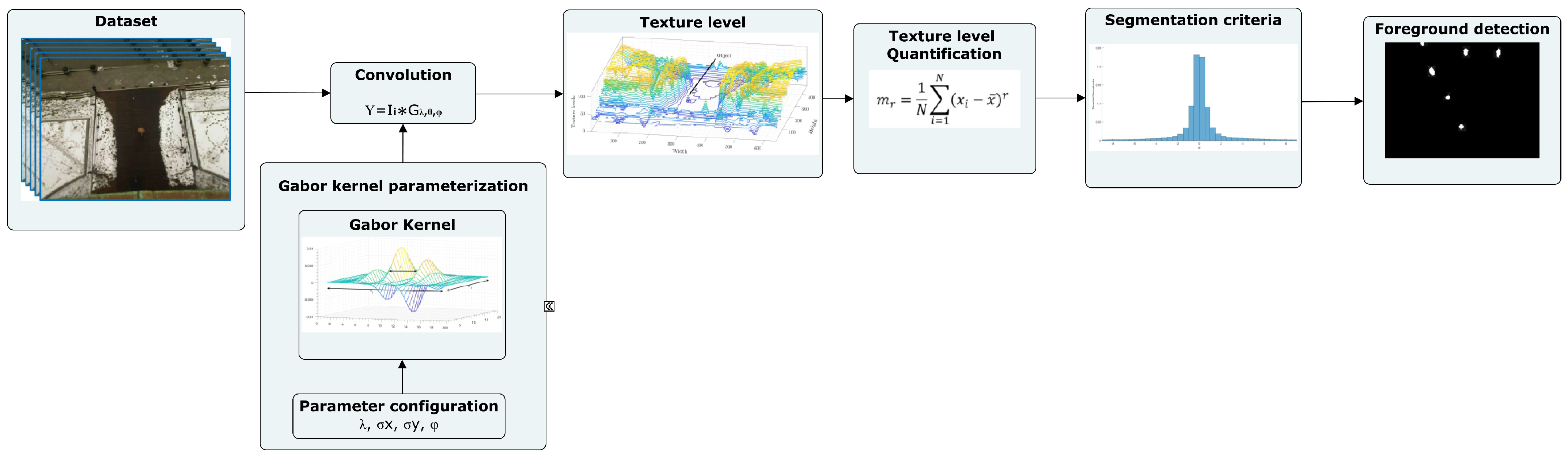
This section describes how to perform background subtraction of our method called GMBSM. Section 3.1 describes the dataset used and the scene’s challenges. Section 3.2 explains the construction of the Gabor kernel for texture characterization. Section 3.3 describes texture-level quantization, and Section 3.4 describes foreground detection. Figure 2 shows the process.

3.1. Dataset

Scene $S_1$. We use the dataset in [63] to analyze a sequence of 500 images with $640\times 480$ pixels dimensions. This scene consists of a fixed camera that can see the ground floor. According to the author, the most notable feature is the constantly changing lighting due to the position of the sun, artificial light sources, and shadows cast by some buildings.

Scene $S_2$. To deepen our analysis, we extract 700 images with a size of $720\times 576$ pixels from the PETS database [64]. This scene includes scattered people walking randomly in bright, dark jackets of uniform and non-uniform textures.

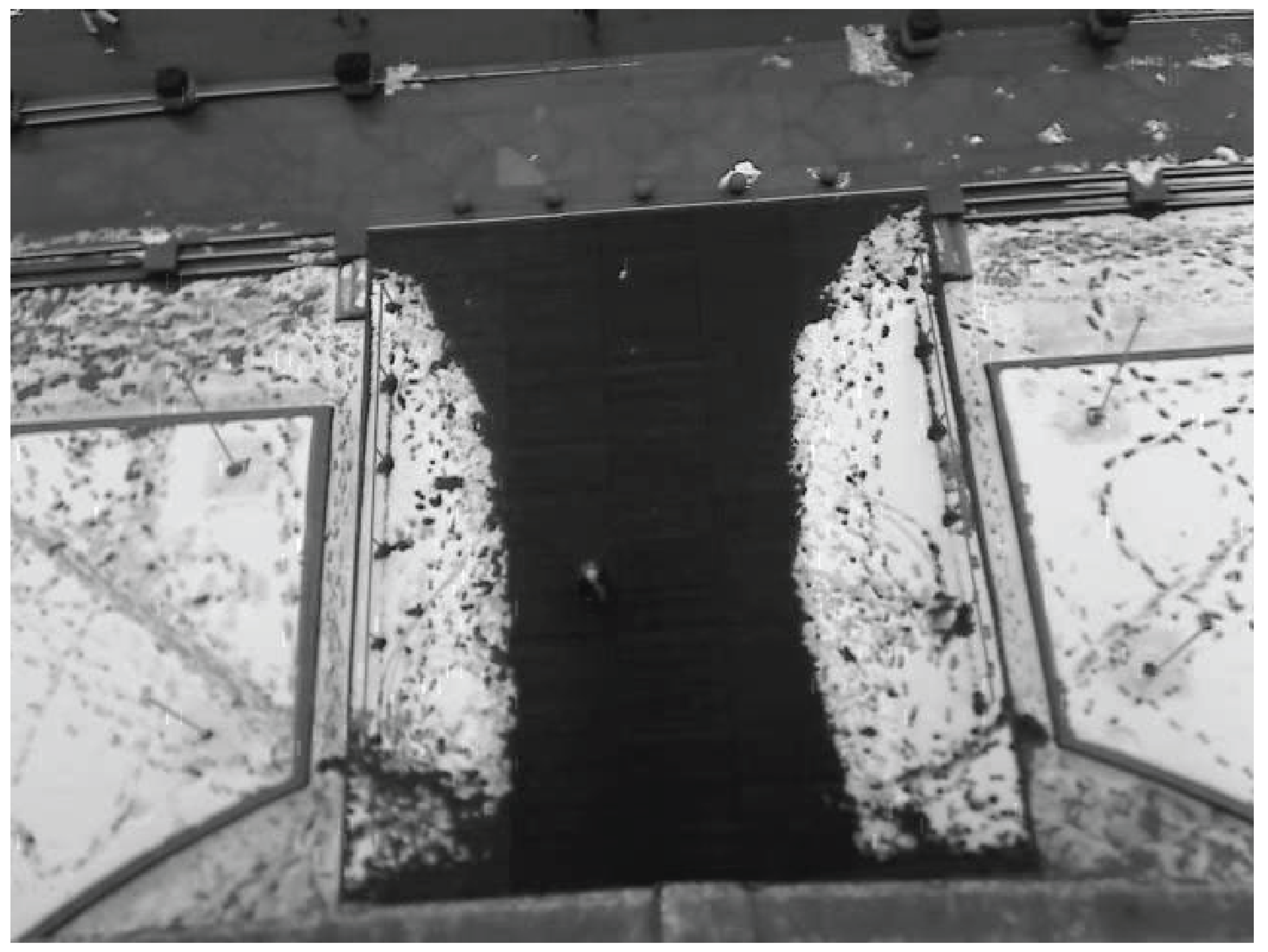
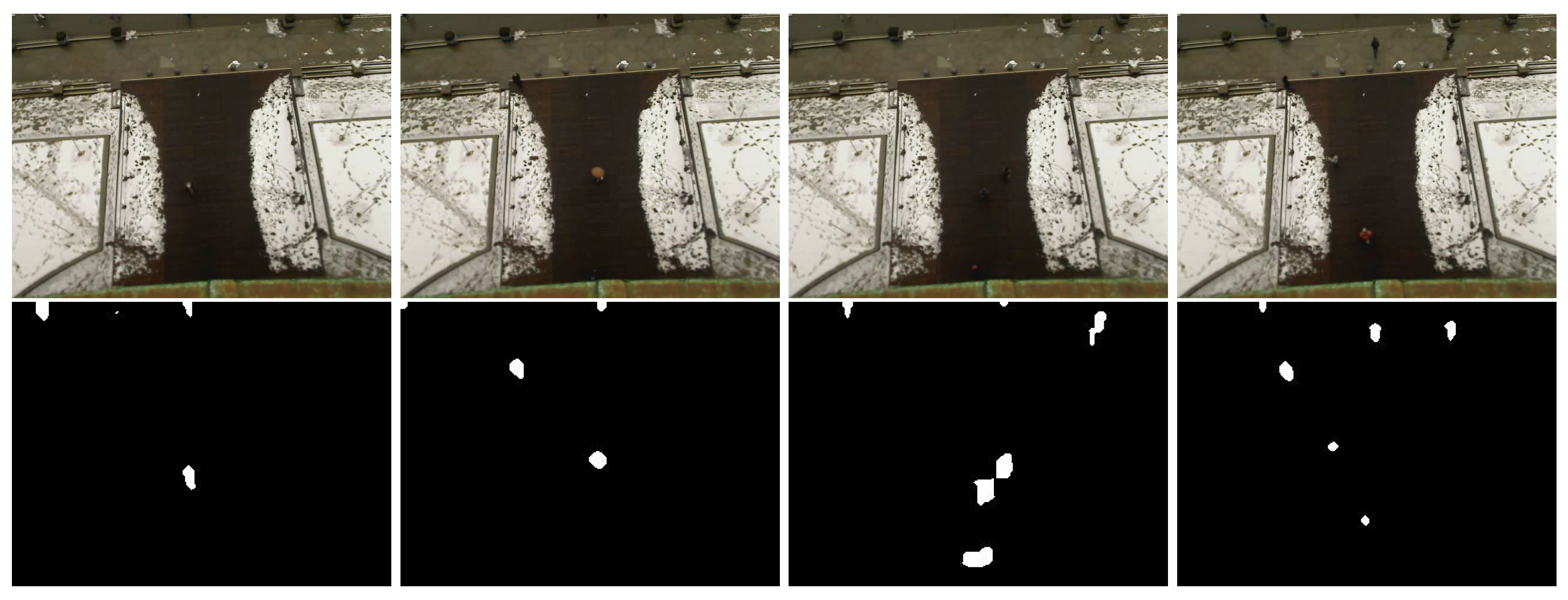
Scene $S_3$. The scene involves people walking through a train station while someone stops and leaves an object on the floor. We choose this scene because shadows and reflections are present due to the lighting conditions. In addition, in some areas of the image, the intensity of the background and the object’s intensity are similar. These effects cause other models to consider that the objects and the background have the same structure. The image size of this sequence is $720\times 576$ pixels.

Scene $S_4$. The traffic flow shows some shadows on the highway from the sun’s position. In addition, dynamic backgrounds are generated due to the movement of the leaves. The dimensions of these images are $320\times 240$ pixels.

Scene $S_5$. A man walked into the office, picked up a book, read it, and left the room in this scene. There are some difficulties here, such as light changes and the color intensity of the clothes relative to the background. The dimensions of these images are $360\times 240$ pixels.

Scene $S_6$. This scene shows some people walking or cycling through the park. The challenge in this scene is the over-illumination and under-sampling of the sequence. The dimensions of these images are $360\times 240$ pixels.

The images of the $S_3$ to $S_6$ scenes are obtained from the dataset in [65].

3.2. Gabor Kernel Parameterization

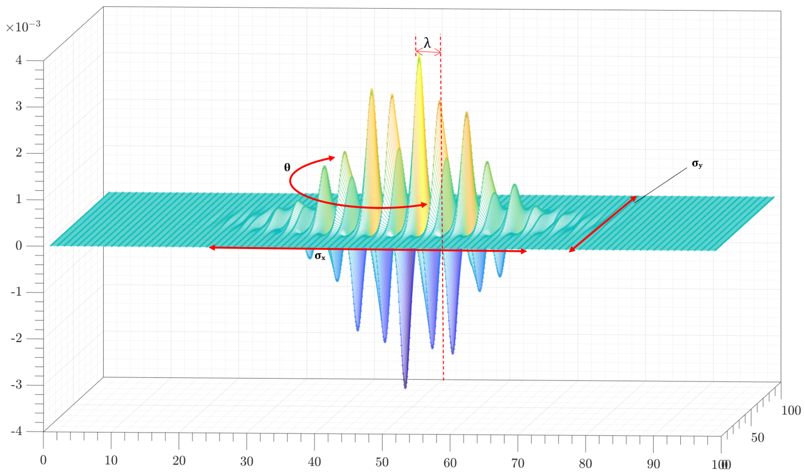
The Gabor function depends on parameters $\lambda$, ${\sigma }_{x,y}$, $\varphi$ and $\theta$, which produce different effects on the image. Both the carrier function and the envelope are in function of $\lambda$, which means that when you have a large $\lambda$ value, the frequency of the envelope is lower. In modeling terms, the filter will attenuate objects with thin edges. However, if the lambda is small, it will have a higher frequency, which allows the filter to attenuate coarse edges so that more details can be visualized but with a higher sensitivity to noise.

On the other hand, ${\sigma }_x$ and ${\sigma }_y$ make the Gaussian term $E_{\lambda ,\sigma }$ large or small in some of its axes, which means that if the Gaussian function extends more on the x-axis than on the y-axis, and vice versa, the noise and edges on that axis will be dimmed on that axis. However, if the Gaussian term is small, the image’s smoothness will be low and noisy.

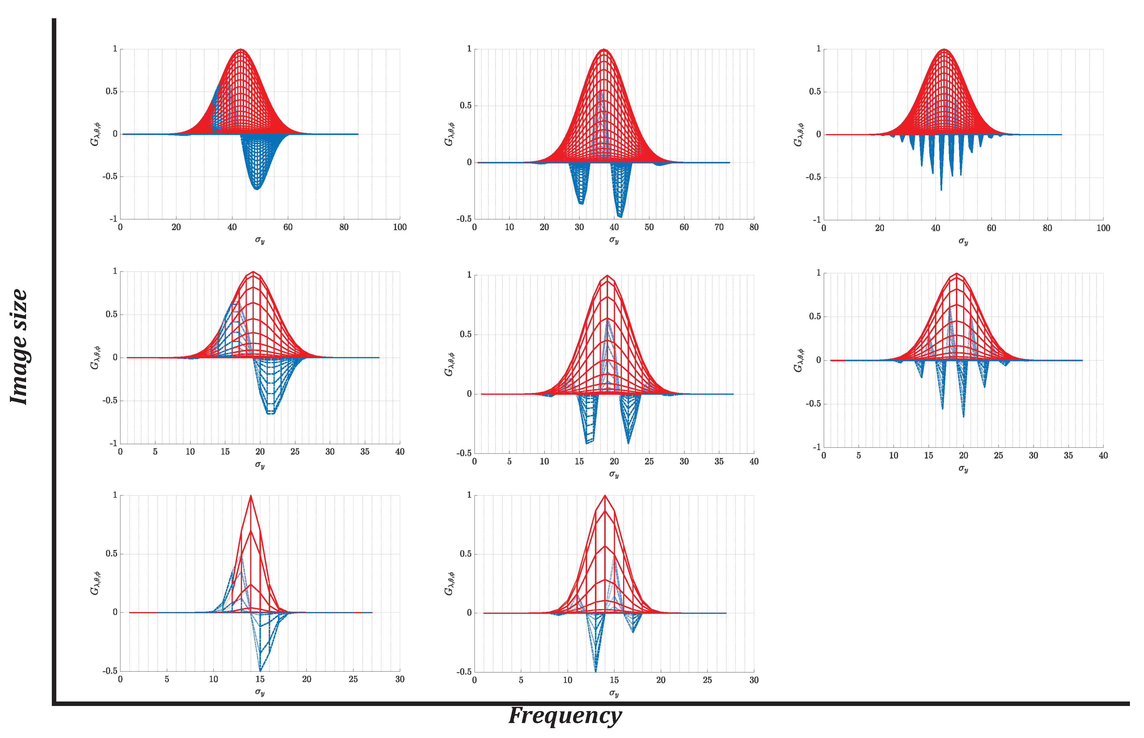
In Figure 3, we show two distributions: $\left(1\right)$ the Gaussian function, whose size depends on ${\sigma }_{x,y}$, and $\left(2\right)$ the relative frequencies of the Gabor filter, where the peak value both positive and negative represent sampling points. Then, as can be seen in the figure, the larger the image size, the higher the density of the Gaussian required. In this way, the noise attenuation is greater. And the smaller the image size, the lower the frequency and density required, but this response will generate more noise and possible false edges.

3.3. Texture Level Maps

Generally, a background model represents a stationary or near-stationary scene with structured elements in an uniform area. Where the light changes of a sequence of images $Q\left(t\right)=\left\{I_1,I_2,I_2,\dots ,I_n\right\}$ are mainly characterized and quantified, each region of $I_i{\left(x\right)}_{m\times n}$ presents a variation of intensity in the pixel values ($x=\left[x_m,y_n\right]$).

So, it is assumed that when a moving object ($O_k$) passes through the scene ($B_k$), it will cause that scene structure to change.

In Figure 4, a scene is observed in which an object of interest $\left(O_k\right)$ can be seen with an intensity value similar to its surrounding environment. This fact is a problem because it is difficult to distinguish between objects and scenes.

Figure 3. Gabor filter size–frequency ratio. This figure shows the comparison between the size of the envelope function (the Gaussian distribution in red) and the response of $G_{\lambda ,\theta ,\varphi }$ (the blue distribution) relative to the size of the image.

Figure 3. Gabor filter size–frequency ratio. This figure shows the comparison between the size of the envelope function (the Gaussian distribution in red) and the response of $G_{\lambda ,\theta ,\varphi }$ (the blue distribution) relative to the size of the image.

Although the intensity levels are similar, we can see that the areas on the scene are not entirely uniform. When another object occludes the scene structure, the structure is altered. Therefore, the distribution and direction of the texture are different. Structural changes are detected using Equations (6) and (7), which allow us to characterize the main frequencies of these regions and represent the structure of the perceived texture. The relative frequency of the Gabor filter’s three–dimensional projection corresponds to the scene’s change. 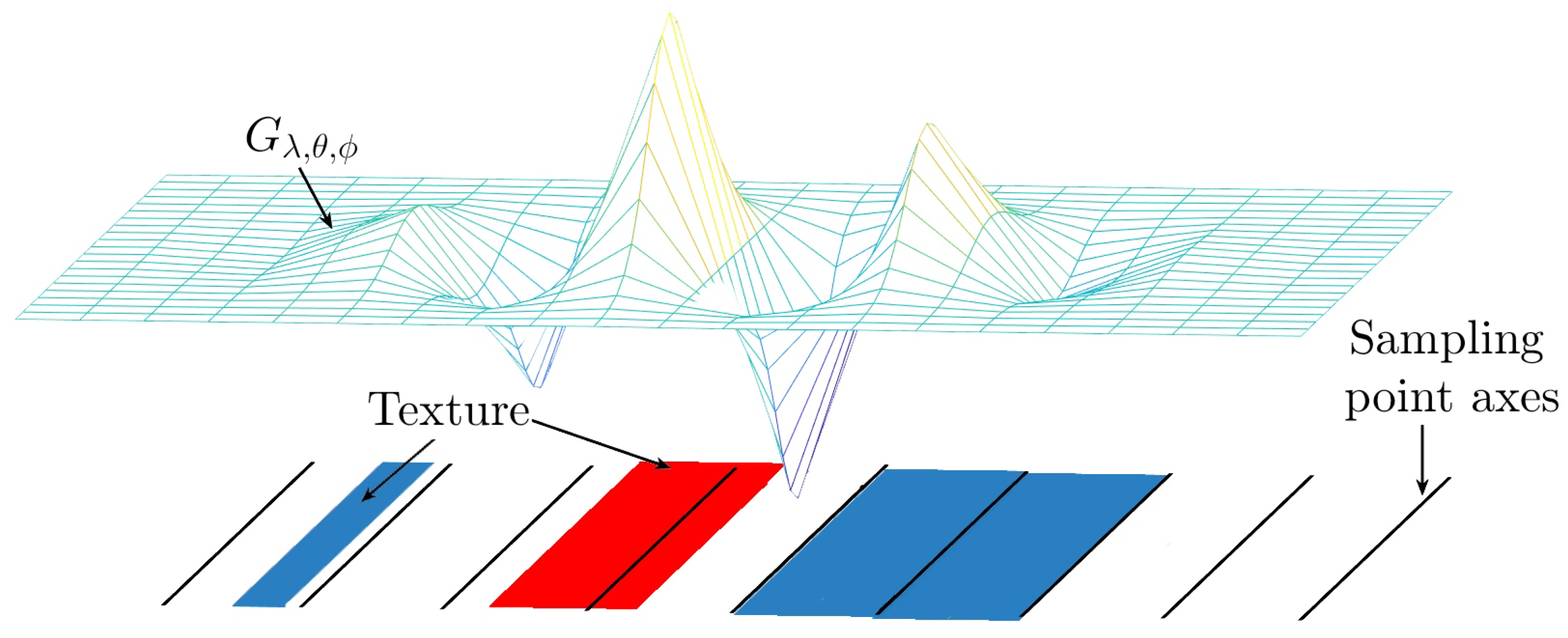Figure 5 shows the texture detected by the filter (red segment) and the not detected texture (blue segments).

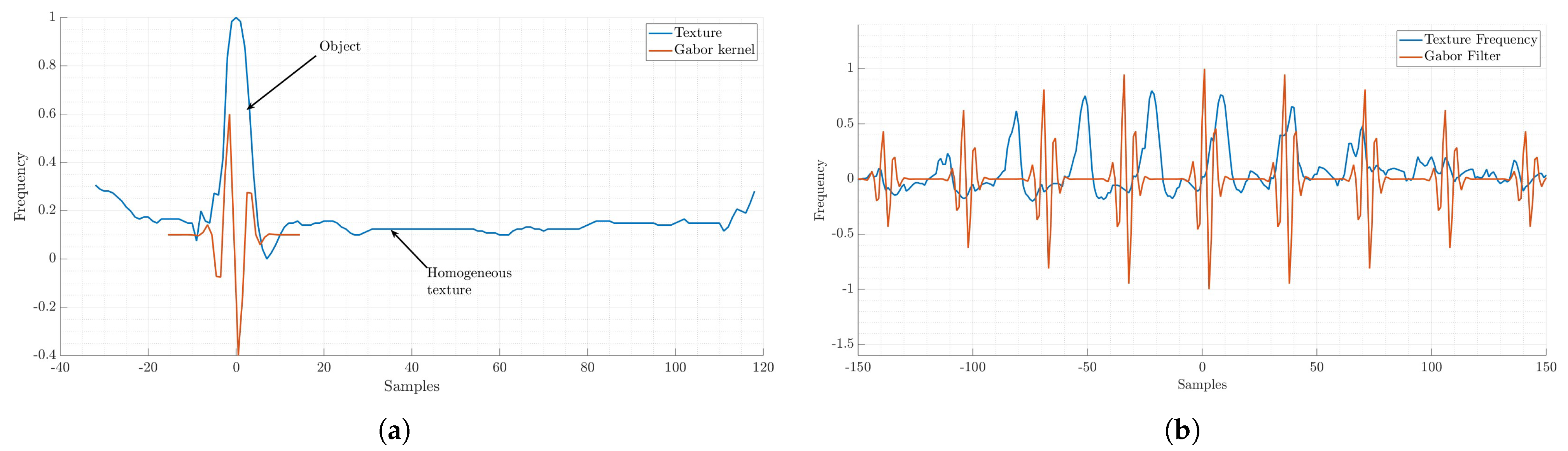
The frequency of the uniform and non–uniform region and the frequency of the Gabor kernel are shown in Figure 6. The maximum values, both positive and negative, represent sampling points. And they measure the texture deformation in the object’s structure; this effect is shown in Figure 6a. Meanwhile, Figure 6b shows when the structure is periodical, and the frequency is similar to the Gabor filter. These structures will not be recognized because the detected changes are not so significant that the filter will attenuate them.

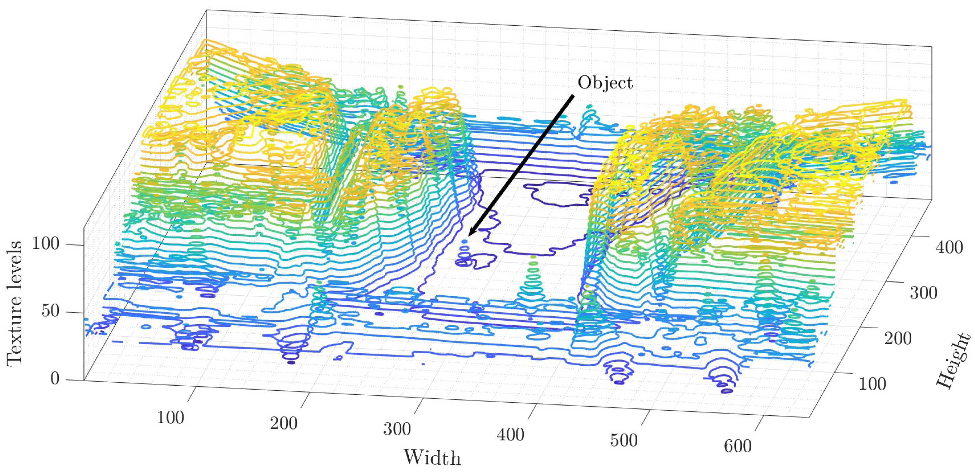
When the Gabor filter is applied, a representation is obtained in the frequency and orientation domain, allowing the identification and characterization of different levels and patterns of texture. The extracted features are essentially a decomposition of the image into components that highlight the texture levels, providing a detailed description of the textures in different scales and orientations. The texture level map obtained is represented in Figure 7, where a subtle change of $O_k$ with respect to $B_k$ is appreciated.

3.4. Texture Level Quantification

To obtain a more uniform area, the r-th moment is calculated. In this way, the texture level is quantified according to the statistical model. In Equation (9), the second statistical moment is used because the average value provides a smooth area:

$$\begin{array}{c}\xi \left(X\right)={\left[F\left(X\right)\right]}^2·P_b\left(X\right)\hfill \end{array}$$

(9)

where $\xi$ represents the quantized texture, $F\left(X\right)\leftarrow X-\overline{X}$, $\overline{X}$ is the average of the n distributions of the $M_i$ and $P_i$ texture map, and X is the latest distribution of the texture map.

The resulting surface is shown in Figure 8, which reflects the distribution of moments in the scene. While the scene distribution appears almost homogeneous, the object distribution shows a greater dispersion in its surroundings, so it is now possible to compare the data variability. According to these distributions, the movement can be detectable.

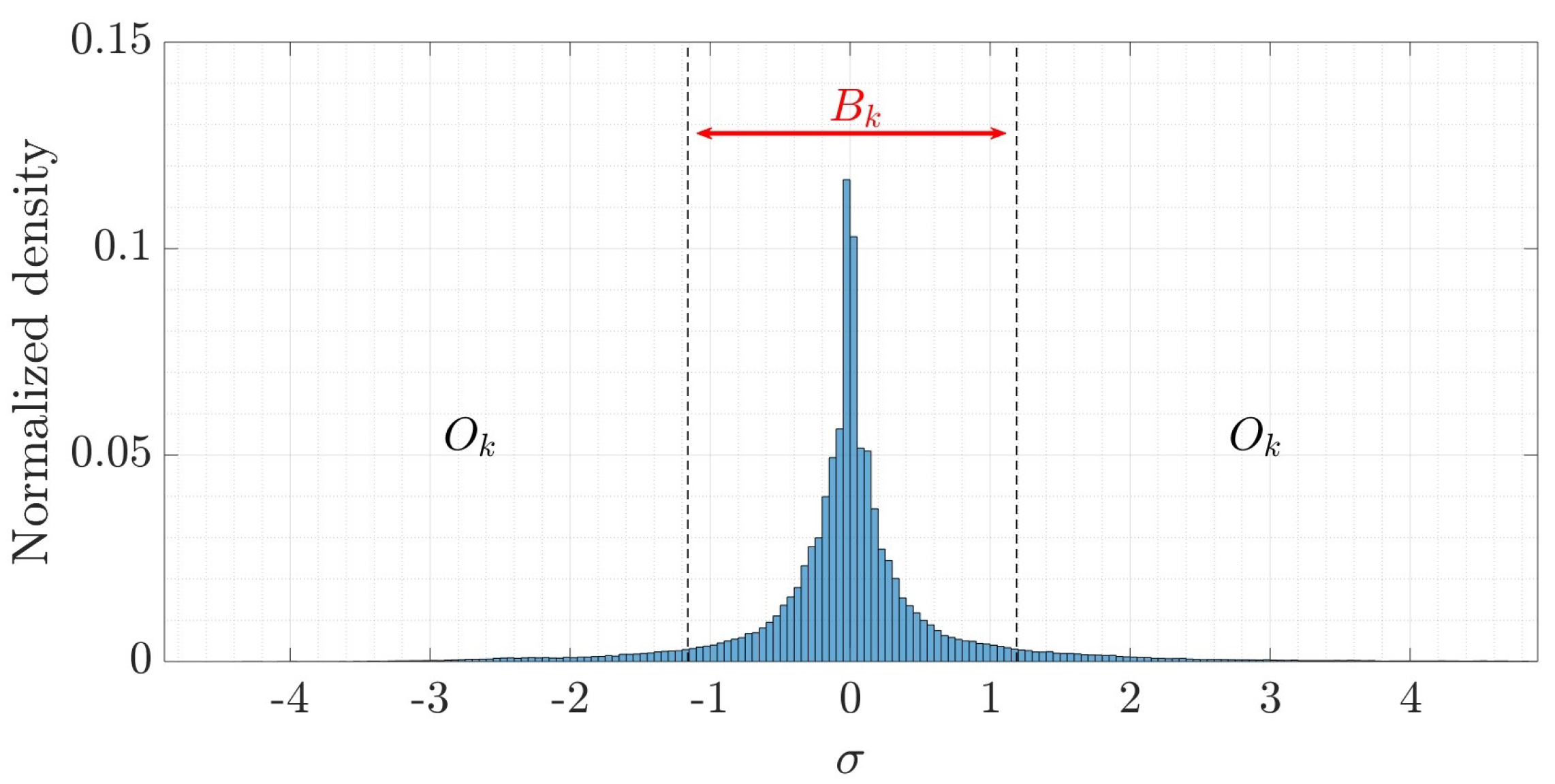
3.5. Segmentation Criteria

Finally, a threshold is chosen to distinguish between stationary $\left(B_k\right)$ and non–stationary objects $\left(O_k\right)$ because the scene now exhibits the distribution shown in Figure 9.

The objects that are in motion can be located from $\pm \sigma$. In this sense, $\sigma$ represents the threshold of stationary objects, which is between $\left[-\sigma ,\sigma \right]$, and moving objects can be determined between $\left(\pm \sigma ,\pm \infty \right)$. Therefore, $k\sigma$ is a function of the confidence interval of the texture distribution we want to compare.

The steps of the background subtraction algorithm are summarized in  Algorithm  1. It should be noted that the analysis is based on the texture of the object, the real term of the filter is used to obtain the object’s structure, and the filter’s imaginary term explains the texture in detail. If there are subtle changes, they can be modeled with any Gabor filter frequency.

Algorithm 1: Texture analysis algorithm

4. Results

This section presents the experimental results of the proposed method. The first experiments consist of adjusting the filter parameters to characterize the light changes in the texture, that is, the number of details in the image that will be used for object analysis, so it is important to adjust the frequency value because an excess of texture may not be as relevant when performing the analysis.

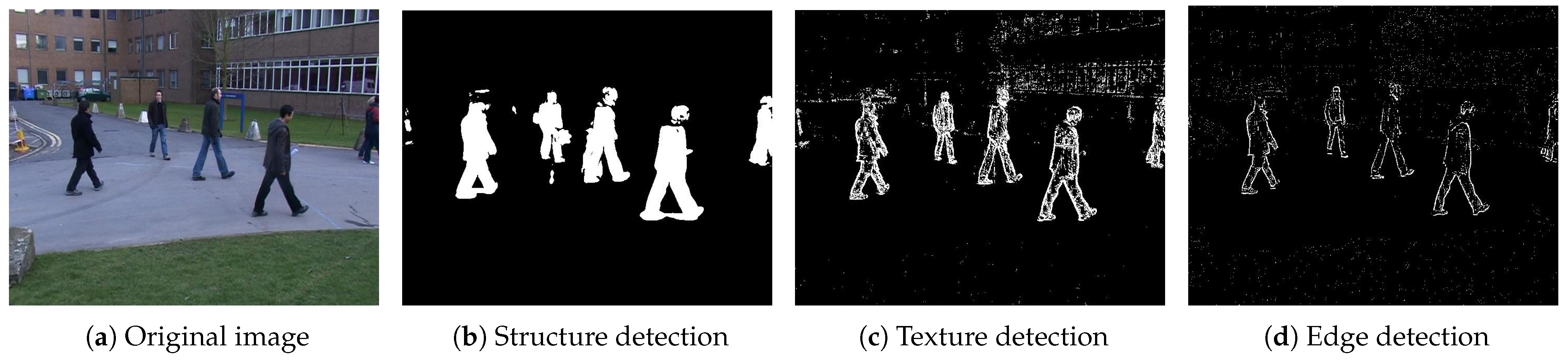
Figure 10 shows the results of the level texture analysis of the scene $S_1$, where both the object and the background distributions are similar. The parameters or this scene are ${\sigma }_x=3$ and ${\sigma }_y=3$, $\varphi =0$ and 24 orientations with an angular displacement of 15.

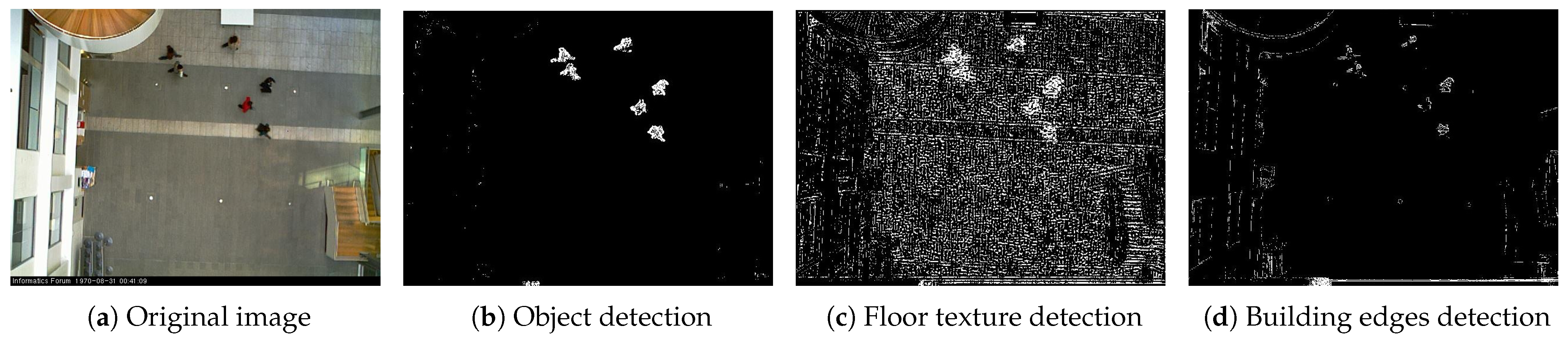
The result below corresponds to scene $S_2$. Different values for $\lambda$ are used to enhance the texture of people (Figure 11b), to enhance the texture of the floor (Figure 11c), and to enhance the edges of buildings (Figure 11d). The influence of these $\lambda$ values can be seen in Figure 11. The parameters that characterize this scene are as follows: Gaussian function value ${\sigma }_x=3.35$ and ${\sigma }_y=1.675$, while $\varphi =0$. In addition, 24 orientations with an angular displacement of 15 degrees are used.

We try to focus on the object’s structure, the texture of the object’s clothes, and the object’s edge. The results are shown in Figure 12.

The parameter values of the Gaussian function used are ${\sigma }_x=6.25$, ${\sigma }_y=1.45$, and $\varphi =0$. Focusing on analyzing different scene levels can reduce the amount of data and only focus on the specific object information. According to the displayed results, adjusting the $\lambda$ value allows the filter to attenuate light changes so that the texture of objects on different levels can be specified to segment them.

We analyze sequences of 900 images for each activity, and the results from our proposal are compared with other methods, such as $\mathsf{\Sigma }\mathsf{\Delta }$ [22], DMD [39], MRFMD [23], DSTEI [26], Eigen-Background [30], SOBS [33], SWCD [40], ViBe [47], GMM [51] and DEU [67]. The results analysis can be seen in

Table 2. Comparison of the results of background subtraction methods.

Method	S3	S4	S5	S6
Image
Groundtruth
DEU
DMD
DSTEI
Eigen-Background Subtraction
GMM
MRFMD
$\mathsf{\Sigma }\mathsf{\Delta }$
SOBS
SWCD
ViBe
GMBSM

.

According to the results, in $S_3$, the proposed method helps to reduce the effects produced by shadows while preserving most of the structure, but a value of $\lambda =1.5$ causes the filter to be susceptible to noise, and objects that are not in motion can be seen. In $S_4$, the vehicle structure is preserved, but the disadvantage is that the light changes of the leaves are detected as a movement. In scenario $S_5$, unlike the other methods, our proposal can obtain a large part of the object structure without noise or deformations. Finally, in $S_6$, there is an acquisition error because the speed of movement of the cyclist is greater than the speed of acquisition of the images, so the cyclist is not clearly seen. Nevertheless, we obtained good results because the complete structure of the cyclist can be appreciated regardless of the shadow and noise; classic noise reduction methods can minimize noise reduction and residual. The morphological closing method can be applied to obtain a complete object structure if necessary.

The parameters used in each model are shown in

Table 3. Background model parameters.

Method	Parameters
DSTEI	$size=3\times 3\times 5$	$Q=100$	$T_h=20$
Eigen Background	$N=28$	$\mathsf{\Sigma }=3$
MRFMD	${\beta }_s=20$	${\beta }_p=10$	${\beta }_f=30$	$\alpha =20$
$\mathsf{\Sigma }\mathsf{\Delta }$	${\mu }_t=3$
SOBS	$n=3$	${ϵ}_2=0.03$	${\gamma }_f=0.07$	${\beta }_f=1$	${\tau }_S=0.1$	${\tau }_H=10$
SWCD	$N=35$	$T_l=2$	$T_u=0.07$	$R=0.01$
ViBe	$N=205$	$\sigma =20$	$\rho =16$
DMD	$D_t=1$	$T_h=0.25$
DEU	$\rho =0.9$	$\alpha =0.1$
GMM	$\sigma =3.5$	$\rho =0.9967$
GMBSM	$\sigma =1.5$	$\varphi =0$	$\lambda =0.35$	${\sigma }_x=3.25$	${\sigma }_y=1.5$

, which were reported by each author so that each model maintains the best performance of its algorithm.

In addition to the qualitative tests performed, we conducted quantitative tests on 3600 images, corresponding to a sequence of 900 images from each scene, to estimate the rates of true positives and false positives. Although there are different ways to evaluate performance, the evaluation here is performed at the pixel level. In addition to measurement accuracy and sensitivity, the indicators described below are also used to evaluate and verify data. According to [68], these are defined as follows.

Sensitivity (also known as True Positive Rate or Recall): This metric measures the proportion of actual positives that are correctly identified as such. It is calculated as:

$$Sensitivity=\frac{T_P}{T_P+F_N}$$

(10)

Specificity: It measures the proportion of actual negatives that are correctly identified. It is calculated as:

$$Specifity=\frac{T_N}{T_N+F_P}$$

(11)

False Positive Rate (FPR): This is the proportion of actual negatives that are incorrectly identified as positives. It is calculated as:

$$FPR=\frac{F_P}{T_N+F_P}$$

(12)

False Negative Rate (FNR): This metric measures the proportion of actual positives that are incorrectly identified as negatives. It is calculated as:

$$FNR=\frac{F_N}{T_P+F_N}$$

(13)

PWC (Percentage of Wrong Classifications): It represents the percentage of all classifications that were incorrect. It is calculated as:

$$PWC=\frac{100\times (F_N+F_P)}{T_P+F_N+F_P+T_N}$$

(14)

Precision (also known as Positive Predictive Value): This metric measures the proportion of identified positives that are actually correct. It is calculated as:

$$Precision=\frac{T_P}{T_P+F_P}$$

(15)

F Measure (or F1 Score): This is the harmonic mean of Precision and Sensitivity. It provides a single score that balances the trade-off between Precision and Recall. It is calculated as:

$$FMeasure=2·\frac{Precision·Sensitivity}{Precision+Sensitivity}$$

(16)

True positive $\left(T_P\right)$ refers to pixels correctly identified as part of the moving object. True negative $\left(T_N\right)$ denotes pixels correctly identified as part of the static background. False positive $\left(F_P\right)$ pertains to pixels incorrectly labeled as part of the moving object when they belong to the background, while false negative $\left(F_N\right)$ refers to pixels incorrectly labeled as background when they are truly part of the moving object.

Table 4. Results obtained when evaluating the methods in $S_3$.

Method	Sensibility	Specificity	FPR	FNR	PWC	Precision	F1 Measure
DEU	0.274	0.984	0.016	0.726	0.301	0.144	0.188
DMD	0.875	0.990	0.010	0.125	1.108	0.472	0.613
DSTEI	0.658	0.984	0.016	0.342	1.751	0.122	0.206
EigenBS	0.437	0.991	0.009	0.563	2.151	0.546	0.486
GMM	0.929	0.991	0.009	0.071	0.989	0.507	0.656
MRFMD	0.735	0.983	0.017	0.265	1.775	0.071	0.130
SDBE	0.830	0.992	0.008	0.170	1.024	0.565	0.673
SOBS	0.929	0.991	0.009	0.071	0.994	0.504	0.654
SWCD	0.890	0.997	0.003	0.110	0.451	0.865	0.877
ViBe	0.883	0.992	0.008	0.117	0.949	0.565	0.689
GMBSM	0.738	0.994	0.006	0.262	1.059	0.668	0.701

and

Table 5. Results obtained when evaluating the methods in $S_4$.

Method	Sensibility	Specificity	FPR	FNR	PWC	Precision	F1 Measure
DEU	0.285	0.981	0.019	0.715	2.667	0.140	0.187
DMD	0.859	0.991	0.009	0.141	1.127	0.585	0.696
DSTEI	0.620	0.980	0.020	0.380	2.103	0.119	0.199
EigenBS	0.364	0.991	0.009	0.636	3.190	0.596	0.452
GMM	0.793	0.993	0.007	0.207	1.086	0.686	0.736
MRFMD	0.912	0.991	0.009	0.088	1.027	0.591	0.717
SDBE	0.688	0.979	0.021	0.312	2.130	0.062	0.113
SOBS	0.817	0.992	0.008	0.183	1.129	0.628	0.710
SWCD	0.914	0.991	0.009	0.086	0.999	0.604	0.727
ViBe	0.878	0.998	0.002	0.122	0.508	0.893	0.886
GMBSM	0.856	0.99	0.008	0.144	0.993	0.660	0.746

compare existing methods and GABSM.

Table 4 shows the results achieved by our method, which achieves a sensitivity of $0.738$. This reflects its efficiency in correctly identifying relevant foreground elements. On the other hand, a specificity of $0.994$ shows the ability to exclude noise generated by reflections. With a misclassification rate of $1.059$, it demonstrates a low error rate in classifying textures, even when they are complex or appear homogeneous with the environment, under variable lighting conditions. These fluctuations in lighting can significantly alter how textures are perceived, representing a challenge for their classification and analysis. Nevertheless, an $F1$ score of $0.701$ evidences that our method is capable not only of recognizing complex texture patterns but also of adapting to the variability caused by changes in lighting.

In Table 5, a sensitivity of $0.856$ is obtained, reflecting our method’s ability to correctly detect objects of interest. Its specificity of $0.99$ and an FPR of $0.008$ demonstrate its efficacy in discarding irrelevant elements, even in a dynamic environment due to the movement of leaves. According to the $F1$ score of $0.746$, our method proves to be effective in facing the complexity of environments influenced by shadows and dynamic movements, such as those generated by moving tree leaves. Additionally, this environment introduces changes in perspective, where the distinction between distant and nearby objects complicates the detection of moving objects due to a fixed Gabor core.

In

Table 6. Results obtained when evaluating the methods in $S_5$.

Method	Sensibility	Specificity	FPR	FNR	PWC	Precision	F1 Measure
DEU	0.380	0.956	0.043	0.619	10.821	0.525	0.440
DMD	0.393	0.922	0.078	0.607	8.648	0.080	0.133
DSTEI	0.598	0.935	0.065	0.402	7.637	0.238	0.341
EigenBS	0.900	0.922	0.078	0.100	7.844	0.060	0.113
GMM	0.940	0.969	0.031	0.060	3.308	0.642	0.763
MRFMD	0.986	0.943	0.057	0.014	5.585	0.331	0.495
SDBE	0.919	0.920	0.080	0.081	8.000	0.038	0.073
SOBS	0.710	0.931	0.069	0.290	7.391	0.183	0.291
SWCD	0.999	0.974	0.026	0.001	2.478	0.701	0.824
ViBe	0.927	0.993	0.007	0.073	1.268	0.920	0.923
GMBSM	0.827	0.988	0.012	0.172	0.578	0.863	0.901

, a sensitivity of $0.827$ and a high specificity of $0.988$ are observed, along with a relatively low FNR of $0.172$ and an FPR of $0.012$. These parameters demonstrate that the GABSM method can adapt to scenarios where moving objects may stop unexpectedly, presenting a problem for traditional background modeling methods. With an accuracy of $0.863$ and an F1 score of $0.901$, GABSM proves its reliability in adapting to such scenarios.

Table 7. Results obtained when evaluating the methods in $S_6$.

Method	Sensibility	Specificity	FPR	FNR	PWC	Precision	F1 Measure
DEU	0.318	0.949	0.051	0.682	6.173	0.096	0.148
DMD	0.742	0.958	0.042	0.258	4.618	0.260	0.385
DSTEI	0.645	0.949	0.051	0.355	5.340	0.088	0.155
EigenBS	0.619	0.978	0.022	0.381	4.211	0.630	0.625
GMM	0.985	0.956	0.044	0.015	4.317	0.227	0.369
MRFMD	0.732	0.947	0.053	0.268	5.413	0.042	0.079
SDBE	0.576	0.956	0.044	0.424	5.227	0.227	0.326
SOBS	0.997	0.979	0.021	0.003	2.016	0.640	0.779
SWCD	0.927	0.993	0.007	0.073	1.054	0.879	0.903
ViBe	0.977	0.978	0.022	0.023	2.245	0.611	0.752
GMBSM	0.829	0.991	0.008	0.171	0.271	0.736	0.780

presents the results obtained in a scenario characterized by acquisition errors and the presence of shadows on moving objects. With a sensitivity of $0.829$, our method can detect foreground moving objects, even in conditions where sampling is not adequate. A specificity of $0.991$ shows its efficiency in differentiating between objects of interest and the background, thus minimizing misdetections caused both by shadows and acquisition errors.

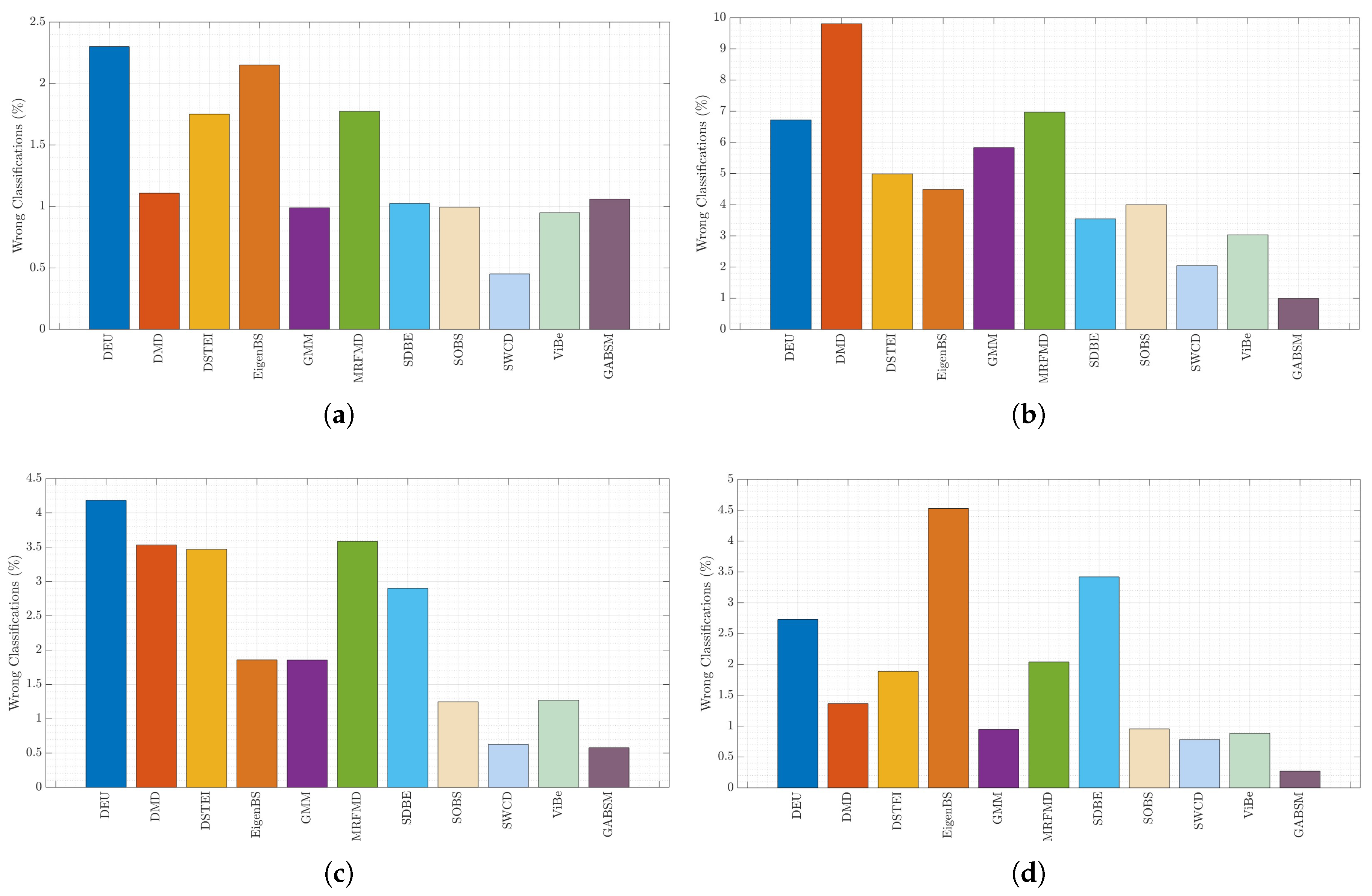
Figure 13 shows the percentage of wrong classifications $\left(PWC\right)$, which shows the deviation error in the scene. This error is caused by the number of false positives $\left(FPR\right)$ and false negatives $\left(FNR\right)$ described.

Figure 13a shows that the proposed method has an error percentage similar to most methods (about $1\%$) due to the change in the object’s perspective. This problem is the main weakness of the Gabor filter because it requires functions $G_{\lambda ,\theta ,\varphi }$ of different sizes and frequencies. This increases the complexity of parameter selection and the processing time. This same problem is shown in Figure 13b. However, in Figure 13c,d, we can see that the percentage of error is lower; this is because the objects in $S_5$ and $S_6$ scenes do not have perspective with respect to the camera. For this reason, the size of the $G_{\lambda ,\theta ,\varphi }$ function is fixed so that the texture can be better modeled. The problem in these scenarios is that they have lower resolution, which means that ${\sigma }_x$ and ${\sigma }_y$ have to be reduced, as well as, therefore, the lambda value. This effect increases the amount of noise detected and therefore impacts the amount of true positives detected.

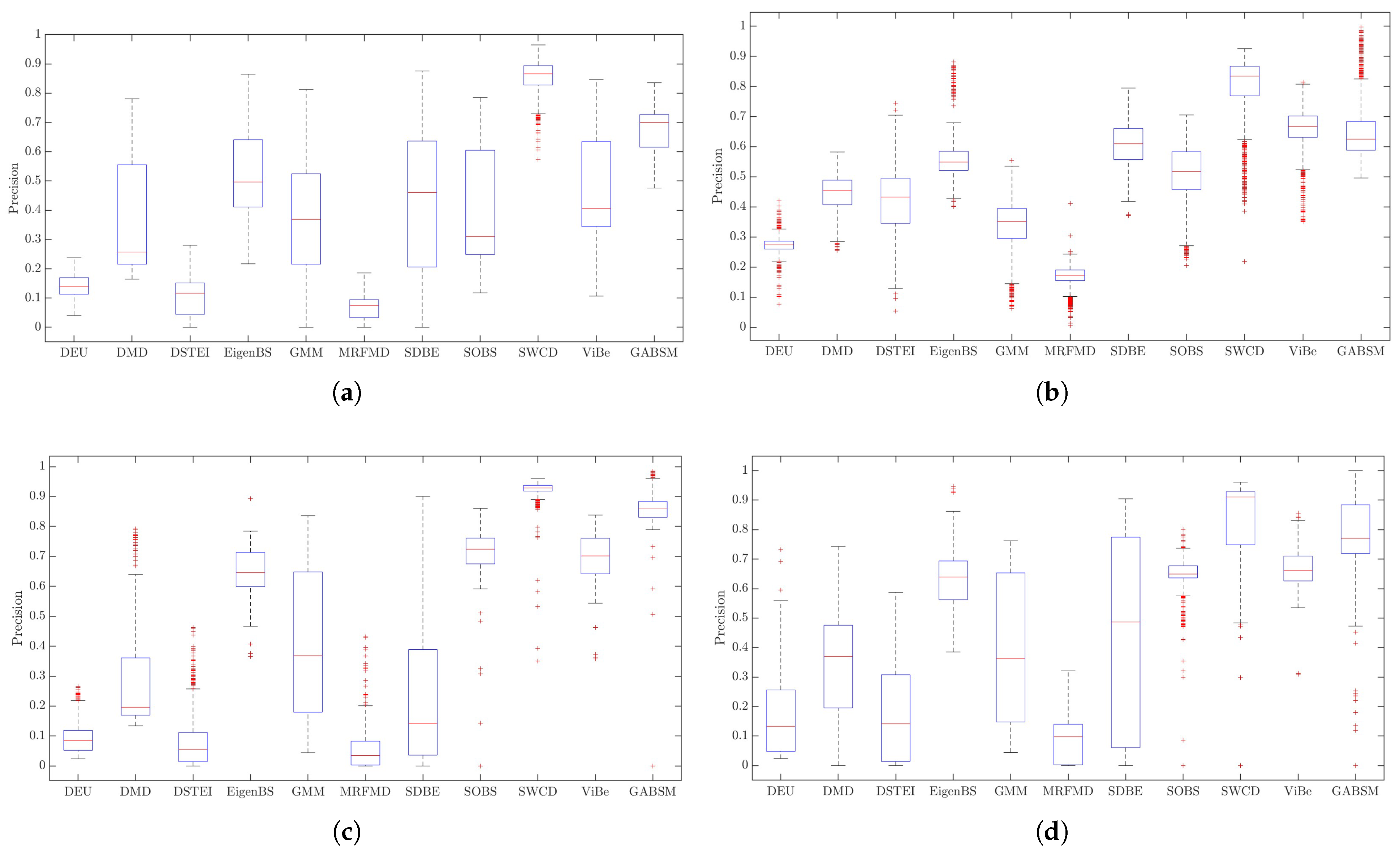
Figure 14 shows the precision of the methods, which helps us to visualize which method provides us with more information about moving objects and minimizes irrelevant information caused by noise, the presence of shadows, or changes in lighting. Although our method has good precision regarding positive predictions, its performance is reduced when the images are smaller or difficult to characterize lighting changes.

5. Discussion

According to the results obtained in Table 2, only methods such as DEU, DSTEI, and RFMD obtained the objects’ contour. The methods DMD, GMM, Sigma-Delta, and SWCD, although they partially preserve the structure of the objects, present loss of information in distant objects and are susceptible to shadows and reflections caused by lighting.From our point of view, the Eigen-Background, SOBS, ViBe, and our GMBSM method provide better results in preserving the object structure, but they cause the loss of information about distant objects. Among them, GMBSM is the best, and the results in Figure 13 and Figure 14 show a lower error percentage and higher accuracy. Nevertheless, distant objects in scenes $S_3$ and $S_4$ will lose information due to the perspective of these scenes.

As mentioned in Section 3.2, a larger object in the image requires a higher density Gaussian so that the noise attenuation is greater. Although the object is smaller, it requires a lower frequency response and Gaussian density, producing more noise and possible false contours. This effect is one of the weaknesses of our method because it requires different G functions to be applied to the scene. This will increase the execution time and the complexity of adjusting the parameters.

The advantages of our method are that (i) the representation of an object whose texture is almost the same as its environment, (ii) it can recover quickly when the object in motion remains stationary, (iii) according to experiments, it exhibits invariance to light changes, and (iv) it allows the analysis of texture levels to obtain different texture details.

However, it also has disadvantages: (i) the proper selection of the size of $\left(G_{\lambda ,\theta ,\varphi }\right)$ depends on the size of the objects in the scene, (ii) experience is required to select the appropriate filter parameters and finally, and (iii) the suggested threshold is not the best method because it depends on the variance of the data, and in the absence of objects, it will only produce noise. These issues are being considered for future work, as well as improvements to the method.

6. Conclusions

We introduced a background subtraction technique that leverages texture-level analysis through the integration of a Gabor filter bank and statistical moments. This approach is differentiated by its capacity to distinguish between foreground and background entities in dynamic scenes, a critical challenge where traditional methods often need to improve. Our method has demonstrated superior performance in maintaining the structural integrity of the objects while effectively addressing gradual changes in lighting, shadows, and scenarios with nearly uniform environmental textures. Our experimental validation exhibited benefits over conventional methods by ensuring lower false detection rates and maintaining high accuracy in object detection across a variety of challenging conditions.

Despite its performance, our method encounters limitations when processing images of reduced size or in scenarios with complex lighting variations. The difficulty in characterizing such changes impacts the algorithm’s performance, suggesting a need for improved strategies in handling small objects or subtle texture variations. Additionally, the reliance on specific Gabor filter parameters and the selection of an optimal threshold for background subtraction present complexities in parameter optimization, potentially restricting the method’s adaptability and ease of implementation across diverse surveillance contexts.

Looking forward, we aim to address these limitations by exploring adaptive parameterization techniques that can dynamically adjust the Gabor filter settings based on the scene’s characteristics. This could enhance the method’s robustness against varied image sizes and complex lighting conditions. Further, we plan to investigate deep learning frameworks that could learn these parameters autonomously, offering a more sophisticated understanding of the scene dynamics. Additionally, integrating multimodal data sources, such as depth information, could enrich the algorithm’s contextual awareness, opening opportunities for more subtle object detection and background modeling. Through these advancements, we aspire to broaden the applicability of our method, making it a more versatile tool for real-time surveillance and motion tracking in an array of real-world settings.

References

1. Liu, H.; Hou, X. Moving Detection Research of Background Frame Difference Based on Gaussian Model. In Proceedings of the 2012 International Conference on Computer Science and Service System, Nanjing, China, 11–13 August 2012; pp. 258–261. [Google Scholar] [CrossRef]
2. Guo, J.; Wang, J.; Bai, R.; Zhang, Y.; Li, Y. A New Moving Object Detection Method Based on Frame-difference and Background Subtraction. IOP Conf. Ser. Mater. Sci. Eng. 2017, 242, 012115. [Google Scholar] [CrossRef]
3. Srivastav, N.; Agrwal, S.L.; Gupta, S.K.; Srivastava, S.R.; Chacko, B.; Sharma, H. Hybrid object detection using improved three frame differencing and background subtraction. In Proceedings of the 7th International Conference on Cloud Computing, Data Science Engineering-Confluence, Uttar Pradesh, India, 12–13 January 2017; pp. 613–617. [Google Scholar] [CrossRef]
4. Roy, S.M.; Ghosh, A. Real-Time Adaptive Histogram Min-Max Bucket (HMMB) Model for Background Subtraction. IEEE Trans. Circuits Syst. Video Technol. 2018, 28, 1513–1525. [Google Scholar] [CrossRef]
5. Sajid, H.; Cheung, S.S. Universal Multimode Background Subtraction. IEEE Trans. Image Process. 2017, 26, 3249–3260. [Google Scholar] [CrossRef]
6. Stauffer, C.; Grimson, W.E.L. Adaptive background mixture models for real-time tracking. In Proceedings of the 1999 IEEE Computer Society Conference on Computer Vision and Pattern Recognition (Cat. No PR00149), Fort Collins, CO, USA, 23–25 June 1999; Volume 2, pp. 246–252. [Google Scholar] [CrossRef]
7. Joy, F.; Vijayakumar, V. An improved Gaussian Mixture Model with post-processing for multiple object detection in surveillance video analytics. Int. J. Electr. Comput. Eng. Syst. 2022, 13, 653–660. [Google Scholar] [CrossRef]
8. Yasir, M.A.; Ali, Y.H. Comparative analysis of GMM, KNN, and ViBe background subtraction algorithms applied in dynamic background scenes of video surveillance system. Eng. Technol. J. 2022, 40, 617–626. [Google Scholar] [CrossRef]
9. Reyana, A.; Kautish, S.; Vibith, A.; Goyal, S. EGMM video surveillance for monitoring urban traffic scenario. Int. J. Intell. Unmanned Syst. 2023, 11, 35–47. [Google Scholar] [CrossRef]
10. Cong, V.D. Extraction and classification of moving objects in robot applications using GMM-based background subtraction and SVMs. J. Braz. Soc. Mech. Sci. Eng. 2023, 45, 317. [Google Scholar] [CrossRef]
11. Rakesh, S.; Hegde, N.P.; Gopalachari, M.V.; Jayaram, D.; Madhu, B.; Hameed, M.A.; Vankdothu, R.; Kumar, L.S. Moving object detection using modified GMM based background subtraction. Meas. Sens. 2023, 30, 100898. [Google Scholar] [CrossRef]
12. Setyoko, B.H.; Noersasongko, E.; Shidik, G.F.; Budiman, F.; Soeleman, M.A.; Andono, P.N. Gaussian Mixture Model in Dynamic Background of Video Sequences for Human Detection. In Proceedings of the 2022 5th International Seminar on Research of Information Technology and Intelligent Systems (ISRITI), Yogyakarta, Indonesia, 8 December 2022; pp. 595–600. [Google Scholar]
13. Aslam, N.; Kolekar, M.H. A Probabilistic Approach for Detecting Human Motion in Video Sequence using Gaussian Mixture Model. In Proceedings of the 2022 2nd International Conference on Emerging Frontiers in Electrical and Electronic Technologies (ICEFEET), Patna, India, 24–25 June 2022; pp. 1–6. [Google Scholar]
14. Bhavani, K.D.; Ukrit, M.F. Human Fall Detection using Gaussian Mixture Model and Fall Motion Mixture Model. In Proceedings of the 2023 5th International Conference on Inventive Research in Computing Applications (ICIRCA), Tamil Nadu, India, 3–5 August 2023; pp. 1814–1818. [Google Scholar]
15. Chetouane, A.; Mabrouk, S.; Jemili, I.; Mosbah, M. Vision-based vehicle detection for road traffic congestion classification. Concurr. Comput. Pract. Exp. 2022, 34, e5983. [Google Scholar] [CrossRef]
16. Indu, T.; Shivani, Y.; Reddy, A.; Pradeep, S. Real-time Classification and Counting of Vehicles from CCTV Videos for Traffic Surveillance Applications. Turk. J. Comput. Math. Educ. 2023, 14, 684–695. [Google Scholar]
17. Boyat, A.; Joshi, B.K. A Review Paper: Noise Models in Digital Image Processing. Signal Image Process. Int. J. 2015, 6, 63–75. [Google Scholar] [CrossRef]
18. Mahmoudpour, S.; Kim, M. Robust foreground detection in sudden illumination change. Electron. Lett. 2016, 52, 441–443. [Google Scholar] [CrossRef]
19. Amitha, V.; Behera, R.K.; Vinuchackravarthy, S.; Krishnan, K. Background Modelling from a Moving Camera. Procedia Comput. Sci. 2015, 58, 289–296. [Google Scholar]
20. Davy, A.; Desolneux, A.; Morel, J. Detection of Small Anomalies on Moving Background. In Proceedings of the 2019 IEEE International Conference on Image Processing (ICIP), Taipei, Taiwan, 22–25 September 2019; pp. 2015–2019. [Google Scholar] [CrossRef]
21. Xu, Y.; Dong, J.; Zhang, B.; Xu, D. Background modeling methods in video analysis: A review and comparative evaluation. CAAI Trans. Intell. Technol. 2016, 1, 43–60. [Google Scholar] [CrossRef]
22. Milla, J.M.; Toral, S.L.; Vargas, M.; Barrero, F.J. Dual-rate background subtraction approach for estimating traffic queue parameters in urban scenes. IET Intell. Transp. Syst. 2013, 7, 122–130. [Google Scholar] [CrossRef]
23. Subudhi, B.N.; Ghosh, S.; Nanda, P.K.; Ghosh, A. Moving object detection using spatio-temporal multilayer compound Markov Random Field and histogram thresholding based change detection. Multimed. Tools Appl. 2017, 76, 1573–7721. [Google Scholar] [CrossRef]
24. Bouwmans, T.; Silva, C.; Marghes, C.; Zitouni, M.S.; Bhaskar, H.; Frelicot, C. On the role and the importance of features for background modeling and foreground detection. Comput. Sci. Rev. 2018, 28, 26–91. [Google Scholar] [CrossRef]
25. Jing, G.; Siong, C.E.; Rajan, D. Foreground motion detection by difference-based spatial temporal entropy image. In Proceedings of the 2004 IEEE Region 10 Conference TENCON 2004, Chiang Mai, Thailand, 21–24 November 2004; Volume 1, pp. 379–382. [Google Scholar] [CrossRef]
26. Gao, X.; Zhang, C.; Duan, H. An In-Car Objects Detection Algorithm Based on Improved Spatial-Temporal Entropy Image. In Proceedings of the 2020 IEEE 5th International Conference on Signal and Image Processing (ICSIP), Nanjing, China, 23–25 October 2020; pp. 55–59. [Google Scholar] [CrossRef]
27. Tian, Y.; Wang, Y.; Hu, Z.; Huang, T. Selective Eigenbackground for Background Modeling and Subtraction in Crowded Scenes. IEEE Trans. Circuits Syst. Video Technol. 2013, 23, 1849–1864. [Google Scholar] [CrossRef]
28. Ziubiński, P.; Garbat, P.; Zawistowski, J. Local Eigen Background Substraction. In Image Processing and Communications Challenges; Springer: Berlin/Heidelberg, Germany, 2014; Volume 233, pp. 199–204. [Google Scholar] [CrossRef]
29. Shah, N.; Píngale, A.; Patel, V.; George, N.V. An adaptive background subtraction scheme for video surveillance systems. In Proceedings of the 2017 IEEE International Symposium on Signal Processing and Information Technology (ISSPIT), Bilbao, Spain, 18–20 December 2017; pp. 13–17. [Google Scholar] [CrossRef]
30. Amintoosi, M.; Farbiz, F. Eigenbackground Revisited: Can We Model the Background with Eigenvectors? J. Math. Imaging Vis. 2022, 64, 463–477. [Google Scholar] [CrossRef]
31. Maddalena, L.; Petrosino, A. The SOBS algorithm: What are the limits? In Proceedings of the 2012 IEEE Computer Society Conference on Computer Vision and Pattern Recognition Workshops, Providence, RI, USA, 16–21 June 2012; pp. 21–26. [Google Scholar] [CrossRef]
32. Maddalena, L.; Petrosino, A. Self-organizing background subtraction using color and depth data. Multimed. Tools Appl. 2018, 78, 11927–11948. [Google Scholar] [CrossRef]
33. Lu, S.; Ma, X. Adaptive random-based self-organizing background subtraction for moving detection. Int. J. Mach. Learn. Cybern. 2020, 11, 1–10. [Google Scholar] [CrossRef]
34. Brunton, B.W.; Johnson, L.A.; Ojemann, J.G.; Kutz, J.N. Extracting spatial–temporal coherent patterns in large-scale neural recordings using dynamic mode decomposition. J. Neurosci. Methods 2016, 258, 1–15. [Google Scholar] [CrossRef] [PubMed]
35. Takeishi, N.; Kawahara, Y.; Yairi, T. Learning Koopman Invariant Subspaces for Dynamic Mode Decomposition. In Proceedings of the NIPS, Long Beach, CA, USA, 4–9 December 2017. [Google Scholar]
36. Le Clainche, S.; Vega, J.M. Higher Order Dynamic Mode Decomposition. SIAM J. Appl. Dyn. Syst. 2017, 16, 882–925. [Google Scholar] [CrossRef]
37. Towne, A.; Schmidt, O.T.; Colonius, T. Spectral proper orthogonal decomposition and its relationship to dynamic mode decomposition and resolvent analysis. J. Fluid Mech. 2018, 847, 821–867. [Google Scholar] [CrossRef]
38. Zhang, H.; Rowley, C.W.; Deem, E.A.; Cattafesta, L.N. Online Dynamic Mode Decomposition for Time-Varying Systems. SIAM J. Appl. Dyn. Syst. 2019, 18, 1586–1609. [Google Scholar] [CrossRef]
39. Pendergrass, S.; Brunton, S.L.; Kutz, J.N.; Erichson, N.B.; Askham, T. Dynamic Mode Decomposition for Background Modeling. In Proceedings of the 2017 IEEE International Conference on Computer Vision Workshops (ICCVW), Venice, Italy, 22–29 October 2017; pp. 1862–1870. [Google Scholar] [CrossRef]
40. Isik, S.; Özkan, K.; Günal, S.; Ömer Nezih, G. SWCD: A sliding window and self-regulated learning-based background updating method for change detection in videos. J. Electron. Imaging 2018, 27, 023002. [Google Scholar] [CrossRef]
41. Nebili, W.; Farou, B.; Seridi, H. Background subtraction using Artificial Immune Recognition System and Single Gaussian (AIRS-SG). Multimed. Tools Appl. 2020, 79, 26099–26121. [Google Scholar] [CrossRef]
42. Li, Y.; Liu, X.; Liu, M.; Wu, L.; Zhu, L.; Huang, Z.; Xue, X.; Tian, L. Historical Dynamic Mapping of Eucalyptus Plantations in Guangxi during 1990–2019 Based on Sliding-Time-Window Change Detection Using Dense Landsat Time-Series Data. Remote Sens. 2024, 16, 744. [Google Scholar] [CrossRef]
43. Hong, S.; Vatsavai, R.R. Sliding Window-based Probabilistic Change Detection for Remote-sensed Images. Procedia Comput. Sci. 2016, 80, 2348–2352. [Google Scholar] [CrossRef]
44. Liu, C.; Chen, Y.; Chen, F.; Zhu, P.; Chen, L. Sliding window change point detection based dynamic network model inference framework for airport ground service process. Knowl.-Based Syst. 2022, 238, 107701. [Google Scholar] [CrossRef]
45. Barnich, O.; Van Droogenbroeck, M. ViBe: A Universal Background Subtraction Algorithm for Video Sequences. IEEE Trans. Image Process. 2011, 20, 1709–1724. [Google Scholar] [CrossRef]
46. Hayat, M.A.; Yang, G.; Iqbal, A.; Saleem, A.; hussain, A.; Mateen, M. The Swimmers Motion Detection Using Improved VIBE Algorithm. In Proceedings of the 2019 International Conference on Robotics and Automation in Industry (ICRAI), Montreal, QC, Canada, 20–24 May 2019; pp. 1–6. [Google Scholar] [CrossRef]
47. Liu, J.; Zhang, Y.; Zhao, Q. Adaptive ViBe Algorithm Based on Pearson Correlation Coefficient. In Proceedings of the 2019 Chinese Automation Congress (CAC), Hangzhou, China, 22–24 November 2019; pp. 4885–4889. [Google Scholar] [CrossRef]
48. Qu, Z.; Yi, W.; Zhou, R.; Wang, H.; Chi, R. Scale Self-Adaption Tracking Method of Defog-PSA-Kcf Defogging and Dimensionality Reduction of Foreign Matter Intrusion Along Railway Lines. IEEE Access 2019, 7, 126720–126733. [Google Scholar] [CrossRef]
49. Jiang, S.; Gao, Y.; Wang, C.; Qi, J.; Cheng, L.; Zhang, X. Background Subtraction Algorithm Based on Combination of Grabcut and Improved ViBe. In Proceedings of the 2020 International Conference on Control, Robotics and Intelligent System, Xiamen, China, 27–29 October 2020; pp. 49–54. [Google Scholar] [CrossRef]
50. Goyal, K.; Singhai, J. Review of background subtraction methods using Gaussian mixture model for video surveillance systems. Artif. Intell. Rev. 2017, 50, 241–259. [Google Scholar] [CrossRef]
51. Dong, E.; Han, B.; Jian, H.; Tong, J.; Wang, Z. Moving target detection based on improved Gaussian mixture model considering camera motion. Multimed. Tools Appl. 2019, 79, 7005–7020. [Google Scholar] [CrossRef]
52. Sakkos, D.; Shum, H.P.; Ho, E.S. Illumination-based data augmentation for robust background subtraction. In Proceedings of the 2019 13th International Conference on Software, Knowledge, Information Management and Applications (SKIMA), Island of Ulkulhas, Maldives, 26–28 August 2019; pp. 1–8. [Google Scholar]
53. Lim, L.A.; Keles, H.Y. Foreground segmentation using convolutional neural networks for multiscale feature encoding. Pattern Recognit. Lett. 2018, 112, 256–262. [Google Scholar] [CrossRef]
54. Lim, L.A.; Keles, H.Y. Learning multi-scale features for foreground segmentation. Pattern Anal. Appl. 2020, 23, 1369–1380. [Google Scholar] [CrossRef]
55. Haralick, R.M. Statistical and structural approaches to texture. Proc. IEEE 1979, 67, 786–804. [Google Scholar] [CrossRef]
56. Cross, G.R.; Jain, A.K. Markov Random Field Texture Models. IEEE Trans. Pattern Anal. Mach. Intell. 1983, 5, 25–39. [Google Scholar] [CrossRef]
57. Trussell, H.; Lin, J.; Shamey, R. Effects of texture on color perception. In Proceedings of the 2011 IEEE 10th IVMSP Workshop: Perception and Visual Signal Analysis, Ithaca, NY, USA, 16–17 June 2011; pp. 7–11. [Google Scholar] [CrossRef]
58. Liu, L.; Chen, J.; Zhao, G.; Fieguth, P.; Chen, X.; Pietikäinen, M. Texture Classification in Extreme Scale Variations Using GANet. IEEE Trans. Image Process. 2019, 28, 3910–3922. [Google Scholar] [CrossRef]
59. Zhao, G.; Pietikainen, M. Dynamic Texture Recognition Using Local Binary Patterns with an Application to Facial Expressions. IEEE Trans. Pattern Anal. Mach. Intell. 2007, 29, 915–928. [Google Scholar] [CrossRef]
60. Kim, J.; Um, S.; Min, D. Fast 2D Complex Gabor Filter With Kernel Decomposition. IEEE Trans. Image Process. 2018, 27, 1713–1722. [Google Scholar] [CrossRef] [PubMed]
61. Moreyra, M.; Gerling Konrad, S.; Masson, F. La orientación de la textura como evidencia para la detección de caminos laterales en imágenes. In Proceedings of the 2014 IEEE Biennial Congress of Argentina (ARGENCON), San Carlos de Barloche, Argentina, 11–13 June 2014; pp. 316–321. [Google Scholar] [CrossRef]
62. Viedma, C. Estadisticos de forma. In Estadística descriptiva e inferencial y una introducción al método científico; IDT: Madrid, Spain, 2015. [Google Scholar]
63. Majecka, B. Statistical Models of Pedestrian Behaviour in the Forum. Master’s Thesis, University of Edinburgh, Edinburgh, UK, 2009. [Google Scholar]
64. Ferryman, J.; Ellis, A. PETS2010: Dataset and Challenge. In Proceedings of the 2010 7th IEEE International Conference on Advanced Video and Signal Based Surveillance, Boston, MA, USA, 29 August–1 September 2010; pp. 143–150. [Google Scholar] [CrossRef]
65. Wang, Y.; Jodoin, P.; Porikli, F.; Konrad, J.; Benezeth, Y.; Ishwar, P. CDnet 2014: An Expanded Change Detection Benchmark Dataset. In Proceedings of the 2014 IEEE Conference on Computer Vision and Pattern Recognition Workshops, Columbus, OH, USA, 23–28 June 2014; pp. 393–400. [Google Scholar] [CrossRef]
66. Romero González, J.A. Análisis de la dinámica de movimiento de objetos utilizando descriptores generales y estructurales. Ph.D. Thesis, Universidad Autónoma de Querétaro, Santiago de Querétaro, Mexico, 2023. [Google Scholar]
67. Benezeth, Y.; Jodoin, P.M.; Emile, B.; Laurent, H.; Rosenberger, C. Comparative study of background subtraction algorithms. J. Electron. Imaging 2010, 19, 033003. [Google Scholar] [CrossRef]
68. Powers, D. Evaluation: From Precision, Recall and F-Factor to ROC, Informedness, Markedness & Correlation. Mach. Learn. Technol. 2008, 2, 37–63. [Google Scholar]
Figure 1. Gabor filter G λ , θ , ϕ .
Algorithms 17 00133 g001
Figure 2. The procedure is as follows: (1) capture images from a dataset or a camera, (2) build the Gabor kernel, (3) obtain intensities as the texture level, (4) texture-level quantization, and (5) foreground detection.
Algorithms 17 00133 g002
Figure 4. Scene intensity levels. The image shows a scene with intensity values similar to the moving object.
Algorithms 17 00133 g004
Figure 5. Gabor kernel 3–D view.
Algorithms 17 00133 g005
Figure 6. Periodic and non–periodic texture of the scene [66]: (a) non–periodic texture; (b) periodic texture.
Algorithms 17 00133 g006
Figure 7. Scene’s texture. The texture level is expressed as an edge in this image, obtained by characterizing the image using the Gabor function.
Algorithms 17 00133 g007
Figure 8. Distributions of the statistical moments in the scene. Objects O k show a greater dispersion, while B k remains more homogeneous.
Algorithms 17 00133 g008
Figure 9. The typical deviation of the quantified texture. The standard deviation σ is taken as the segmentation threshold.
Algorithms 17 00133 g009
Figure 10. Homogeneous region segmentation by texture analysis.
Algorithms 17 00133 g010
Figure 11. Adjustment of the λ value to characterize the light changes of objects on the scene. (a) Original image, in (b) λ = 0.95 , (c) λ = 0.6 , (d) λ = 0.367 .
Algorithms 17 00133 g011
Figure 12. Adjustment of the λ value to focus on the structure, texture and edge of the object. In (a) original image, in (b) λ = 3 , for (c) λ = 1.2 y and (d) λ = 0.5 .
Algorithms 17 00133 g012
Figure 13. Percentage of wrong classifications comparison. (a) Scene S 3 ; (b) Scene S 4 ; (c) Scene S 5 ; (d) Scene S 6 .
Algorithms 17 00133 g013
Figure 14. Comparison of the methods precision. (a) Scene S 3 ; (b) Scene S 4 ; (c) Scene S 5 ; (d) Scene S 6 .
Algorithms 17 00133 g014