1. Introduction
Subgroup Discovery [
1] (SD) is a supervised data mining technique that is widely used for descriptive and exploratory data analysis. Its purpose is to identify a set of relations between attributes from a dataset with respect to a target attribute of interest. SD is useful as regards automatically generating hypotheses, obtaining general relations in the data and carrying out data analysis and exploration. When executing an SD algorithm, the relations obtained are denominated as
subgroups. The SD technique has made it possible to obtain remarkable results in both medical and technical fields [
2,
3,
4].
Assessing the quality of a subgroup extracted by an SD algorithm is a key aspect of this technique. There is a wide variety of metrics for this purpose, and these are denominated as
quality measures. A quality measure is, in general, a function that assigns one numeric value to a subgroup according to certain specific properties [
5], and selecting a good quality measure for each specific problem is, therefore, essential. The quality measures are divided into two groups, (1) quality measures designed to be applied when the target attribute is of a nominal type, and (2) quality measures designed to be applied when the target attribute is of a numeric type. Some examples of quality measures are Sensitivity, Specificity, Weighted Relative Accuracy (WRAcc), or Information Gain, among others [
6]. Some popular quality measures, such as those previously enumerated, could be adapted to be applied to both attributes of the nominal type or attributes of the numeric type.
In addition to the quality measure, the other important aspect in this technique is the search strategy used by the SD algorithm. This strategy determines how the search space of the problem is explored and how the subgroups are obtained from it.
A preliminary six-page version of this work appeared in [
7], in which we briefly presented an initial and very simple version of our SD algorithm. This work continues and extends that preliminary version on the basis of valuable reviewers’ feedback. This manuscript incorporates a more detailed theoretical framework, an extended and improved SD algorithm (to which several modifications have also been made), detailed explanations, and extended experiments using a variety of well-known datasets. The main contributions of this paper are, therefore (1) the new and efficient SD algorithm, which is based on the equivalence class exploration strategy and uses a pruning based on optimistic estimate, and (2) the extended and improved data structure used to implement that algorithm.
It is essential to remark that, although the ideas contained in this paper were already presented in previous works separately, this is the first time that they are used, implemented and validated together.
The remainder of this paper is structured as follows.
Section 2 provides a background to the SD technique and to some existing SD algorithms, and introduces related work, while
Section 3 describes the formal aspects of the SD technique.
Section 4 shows and explains our proposal, the VLSD algorithm and vertical list data structure.
Section 5 describes the configuration of the experiments carried out in order to compare our proposal with other existing SD algorithms, the results obtained after this comparison process and a discussion of those results. Finally,
Section 6 provides the conclusions reached after carrying out this research.
2. Related Work
Before introducing the state-of-the-art of the Subgroup Discovery (SD) technique, it is important to highlight the differences between this technique and others, such as clustering, pattern mining, or classification. In the first place, clustering and pattern mining algorithms are unsupervised and do not use an output attribute or class, while SD algorithms are supervised and generate relations (called subgroups) with respect to a target attribute. In the second place, classification algorithms generate a global model for the whole population with the aim of predicting the outcome of a new observation, while SD algorithms create local descriptive models with subpopulations that are statistically significant with respect to the whole population in relation to the target attribute. Moreover, the populations covered by different subgroups may overlap, while this is not the case in a classification model.
SD algorithms have several characteristics, which make them different from each other and which need to be considered depending on the problem and on the input data to be analyzed. It is possible to highlight (1) the exploration strategy carried out by the SD algorithm in the search space of the problem (exhaustive versus heuristic); (2) the number of subgroups that the SD algorithm returns (all subgroups explored versus top-k subgroups); (3) whether the SD algorithm carries out additional pruning in order to avoid the need to explore regions of the search space that have less quality (e.g., pruning based on optimistic estimate); and (4) the data structure that the SD algorithm employs (e.g., FPTree, TID List or Bitset).
Exhaustive SD algorithms are those that explore the complete search space of the problem, while heuristic SD algorithms are those that use a heuristic function in order to guide the exploration of the search space of the problem. Exhaustive algorithms guarantee that best subgroups are found; however, if the search space of the problem is too large, the application of these algorithms is not feasible. The alternative is heuristic algorithms, which are more efficient and make it possible to reduce the potential number of subgroups that must be explored. However, these algorithms do not guarantee that the best subgroups will be found [
1,
8].
When executing an SD algorithm (either exhaustive or heuristic) with a quality measure and a certain quality threshold that is established a priori, it can return either all the subgroups explored or only the best k subgroups (i.e., the top-k). The main advantage of the top-k strategy is that it reduces the memory consumption of the SD algorithm because it is not necessary to store all the subgroups explored [
1].
Many SD algorithms also implement additional pruning that improve the efficiency and avoid the need to explore certain regions of the search space that have less quality. One of them is the pruning based on optimistic estimate. An optimistic estimate is a quality measure that, for a certain subgroup, provides a quality upper bound for all its refinements [
9]. This upper bound is a value that cannot be reached by any subgroup refinement. Therefore, if this value is less than the established quality threshold, then it means that not suitable subgroup can be generated by refining the current one, hence it can be dropped. This pruning avoids the need to explore complete regions of the search space that have less quality than the quality threshold established, after analyzing only one subgroup.
One disadvantage of the SD technique is the huge number of subgroups that could be generated (i.e., pattern explosion), and it is especially relevant when using input datasets with too many attributes. For this reason, the utilization of an optimistic estimate provides a solution of this problem when the quality measure threshold established allows not to explore a large part of the search space.
It is essential to remark that standard quality measures for SD, such as Sensitivity, Specificity, WRAcc, or Information Gain, are neither optimistic estimates nor monotonic. This means that, when using these standard quality measures, the refinements of a subgroup could have a higher-quality measure than its father, so it is necessary to explore the complete search space. However, optimistic estimate quality measures are monotonic by definition and can, therefore, be used for pruning and to reduce the search space of a problem, because if a certain subgroup is not of sufficient quality to be considered when using this optimistic estimate, it is certain that none of its refinements will be of that quality either [
9].
It is a common practice for SD algorithms to be based on other non-SD algorithms. Many existing SD algorithms are adaptations of, for instance, classification algorithms or frequent pattern mining algorithms, among others. In these cases, their data structures and algorithmic schemes are modified with the objective of obtaining subgroups.
The following are examples of SD algorithms based on existing classification algorithms: EXPLORA [
10], MIDOS [
11], PRIM [
12], SubgroupMiner [
13], RSD [
14], CN2-SD [
15] or SD [
16], among others. The following are examples of SD algorithms based on existing frequent pattern mining algorithms, Apriori-SD [
17], DpSubgroups [
9], SD4TS [
18], or SD-Map* [
19], among others.
In addition to the above, SD-Map [
20] and BSD [
21] algorithms (based on existing frequent pattern mining algorithms) are explained, since they are two representative examples of exhaustive SD algorithms.
SD-Map is an exhaustive SD algorithm based on the well-known FP-Growth [
22] algorithm for frequent pattern mining. This algorithm uses the FPTree data structure in order to represent the complete dataset and to mine subgroups in two steps; a complete FPTree is first built from the input dataset, after which successive conditional FPTrees are built recursively in order to mine the subgroups.
BSD is an exhaustive SD algorithm that uses the Bitset data structure and the depth-first search approach. Each subgroup has an associated Bitset data structure that stores the instances covered and not covered by that subgroup through the use of bits. This data structure has several advantages, including (1) reduced memory consumption, since it uses bitset-based representation for the coverage information; (2) subgroup refinements efficiently obtained by using logical AND operations; and (3) highly time and memory efficient implementation in most programming languages. This data structure is used to mine subgroups in two steps; the Bitset data structure for each single selector involved in the subgroup discovery process is first constructed, after which all possible refinements are constructed recursively.
It is sometimes possible that two subgroups generated by a specific SD algorithm are redundant, because they represent and explain the same portion of data from a specific dataset. If these subgroups are redundant, one of them is dominant and the other is dominated in terms of their coverage. The dominated subgroup can, therefore, be removed. In this respect, it is possible to highlight two dominance relations, closed [
23] and closed-on-the-positives [
21]. Two subgroups have a closed dominance relation if the instances covered by both subgroup descriptions (no matter what the target value is) are the same. In this case, the most specific subgroup is dominant and the most general subgroup is dominated. Two subgroups have a closed-on-the-positives dominance relation if the positive instances (i.e., the instances in which the target is positive) covered by both subgroup descriptions are the same. In this case, the most general subgroup is dominant and the most specific subgroup is dominated.
The algorithms mentioned above can also be modified and adapted in order to only obtain closed subgroups or to only obtain closed-on-the-positives subgroups.
Apart from the exploration strategies indicated above, the equivalence class strategy has also been used for frequent pattern mining. This strategy was proposed by Zaki et al. [
24], and there is, to the best of our knowledge, no SD algorithm that uses it.
With regard to pattern mining, other approaches with similar objectives can be mentioned. Utility pattern mining is a technique that is widely used and discussed in the literature and which consists of discovering patterns that have a high relevance in terms of a numeric utility function. This function does not simply measure the quality or the importance of a pattern in relation to a specific dataset, but can also consider other additional criteria of that pattern beyond the database itself [
25,
26]. Note that, while these algorithms use other types of upper bound measures that may not be monotonic in order to reduce the search space that must be explored, we use optimistic estimate quality measures that are monotonic by definition. Furthermore, other approaches with which to mine patterns in those cases in which the amount of data is limited have recently been presented. For example, the authors of [
27] show an algorithm that can be used to mine colossal patterns, i.e., patterns extracted from databases with many attributes and values, but with few instances.
Finally, for a general review of the SD technique, we refer the reader to [
1,
8].
3. Problem Definition
The fundamental concepts of the Subgroup Discovery (SD) technique are provided in this section. Additionally, these concepts are extended and detailed in
Appendix A.
First, an attribute a is a unique characteristic of an object, which has an associated value. An example of an attribute is a = age:30. Therefore, the domain of an attribute a (denoted as ) can be defined as the set of all the unique values that said attribute can take. An attribute can be nominal or numeric, depending on its domain. On the other hand, an instance i is a tuple of attributes. Given the attributes = age:25 and = sex:woman, an example of an instance is i = (age:25, sex:woman). Additionally, a dataset d is a tuple of instances. Given the instances = (age:30, sex:man) and = (age:25, sex:woman), an example of a dataset is d = ((age:30, sex:man), (age:25, sex:woman)).
It is necessary to state that all values from a dataset d can be indexed with two integers, x and y. We use the notation to indicate the value of the x-th instance and of the y-th attribute from a dataset d.
Given an attribute from a dataset d, a binary and a value , a selector e is a 3-tuple of the form . Note that when an attribute is nominal, only the = and ≠ operators are permitted. Informally, a selector is a binary relation between an attribute from a dataset and a value in the domain of that attribute. This relation represents a property of a subset of instances from that dataset.
It is essential to bear in mind that the first element of a selector refers only to the attribute name, i.e., the characteristic, and not to the complete attribute itself.
Definition 1 (Selector covering). Given an instance and an attribute from a dataset d, and a selector , then is covered by e (denoted as ) if the binary expression “” holds true. Otherwise, we say that it is not covered by e (denoted as ).
For example, given the instance = (age:25, sex:woman) and the selectors and , it will be noted that and .
Subsequently, a pattern p is a list of selectors in which all attributes of the selectors are different. Moreover, its size (denoted as ) is defined as the number of selectors that it contains. In general, a pattern is interpreted as a list of selectors (i.e., as a conjunction) that represents a list of properties of a subset of instances from a dataset.
Definition 2 (Pattern covering). Given an instance from a dataset d and a pattern p, then is covered by p (denoted as ) if . Otherwise, we say that it is not covered by p (denoted as ).
Following these definitions, a subgroup s is a pair (pattern, selector) in which the pattern is denoted as and the selector is denoted as . Given the dataset d = ((fever:yes, sex:man, flu:yes), (fever:yes, sex:woman, flu:no)), an example of a subgroup is .
Definition 3 (Subgroup refinement ). Given a subgroup s, each of its refinements (denoted as ) is a subgroup with the same target, , and with an extended description, .
Definition 4 (Refine operator). Given two subgroups, and , the operator generates a refinement of , extending its description with the non-common suffix of . For example, if = <> and = <>, then = <, >; and if = <, , > and = <, , >, then = <, , , >.
Given a subgroup
s and a dataset
d, a quality measure
q is a function that computes one numeric value according to that subgroup
s and to certain characteristics from that dataset
d [
5]. Moreover, given a quality measure
q and a dataset
d, an optimistic estimate
of
q is a quality measure that, for a certain subgroup, provides a quality upper bound for all its refinements [
9].
Focusing on a specific subgroup s and on a specific dataset d, different functions with which to compute quality measures can be defined.
The function
(true positives) is defined as the number of instances
from the dataset
d that are covered by the subgroup description
and by the subgroup target
. Formally:
The function
(false positives) is defined as the number of instances
from the dataset
d that are covered by the subgroup description
, but not by the subgroup target
. Formally:
The function
(true population) is defined as the number of instances
from the dataset
d that are covered by the subgroup target
. Formally:
The function
(false population) is defined as the number of instances
from the dataset
d that are not covered by the subgroup target
. Formally:
A quality measure q can, therefore, be redefined using the previous four functions, given a subgroup s and a dataset d, a quality measure q is a function that computes one numeric value according to the functions , , , and .
They are sufficiently expressive to compute any quality measure. However, the following are also used in the literature.
The function
n is defined as the number of instances
from a dataset
d that are covered by the subgroup description
. Formally:
The function
N is defined as the number of instances
from the dataset
d. Formally:
The function
p is defined as the distribution of the subgroup target
with respect to the instances
from a dataset
d covered by the subgroup description
. Formally:
The function
is defined as the distribution of the subgroup target
with respect to all instances
from a dataset
d. Formally:
The function
(true negatives) is defined as the number of instances
from the dataset
d that are covered by neither the subgroup description
nor the subgroup target
. Formally:
The function
(false negatives) is defined as the number of instances
from the dataset
d that are not covered by the subgroup description
, but are covered by the subgroup target
. Formally:
Table 1 shows the confusion matrix of a subgroup
s with respect to a dataset
d. This matrix summarizes the functions describe above.
With regard to the functions defined previously, the following equivalences can be highlighted:
Having described the four functions with which to compute quality measures, some popular quality measures for SD presented in the literature can be rewritten as follows:
The WRAcc quality measure is defined between −1 and 1 (both included). Moreover, an optimistic estimate of this quality measure [
9] can be rewritten as follows:
Note that, in this case, the parameters of the functions have not been shown for the sake of brevity and for reasons of space.
It is essential to keep in mind from the beginning that, although only WRAcc quality measure and its optimistic estimate are used in this research, they are only an example and, therefore, all quality measures which have an optimistic estimate could be used.
Finally, given a dataset
d, a quality measure
q and a numeric value
, the subgroup discovery problem consists of exploring the search space of
d in order to enumerate the subgroups that have a quality measure value above the selected threshold. Formally
The search space of a problem (i.e., of a dataset
d) can be visually illustrated as a lattice [
24] (see
Figure 1). According to this comparison, the first level of the search space of a problem contains all those subgroups
s whose descriptions have a size of 1 (i.e.,
is equal to one), the second level of the search space of a problem contains all those subgroups
s whose descriptions have a size of 2 (i.e.,
is equal to two) and, in general, the level
n of the search space of a problem contains all those subgroups
s whose descriptions have the size
n (i.e.,
is equal to
n).
4. Algorithm
We propose a new and efficient Subgroup Discovery (SD) algorithm called VLSD (Vertical List Subgroup Discovery) that combines an equivalence class exploration strategy [
24] and a pruning strategy based on optimistic estimate [
9]. The implementation of this proposal is based on vertical list data structure, making it easily parallelizable [
24].
The pruning based on optimistic estimate implies that, for all the nodes generated (i.e., subgroups), their optimistic estimate values are computed and compared with the threshold in order to discover whether they must be pruned (and it is, therefore, not necessary to explore their refinements), or whether their refinements (i.e., the next depth level) must also be explored.
Our proposal is described in the VLSD function (Algorithm 1) that is accompanied by a function that generates all subgroups whose descriptions have size one (GENERATE_SUBGROUPS_S1 function, described in Algorithm 2) and by a function that explores the search space and computes pruning (SEARCH function, described in Algorithm 3).
| Algorithm 1 VLSD function. |
- Input:
d { dataset }, { selector }, q { quality measure }, { }, { optimistic estimate of q }, { }, { criterion }, { criterion } - Output:
: list of subgroups. - 1:
- 2:
; - 3:
GENERATE_SUBGROUPS_S1 -
- 4:
for each subgroup do - 5:
- 6:
if then - 7:
- 8:
end if - 9:
end for - 10:
2-dimensional triangular matrix, initialized , in which is a subgroup (i and j selectors acting as indices). - 11:
for each in , being do - 12:
- 13:
- 14:
if AND then - 15:
- 16:
end if - 17:
end for - 18:
if
then - 19:
for to () do - 20:
- 21:
{ All subgroups whose descriptions have the size two and start with } - 22:
- 23:
for each subgroup do - 24:
- 25:
if then - 26:
- 27:
end if - 28:
end for - 29:
-
- 30:
end for - 31:
end if - 32:
return
|
| Algorithm 2 GENERATE_SUBGROUPS_S1 function. |
- Input:
d { dataset }, { selector }, { optimistic estimate }, { }, { criterion }, { }, { } - Output:
: list of subgroups whose descriptions have the size one. - 1:
- 2:
scan d (except the target attribute) to generate the selector list. - 3:
for each selector do - 4:
- 5:
- 6:
if then - 7:
- 8:
end if - 9:
end for - 10:
- 11:
return
|
| Algorithm 3 SEARCH function. |
- Input:
d { dataset }, { subgroup list }, { matrix }, q { quality measure }, { }, { optimistic estimate of q }, { }, { criterion }, { }, { } - Output:
: list of subgroups. - 1:
- 2:
while
do - 3:
- 4:
{ List of subgroups } - 5:
for each subgroup do - 6:
- 7:
- 8:
if () AND (≥) then - 9:
- 10:
- 11:
if AND then - 12:
- 13:
- 14:
if then - 15:
- 16:
end if - 17:
end if - 18:
end if - 19:
end for - 20:
if then - 21:
- 22:
-
- 23:
end if - 24:
end while - 25:
return
|
The VLSD function (Algorithm 1) requires the following parameters: a dataset d, a target attribute (a selector) , a quality measure q, a threshold for that quality measure, an optimistic estimate of q, a threshold for that optimistic estimate, a sorting criterion used to sort those subgroups whose descriptions have a size of 1, and a sorting criterion used to sort those subgroups whose descriptions have other sizes greater than 1. These criteria could be, for instance, by ascending quality measure value, by descending quality measure value, by description size ascending, no reorder, etc. Finally, this function returns a list of subgroups.
The VLSD function is a constructive function that starts with the creation of the empty list
(in which the subgroups will be stored) and with the computation of the true population
and the false population
(lines 1–2). All those subgroups whose descriptions have a size of 1 (see
Figure 1) are then generated, evaluated and added to the list
(lines 3–9). Note that these subgroups have already been sorted by a given criterion. A triangular matrix
is subsequently created and initialized (lines 10–17). This triangular matrix contains only those subgroups whose descriptions have a size of 2 (see
Figure 1). The indices of this matrix are selectors, and for two indices,
i and
j,
contains the subgroup whose descriptions have two such selectors (or NULL if that subgroup has been pruned). Moreover, the notation
can be used to refer to all those subgroups whose descriptions have a size of 2 and start with the selector
i. Finally, for each selector
(lines 19–20), those subgroups from
whose descriptions have a size of 2 and start with that selector are obtained, evaluated, added to the list
and explored recursively (lines 18–31).
The utilization of matrix
makes the algorithm very efficient, because storing those subgroups whose descriptions have a size of 2, makes it possible to prune the rest of the search space with a higher cardinality quickly and easily (i.e., refinements of those subgroups whose descriptions have a size of 2) [
28].
The GENERATE_SUBGROUPS_S1 function (Algorithm 2) requires the following parameters, a dataset d, a target attribute (a selector) , an optimistic estimate , a threshold for that optimistic estimate, a sort criterion used to sort those subgroups whose descriptions have a size of 1, and the and from the dataset d (these are passed by parameters in order to avoid the need to compute multiple times). Finally, this function returns a list of those subgroups whose descriptions have a size of one.
The GENERATE_SUBGROUPS_S1 function starts with the creation of an empty list in which the subgroups will be stored (line 1). A selector list is then generated from the dataset d (line 2), and for each selector of that list, a subgroup is created, evaluated, and added to (lines 3–9). Finally, the subgroup list is sorted (line 10).
The SEARCH function (Algorithm 3) requires the following parameters, a dataset d, a subgroup list , a triangular matrix , a quality measure q, a threshold for that quality measure, an optimistic estimate of q, a threshold for that optimistic estimate, a sort criterion used to sort those subgroups whose descriptions have other sizes greater than 1, and the and from the dataset d (these are passed by parameters in order to avoid the need to compute multiple times). Finally, this function returns a list of subgroups.
The
SEARCH function starts with the creation of an empty list
in which the subgroups will be stored (line 1). A double iteration through the subgroup list
is then carried out (loops of the lines 2 and 5). New subgroup refinements are subsequently generated and added to the subgroup list
(lines 9–18). Moreover, these subgroups are also evaluated and added to the list
(lines 13–16). It is important to highlight that matrix
is used in order to avoid the unnecessary generation of subgroup refinements, i.e., pruning the search space (lines 6–8). This is one of the key points of the efficiency of this algorithm [
28]. Finally, the subgroup list
is sorted and the function is called recursively (lines 20–23).
Since the matrix is a triangular matrix, indexing must be performed properly. This is taken into account in line 6.
The second part of our proposal is the vertical list data structure. This data structure is used in the algorithm implementation in order to compute the subgroup refinements easily and efficiently by making list concatenations and set intersections. Moreover, it stores all the elements required, with the objective of avoiding multiple and unnecessary recalculations.
Given a dataset d and a subgroup s, a vertical list is formed of the following elements:
- 1.
The subgroup description (denoted as ).
- 2.
The set of IDs of the instances counted in (denoted as ).
- 3.
The set of IDs of the instances counted in (denoted as ).
Note that is equal to and is equal to .
An example of a vertical list data structure and an adapted
operator for it is depicted in
Figure 2. In this case, the
operator is not applied over subgroups, but over vertical lists. First, this operator is applied over
and
in order to generate
and, next, this operator is applied over
and
in order to obtain
.
It is important to state that both sets of IDs are actually implemented using bitsets in order to improve the efficiency to an even greater extent.
5. Experiments, Results and Discussion
The objective of these experiments was to test the performance of the VLSD algorithm with respect to some other well known state-of-the-art Subgroup Discovery (SD) algorithms. All experiments were implemented using a computer with an Intel Core i7-8700 3.20 GHz CPU, 32 GB of RAM memory, Windows 10, Anaconda3-2021.11 (x86_64), Python 3.9.7 (64 bits) and the following python libraries, pandas v1.3.4, numpy v1.20.3, and matplotlib v3.4.3. We used these python libraries because they are a reference in the Machine Learning field and they have been very used and tested by the community. Moreover, our proposal was implemented in
subgroups python library (Source code available on:
https://github.com/antoniolopezmc/subgroups, accessed on 24 May 2023).
We used a collection of standard, well-known, and popular datasets from the literature for performance evaluation. The following preprocessing pipeline was also applied to these datasets: (1) attribute type transformation (i.e., attributes that are actually nominal, but are represented with numerical values), (2) the treatment of missing values (imputing with the most frequent value in the nominal attributes and with the mean value in the numerical attributes), and (3) the discretization of numerical values using the Entropy based method [
29].
Table 2 shows the datasets used in the experiments, along with their principal characteristics. Moreover,
Table 3 shows the algorithms, along with their corresponding settings which were executed for this performance evaluation process. It is relevant to highlight that, although there are different heuristic SD algorithms, such as CN2-SD [
15] or SDD++ [
30], only exhaustive algorithms have been used in these experiments. Additionally, note that all these algorithms were implemented in the same programming language (Python 3) and strictly following the definitions from the original papers, and their results were also validated.
After all the aforementioned executions had been carried out, the following metrics were measured: runtime, max memory usage, subgroups selected, and nodes visited. The results obtained are depicted and explained in this section.
It is important to keep in mind that the search space of a problem (i.e., of a dataset) can be visually illustrated as a lattice in which the depth levels generally correspond to the number of attributes from the dataset and the nodes in each depth level correspond to the unique selectors extracted from the dataset. This means that (1) the more attributes in the input dataset the deeper the lattice, and (2) the greater the difference among the selectors in the input dataset the wider the lattice. Moreover, there is a fundamental difference between those algorithms that implement a pruning based on optimistic estimate and those that do not; while the former may not explore the complete search space, the latter always do so. This difference is shown in
Figure 3.
According to the above, it is to be expected that algorithms that do not implement a pruning based on optimistic estimate will have an exponential runtime and an exponential max memory usage with respect to the input size (i.e., dataset size). However, the utilization of optimistic estimates and other pruning strategies could, in practice, possibly produce other lower magnitude orders or at least make the exponential trend less steep. This is precisely one of the aspects that will be analyzed below.
In order to evaluate the scalability of the VLSD algorithm, ‘mushroom’ dataset is used to represent the runtime (see
Figure 4) and the max memory usage (see
Figure 5) when increasing the number of attributes (i.e., the depth of the lattice). This means that we start using only two attributes and we continue adding attributes up to 22 (i.e., all of them). Note that all instances are always used.
The scalability evaluation of the VLSD algorithm in terms of runtime (
Figure 4) shows that there are significant differences between the datasets with less than 20 attributes and the datasets with more than 20 attributes. While the former spend less than 1 h, the latter spend significantly longer. Moreover, the runtime decreases considerably when using higher threshold values (i.e., when the search space is not completely explored). These results are owing to the exponential behavior of this algorithm (i.e., because it explores a data structure that grows exponentially in relation to the dataset size). Additionally, despite this exponential behavior, this figure also shows that the utilization of a pruning based on optimistic estimate makes the exponential trend less steep. Here, it is possible to observe that, while the curves corresponding to the −1, −0.25 and 0 threshold values have the same trend, the curve corresponding to the 0.25 threshold value produces a less steep trend.
The scalability evaluation of the VLSD algorithm in terms of max memory usage (
Figure 5) shows that the growth of the amount of memory in relation to the number of instances is not significant. Moreover, the max memory usage decreases when using higher threshold values (i.e., when the search space is not completely explored). These results are owing to the fact that, although the algorithm has exponential behavior, its design and the utilization of the equivalence class exploration strategy make it more efficient in relation to the max memory usage, because not all the search space is stored simultaneously in the memory (please recall that the regions already explored are being eliminated). This is a clear advantage when compared to the SD-Map algorithm, as will be shown below.
Additionally,
Figure 6 and
Figure 7, which show the runtime and the max memory usage for each dataset and for each threshold value, also confirm the evidences about the VLSD algorithm described previously.
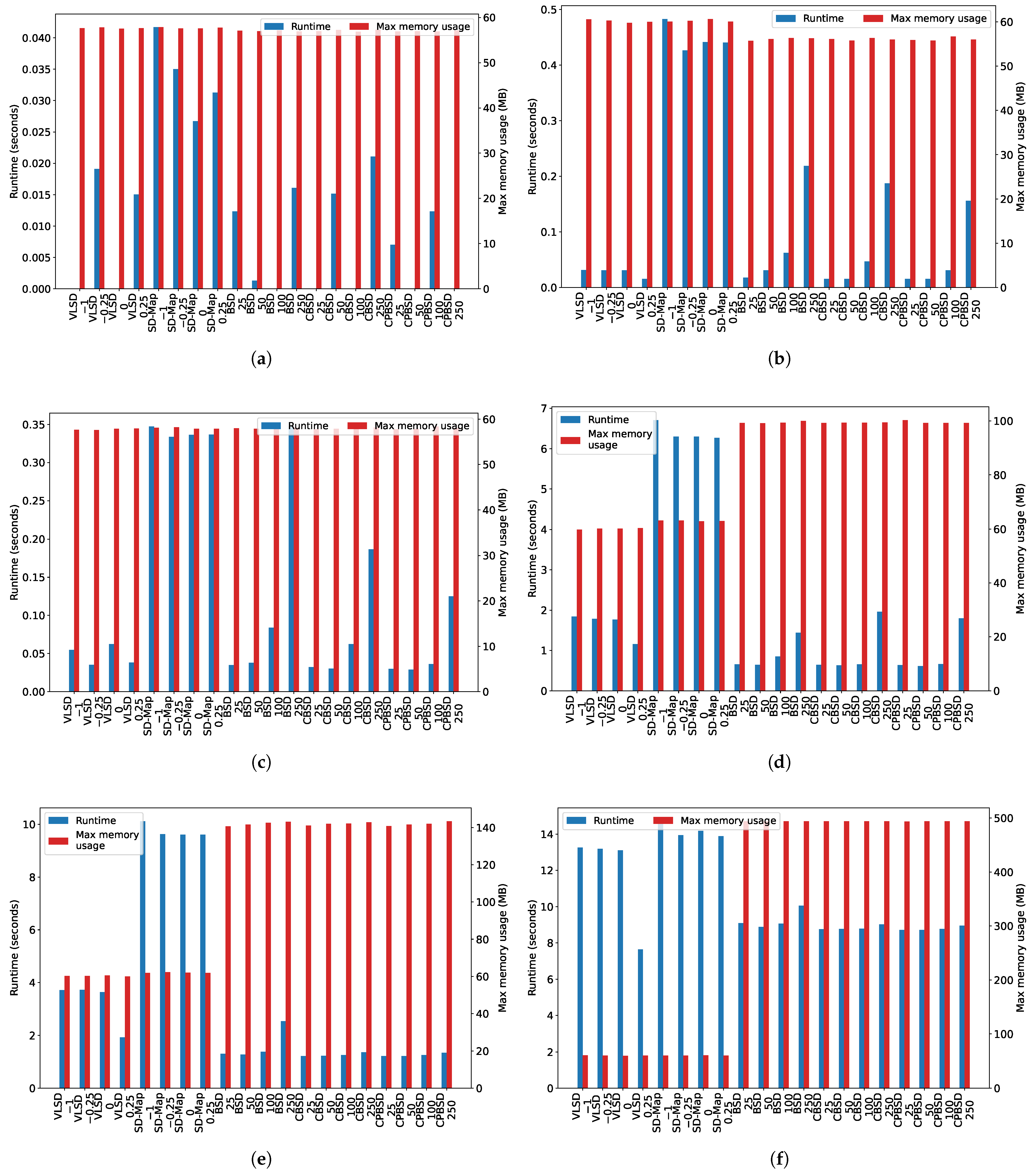
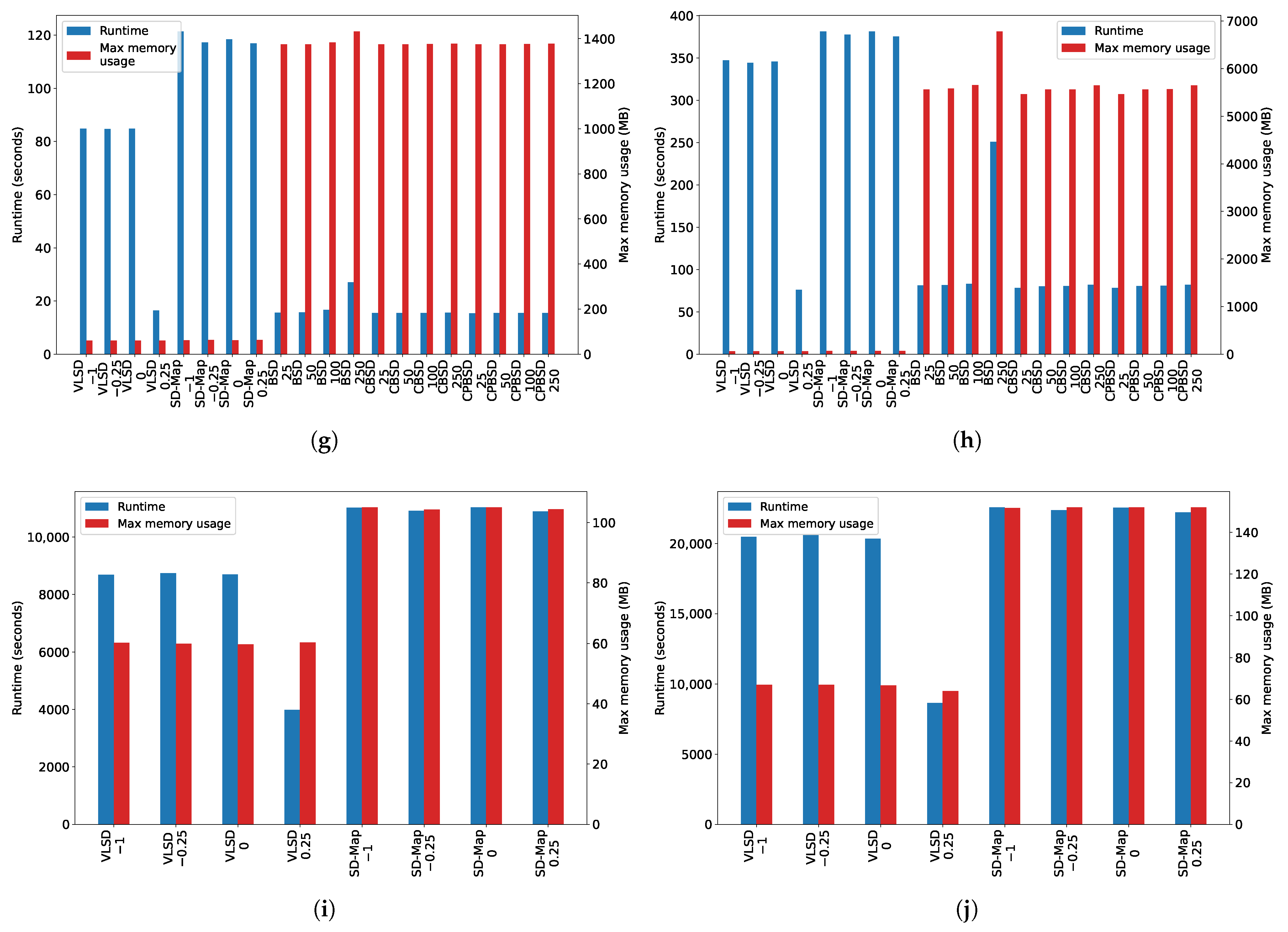
Focusing on the runtime of the VLSD and SD-Map algorithms,
Figure 8 shows that (1) there are significant differences among the executions of the VLSD algorithm (the higher the threshold, the less the time); (2) there are no significant difference between any of the execution of the SD-Map algorithm (i.e., using different threshold values), because that algorithm does not use a pruning based on optimistic estimate, and the complete search space is, therefore, always explored; and (3) although both algorithms have an exponential trend, VLSD runtime is, in general, less than SD-Map runtime. Finally,
Figure 9 also confirms these statements.
On the other hand, considering the runtime of the VLSD, BSD, CBSD, and CPBSD algorithms,
Figure 8 shows that (1) there are significant differences when increasing the top-k parameter in the BSD algorithm, and (2) there are no significant differences when increasing top-k parameter in the CBSD and CPBSD algorithms. The BSD algorithm explores a larger search space than the CBSD and CPBSD algorithms, which include an additional pruning for closed and closed-on-the-positives subgroups. The search space, therefore, increases in a more moderate manner in the CBSD and CPBSD algorithms when increasing the value of the top-k parameter. It is for this reason that the runtime increment of the BSD algorithm when increasing the top-k parameter is more significant than that of the CBSD and CPBSD algorithms. It will also be observed that (1) when the VLSD algorithm explores all the search space, its runtime is significantly higher than the runtime of the BSD, CBSD, and CPBSD algorithms; and (2) when the VLSD algorithm does not explore all the search space, there are no significant differences among its runtimes.
Concerning the max memory usage of the VLSD and SD-Map algorithms,
Figure 8 shows that (1) there are no significant differences among the executions of the VLSD algorithm, because its design and the utilization of the equivalence class exploration strategy make it extremely efficient and, although the complete search space may not explored in all cases, the memory usage is, in general, always reduced; (2) there are no significant differences among any of the executions of the SD-Map algorithm (i.e., using different threshold values), because the complete search space is always stored in the FPTree data structure, and (3) there are significant differences between both algorithms (as will be clearly noted in
Figure 8i,j). Finally,
Figure 10 confirms these statements, because it shows that the mean of the max memory usage of all datasets for each quality threshold value is always more than 20% larger when using the SD-Map algorithm.
Comparing the max memory usage of the VLSD, BSD, CBSD, and CPBSD algorithms,
Figure 8 shows the same behavior for BSD, CBSD, and CPBSD algorithms and for the same reasons as in the previous case. Additionally, note that, in general, these algorithms consume significantly more memory than the VLSD and SD-Map algorithms, and it is for this reason that it was impossible to execute them with the last two datasets.
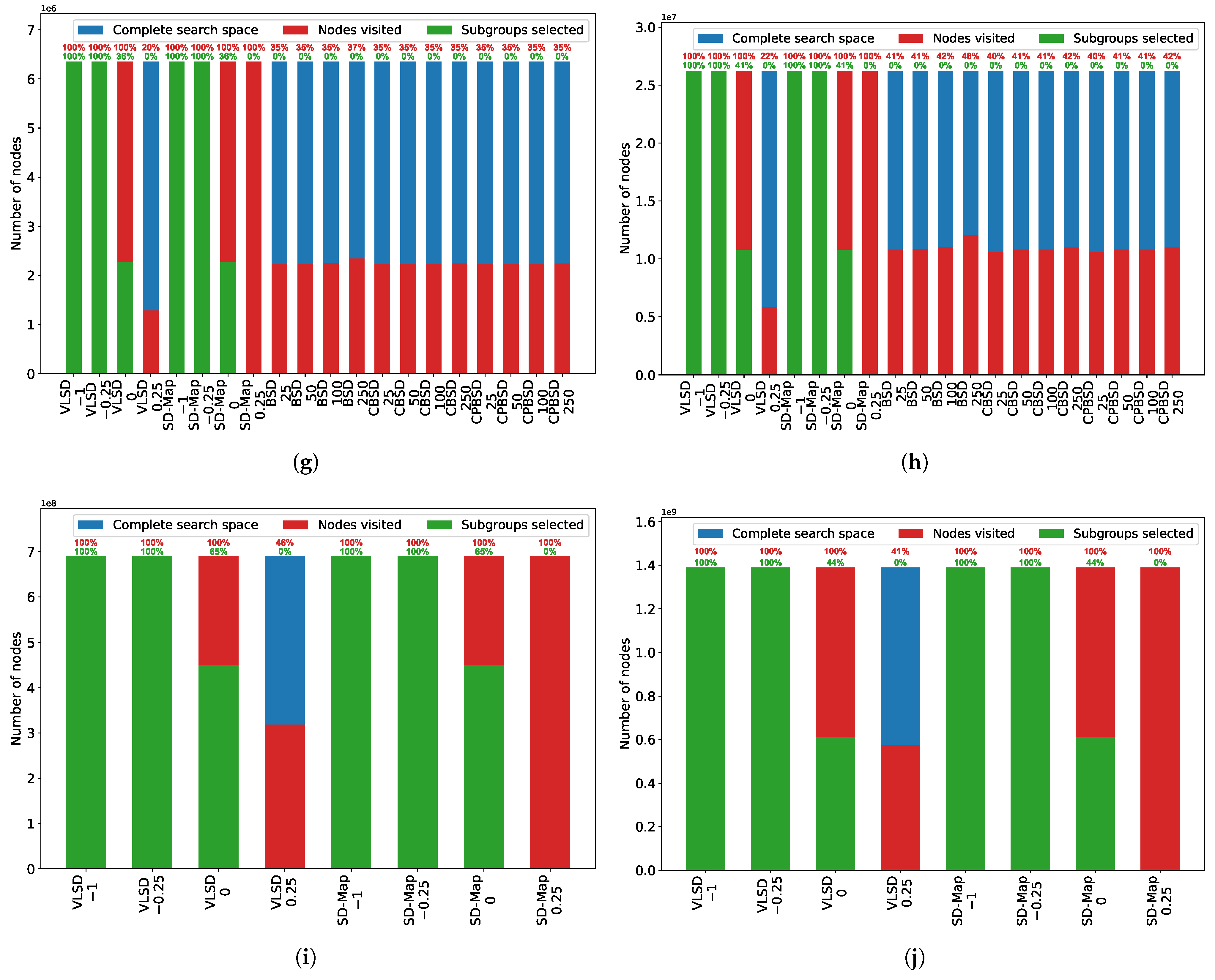
When focusing on the search space nodes of the VLSD algorithm (
Figure 11), it is important to state that, although it may not explore certain regions in the search space that have less quality owing to the utilization of the pruning based on optimistic estimate, this algorithm guarantees that the best subgroups will be found, because it is exhaustive.
Regarding the search space nodes of the VLSD and SD-Map algorithms,
Figure 11 shows that, first, the same subgroups are always generated for each dataset and for each threshold value. This proves that VLSD has been correctly designed and implemented, because it generates the same subgroups as the SD-Map, which is an exhaustive algorithm without optimistic estimate. Moreover, this figure also demonstrates the utilization of a pruning based on optimistic estimate, because, while the VLSD algorithm does not always explore the complete search space, the SD-Map algorithm always does so. Note that the VLSD algorithm explores fewer nodes when the threshold value is higher.
On the other hand, when comparing the search space nodes of the VLSD, BSD, CBSD, and CPBSD algorithms,
Figure 11 shows that the BSD, CBSD, and CPBSD algorithms (1) do not explore the complete search space, because they use a pruning based on optimistic estimate; and (2) select significantly fewer subgroups than the VLSD and SD-Map algorithms, because they implement an additional pruning based on relevant subgroups (and, moreover, CBSD and CPBSD also implement another pruning based on closed subgroups and closed-on-the-positives subgroups, respectively).
It is necessary to state that the bitsets used by the VLSD algorithm are different from those employed by the BSD, CBSD and CPBSD algorithms. While our algorithm considers all the dataset instances in both bitsets, the others use bitsets of different sizes.
In summary, when comparing the VLSD and SD-Map algorithms, it will be noted that the utilization of a pruning based on optimistic estimate by the VLSD algorithm has an evident impact. It will also be noted that, overall, this pruning strategy allows the VLSD algorithm to spend less time, consume less memory, and visit fewer nodes; all of this while remaining exhaustive and generating the same subgroups. Additionally, when comparing the VLSD, BSD, CBSD, and CPBSD algorithms, it will be noted that the last three algorithms are at a clear disadvantage with respect to the VLSD algorithm as regards the max memory usage. However, it will also be noted that, overall, the BSD, CBSD, and CPBSD algorithms spend less time and select less nodes owing to the pruning based on optimistic estimate, relevant subgroups, closed subgroups, and closed-on-the-positives subgroups.
6. Conclusions
This research was carried out in order to design and implement a new exhaustive Subgroup Discovery (SD) algorithm that would be more efficient than the state-of-the-art algorithms. We have proposed the VLSD algorithm, along with a new data structure denominated as a vertical list. This algorithm is based on the equivalence class exploration strategy and uses a pruning based on optimistic estimate.
Note that, although all these concepts already appear in the literature separately, this is the first time that they are used, implemented, and validated together.
Some existing SD algorithms, such as SD-Map or BSD, have adapted and used classical data structures, such as FPTree or Bitsets. Our algorithm uses a vertical list data structure, which represents both a subgroup and the dataset instances in which it appears. Moreover, it provides an easy and efficient computation of the subgroup refinements. The VLSD algorithm is also easily parallelizable owing to the utilization of the equivalence class exploration strategy, along with the aforementioned data structure.
Our experiments were carried out using a collection of standard, well-known, and popular datasets from the literature, and analyzed certain metrics, such as runtime, max memory usage, subgroups selected, and nodes visited. They confirmed that, overall, our approach is more efficient than the other algorithms considered.
Additionally, as an example of practical implications, this algorithm could be applied to certain specific domains, e.g., medical research or patient phenotyping.
Future research could continue and extend the algorithm in different ways. First, certain modifications could be made in order to avoid the need to extract all the subgroups explored (e.g., extracting only the top-k subgroups). Finally, some other pruning strategies could be added in order to make the VLSD algorithm even more efficient (e.g., closed subgroups or closed-on-the-positives subgroups).


 ,
, 


