Article

Parallel Algorithm for Solving Overdetermined Systems of Linear Equations, Taking into Account Round-Off Errors

by
Dmitry Lukyanenko
Department of Mathematics, Faculty of Physics, Lomonosov Moscow State University, Moscow 119991, Russia
Algorithms 2023, 16(5), 242; https://doi.org/10.3390/a16050242
Submission received: 9 April 2023 / Revised: 30 April 2023 / Accepted: 3 May 2023 / Published: 7 May 2023
(This article belongs to the Collection Parallel and Distributed Computing: Algorithms and Applications)

Abstract

:
The paper proposes a parallel algorithm for solving large overdetermined systems of linear algebraic equations with a dense matrix. This algorithm is based on the use of a modification of the conjugate gradient method, which is able to take into account rounding errors accumulated during calculations when making a decision to terminate the iterative process. The parallel algorithm is constructed in such a way that it takes into account the capabilities of the message passing interface (MPI) parallel programming technology, which is used for the software implementation of the proposed algorithm. The programming examples are shown using the Python programming language and the mpi4py package, but all programs are built in such a way that they can be easily rewritten using the C/C++/Fortran programming languages. The advantage of using the modern MPI-4.0 standard is demonstrated.
MSC:
68W10; 65F10; 65F20; 65F30

Graphical Abstract

1. Introduction

When solving many applied problems, it often becomes necessary to solve systems of linear algebraic equations of the form
A x = b .
Here, in the general case, A is a dense rectangular matrix of dimension M × N ( M N ), and b is a column vector with M components. The problem is to find out a vector x solving System (1).
When solving real applied problems, the components of the vector b on the right side of System (1) are usually measured experimentally. Therefore, due to the presence of experimental errors, this system may not have a classical solution. However, the pseudo-solution given by the least squares method is always obtained and it is the best approximation:
x = argmin x R N f ( x ) , where f ( x ) = A x b 2 2 .
The element realizing the minimum of Functional (2) can be found by solving the system of normal equations
A T A x = A T b .
In the most common case, when the matrix A is nondegenerate, System (3) can be solved using direct methods for solving systems of linear algebraic equations with a square matrix (see, for example, [1]).
Note that the matrix A T A of System (3) has dimension N × N . As a consequence, the implementation of direct solution methods in the case of an arbitrary matrix A requires O ( M N 2 ) operations: ( 2 M 1 ) N 2 operations to determine the matrix of System (3), ( 2 M 1 ) N operations to determine the right hand side, and O ( N 3 ) operations to implement the direct method of solving System (3). Therefore, for large values of M and N, the quality of the solution can be critically affected by rounding errors accumulating during the execution of these M N 2 operations.
In this regard, in practice, one often searches for an element that implements the minimum of Functional (2), not by solving a system of normal Equations (3), but by using gradient methods to minimize Functional (2) itself. These methods are iterative: they start from an arbitrary initial approximation for the solution and, at each iteration, find the next better approximation for the desired solution. When calculating without errors for an infinite number of iterations, such methods converge to the element x, which realizes the minimum of Functional (2).
Given that the problem (1) is linear, the most efficient gradient method for solving it is the conjugate gradient method (see, for example, [2,3,4]). This method, in the case of exact calculations, is able to find an element that implements the minimum of Functional (2) in exactly N iterations, each of which requires O ( M N ) operations. However, taking into account the fact that when solving practical problems, all calculations are performed only approximately (due to the presence of rounding errors), the statement about the possibility of minimizing the functional in exactly N iterations turns out to be incorrect. In practice, the following three situations are possible.
1.
Starting from some iteration, the number of which is less than N, the value of the minimized functional becomes comparable to the background of rounding errors. This means that all subsequent iterations are meaningless and the iterative process can be stopped, because the value of the functional will not decrease at subsequent iterations. Knowing such an iteration number makes it possible to interrupt calculations and save computational resources by finding an approximate solution by performing a much smaller number of operations compared to direct solution methods.
2.
In the first case, it is also possible that the execution of the full set of N iterations leads to “destruction” of the numerical solution. Thus, the possibility of early termination of the iterative process can be especially useful in solving applied problems. The implementation of this possibility in practice not only saves computational resources, but also makes it possible to find an adequate approximate solution.
3.
Due to the influence of rounding errors on the accuracy of determining the minimization directions and steps along them, after performing N iterations, the value of the minimized functional remains sufficiently large. This means that the approximate solution found after N iterations can be refined further if the iterative process is continued. In this case, the iterative process must be continued until the value of the functional reaches the background of rounding errors.
In other words, if in practice the “classic” criterion for stopping the iterative process in the conjugate gradient method is used (by a fixed number of iterations equal to N), then, in the first case, an approximate solution will be found, but excessive computational resources will be spent on its search; in the second case, the approximate solution will not be found at all; in the third case, a very rough approximate solution will be found, which can still be refined.
Thus, when solving many applied problems, the question of the possibility of developing such a criterion for terminating the iterative process in the conjugate gradient method, which would be able to take into account rounding errors accumulating in the process of calculations, is extremely important. Much work has been devoted to similar issues (see, for example, [5,6,7,8,9,10,11,12,13,14,15,16,17,18,19,20,21,22]). However, in the opinion of the author, it was in paper [23] that a rather detailed answer was given precisely to the question posed above. In this work, an algorithm was formulated that, in practice, allows for successfully solving all three of the above problem situations.
However, in work [23], the question of the ways of effective software implementation of the proposed algorithm was not considered. This issue is also extremely important. This is due to the fact that in order to solve many real systems of linear algebraic equations, it is necessary to use supercomputer (cluster) systems with many computing nodes. If such a supercomputer system is a multiprocessor system with distributed memory, then to organize the interaction of various computing nodes the message passing interface (MPI) message passing technology is usually used. At the same time, the efficiency of parallel software implementation is affected by the overhead costs for the interaction of computing nodes through the use of a communication network and the transmission of messages through it. Compared to the “classical” algorithm, the algorithm proposed in paper [23] has a lot of additional relatively small calculations, the execution of which on many computing nodes can generate a significant increase in overhead costs for the interaction of computing nodes [24,25,26]. That is, a fairly common problem in solving real applied problems may arise: the algorithm seems “good”, but its application to solving real applied problems is inefficient. However, the algorithm from [23] was designed in such a way that it allows for a fairly efficient parallel software implementation. Therefore, the purpose of this work is to demonstrate how the algorithm proposed in [23] can be effectively parallelized using the MPI parallel programming technology and using the MPI+OpenMP(+CUDA) parallel programming technologies. Thus, the novelty of this work lies in the development of an efficient parallel software implementation of the algorithm using the advantages of modern parallel programming technologies (MPI-4.0 standard of 2021).
The structure of this work is as follows. Section 2 describes the sequential algorithm from [23] and its software implementation. Section 3 describes parallel algorithms for implementing some basic linear algebra operations that will be used to construct a parallel version of the algorithm under consideration. Section 4 describes various approaches to constructing a parallel version of an algorithm and its software implementation, taking into account the capabilities of various MPI standards. Section 5 provides some tests of the proposed software implementations for the presence of strong and weak scalability and also gives recommendations for their use in computing on large parallel systems.

2. Sequential Algorithm and Its Software Implementation

For the sake of integrity of the presentation of the material, let us first recall (see Section 2.1) one of the classical implementations of the conjugate gradient method for solving System (1). This version of the conjugate gradient method was taken as the basis for the algorithm considered in [23] (see Section 2.2), the parallel version of which is the main subject of discussion of this work.

2.1. Classical Implementation of the Conjugate Gradient Method

The vector x with N components, which is a solution (pseudo-solution) of System (1), can be found using the following iterative algorithm that constructs the sequence x ( s ) . We set p ( 0 ) = 0 , s = 1 , and an arbitrary initial approximation x ( 1 ) . Then we execute the following sequence of actions N times:
r ( s ) = A T A x ( s ) b , if s = 1 , r ( s 1 ) q ( s 1 ) p ( s 1 ) , q ( s 1 ) , if s 2 , p ( s ) = p ( s 1 ) + r ( s ) r ( s ) , r ( s ) , q ( s ) = A T A p ( s ) , x ( s + 1 ) = x ( s ) p ( s ) p ( s ) , q ( s ) , s = s + 1 .
As a result, after N steps, the vector x r e s = x ( N + 1 ) will be a solution (pseudo-solution) of System (1), based on the assumption that all calculations are done exactly [2].
Remark 1. 
If we do not use the recurrent notation and calculate the residual r ( s ) at each iteration in the same way as at the first iteration ( s = 1 ), then the number of arithmetic operations required to complete the iteration process will double. When solving “large” problems, this is the motivation for using the recursive form of the conjugate gradient method.
This algorithm can be written as the following pseudocode (see Algorithm 1).
Algorithm 1: Pseudocode for a sequential version of the “classical” algorithm
Algorithms 16 00242 i001
    The Python code for the function that implements the conjugate gradient method for solving System (1) will have a fairly compact form (see Listing 1).
Listing 1. The Python code for a sequential version of the “classical” algorithm.
  •     def conjugate_gradient_method(A, b, x) :
  •         s = 1
  •         p = zeros(size(x))
  •         while s <= N :
  •             if s == 1 :
  •                         r = dot(A.T, dot(A,x) - b)
  •             else :
  •                         r = r - q/dot(p, q)
  •             p = p + r/dot(r, r)
  •             q = dot(A.T, dot(A, p))
  •             x = x - p/dot(p,q)
  •             s = s + 1
  •         return x
It is assumed that the standard package numpy is used for calculations. As a consequence, this seemingly sequential software implementation of the algorithm actually contains parallel computing. This is due to the peculiarity of the function dot() used for basic calculations from the package numpy. This function is implemented in the C++ programming language and automatically uses multithreading in calculations if the program is running on a multi-core processor—all processor cores are used through the use of OpenMP parallel programming technology.

2.2. Improved Implementation of the Conjugate Gradient Method

In work [23], a modification of the above conjugate gradient method was proposed, which takes into account rounding errors accumulated during of calculations when making a decision to terminate the iterative process.
We set p ( 0 ) = 0 , s = 1 , and an arbitrary initial approximation x ( 1 ) . Then we repeatedly perform the following sequence of actions:
r ( s ) = A T A x ( s ) b , if s = 1 , r ( s 1 ) q ( s 1 ) p ( s 1 ) , q ( s 1 ) , if s 2 , σ r ( s ) 2 = A T 2 A 2 x 2 + b 2 , if s = 1 , σ r ( s 1 ) 2 + ( q ( s 1 ) ) 2 p ( s 1 ) , q ( s 1 ) 2 , if s 2 , if Δ 2 n = 1 N σ r ( s ) 2 n r ( s ) 2 2 1 , then   the   iterative   process   interrupted ,   and   x ( s ) is   the   solution , p ( s ) = p ( s 1 ) + r ( s ) r ( s ) , r ( s ) , q ( s ) = A T A p ( s ) , x ( s + 1 ) = x ( s ) p ( s ) p ( s ) , q ( s ) , s = s + 1 .
Here, 2 is Hadamard power, that is, element-wise raising of a vector/matrix to the second power, Δ —relative rounding error. For half-precision calculation (float16) Δ = 10 3.3 , for single precision calculation (float32) Δ = 10 7.6 , for calculation with double precision (float64) Δ = 10 16.3 , and for calculating with quadruple precision Δ = 10 34.0 .
This algorithm can be written as the following pseudocode (see Algorithm 2). In this algorithm, the lines highlighted in red correspond to the actions that must be performed in order to implement the improved criterion for terminating the iterative process. If these lines are removed and the condition T r u e is changed to s N , then we get the “classical” implementation of the conjugate gradient method for solving System (1).
The Python code for the function that implements the conjugate gradient method for solving System (1) with the improved iterative process termination criterion is presented at Listing 2.
This software implementation contains the following features:
1.
The function returns (1) the array x that contains the solution of System (1) found by the improved Algorithm 2, (2) the number of iterations s that needed to be done by the algorithm to find an approximate solution, (3) the array x_classic, which contains the solution found using the “classical” Algorithm 1 (this array contains such a solution only if the number of iterations performed by the algorithm s N + 1 ).
2.
This implementation (and the corresponding pseudocode) takes into account that the result of each dot product is used twice, so the result of the dot product is stored in a separate variable.
3.
At the first iteration of the algorithm ( s = 1 ), the value of σ r 2 is calculated using the command
 sigma2_r = dot(A.T**2, dot(A**2, x**2) + b**2)
A feature of Python is that under the arrays A**2 and A.T**2, which contain the matrices A 2 and A T 2 , a separate memory space is allocated. This is very bad, because it is assumed that problem (1) is being solved with a huge matrix A.
Algorithm 2: Pseudocode for a sequential version of the improved algorithm
Algorithms 16 00242 i002
Listing 2. The Python code for a sequential version of the improved algorithm.
  •     def conjugate_gradient_method(A, b, x) :
  •         x_classic = None
  •         s = 1
  •         p = zeros(size(x))
  •         while True :
  •             if s == 1 :
  •                         r = dot(A.T, dot(A,x) - b)
  •                         sigma2_r = dot(A.T**2, dot(A**2, x**2) + b**2)
  •             else :
  •                 r = r - q/scalar_product_pq
  •                 sigma2_r = sigma2_r + q**2/scalar_product_pq**2
  •             scalar_product_rr = dot(r, r)
  •             delta = finfo(r.dtype).eps
  •             criterion = delta**2 * sum(sigma2_r)/scalar_product_rr
  •             if criterion >= 1 :
  •                         return x, s, x_classic
  •             p = p + r/scalar_product_rr
  •             q = dot(A.T, dot(A, p))
  •             scalar_product_pq = dot(p, q)
  •             x = x - p/scalar_product_pq
  •             s = s + 1
  •             if s == size(x) + 1 :
  •                         x_classic = x.copy()
Therefore, when solving real “large” problems, an array containing matrix A can take up a large part of the memory. As a result, there may not be enough space in memory for additional arrays.
This problem can be worked around in several ways.
In the first case, it is possible to issue the specified command as a separate function in the C/C++/Fortran programming language, using for calculations only the elements of the array in which matrix A is stored.
In the second case, it can be used a specially written function
  • sigma2_r = dot_special(A.T, dot_special(A,x**2,M,N)+b**2, N, M)
that uses “jit”-compilation using the package numba:
  • from numba import jit,prange
  •  
  • @jit(nopython=True, parallel=True)
  • def dot_special(A, x, M, N):
  •    b = empty(M)
  •    for m in prange(M):
  •      b[m] = 0.
  •      for n in range(N):
  •        b[m] = b[m] + A[m, n]**2*x[n]
  •    return b
However, in order not to overload the software implementation of the algorithm with such technical features, we will choose the third way.
In the third case, we can neglect the accumulating machine rounding error at the first iteration and set at the first iteration ( s = 1 ) σ r 2 = 0 :
  • sigma2_r = zeros(N)
Further, in all software implementations, we will choose the third way, as numerous numerical experiments have shown that when solving real applied problems, the accumulating machine rounding error at the first iteration ( s = 1 ) can be neglected. However, if desired, the corresponding programs can be easily improved to take into account the rounding error at the first iteration.

2.3. An Example of How the Algorithm Works

To demonstrate the capabilities of the algorithm proposed in [23], we will use (1) a matrix A of dimension M × N with elements generated as random variables with a uniform distribution in the range [ 0 , 1 ] , (2) model solution x m o d e l —a vector of dimension N, whose elements correspond to uniformly distributed values of the sine on the interval [ 0 , 2 π ] :
x n m o d e l = sin 2 π ( n 1 ) N 1 , n 1 , N ¯ .
Given matrix A and model solution x m o d e l , first calculate the right side b: b = A x m o d e l . To solve System (1) with this matrix A and the right side b, we apply the considered implementation of the conjugate gradient method with an improved criterion for terminating the iterative process. We will perform all calculations with double precision (float64), i.e., Δ 10 16 .
Remark 2. 
Note that all subsequent results may slightly differ in details during reproduction, as A matrix is randomly assigned.
Figure 1 shows an approximate solution—vector x r e s for M = 1000 , N = 1000 . The algorithm needed to complete s = 2476 iterations, which is significantly more than s = 1000 in the case of using the “classical” implementation of the conjugate gradient method to solve System (1). However, it is perfectly clear that the approximate solution found by the classical method (marked in red on the graph) is quite different from the exact one (sine), even visually. At the same time, the solution found using the improved algorithm does not visually differ from the exact solution.
If, however, calculations are made for M = 3000 , N = 1000 , then the approximate solution, which does not visually differ from the exact model solution, will be found in just s = 75 iterations, which is fewer than the 1000 iterations that would be required to find a solution using the classical algorithm.
Thus, this example clearly demonstrates that the algorithm proposed in [23], depending on the situation, allows for both stopping the iteration process ahead of schedule (thus saving computational resources) and continuing the iteration process (thus obtaining a better approximation solution).

3. Approaches to Building a Parallel Algorithm and Its Software Implementation

This section will describe the main approaches that will be used to construct a parallel version of the considered algorithm and its subsequent software implementation. In this case, the capabilities of the MPI parallel programming technology will be taken into account.

3.1. Parallelizable Operations

In the considered implementation of the conjugate gradient method for solving Problem (1), all calculations fall on the following four operations.
1.
The scalar product of two vectors of dimension N.
This operation requires N multiplications and N 1 additions—for a total of 2 N 1 arithmetic operations. It is customary to denote 2 N 1 = O ( N 1 ) , which indicates the linear computational complexity of the scalar product operation.
2.
Multiplication of a matrix of dimension M × N by a vector of dimension N.
To obtain each element of the final vector, it is necessary to scalarly multiply the corresponding row of the A matrix by the multiplied vector. Such calculations must be carried out for each element of the vector, which is the result of multiplication. Thus, M · ( 2 N 1 ) arithmetic operations must be performed in total. In the case of a square matrix ( M = N ), there will be O ( N 2 ) of such operations, which indicates the quadratic computational complexity of the operation of multiplying a matrix by a vector.
3.
Multiplication of a transposed matrix of dimension N × M by a vector of dimension M.
The computational complexity of this operation is equivalent to the operation of multiplying a matrix by a vector.
4.
Addition of two vectors of dimension N.
This operation requires N additions. That is, the computational complexity of this operation is linear.
Next, the algorithms used to parallelize these operations are considered, which will be used to build a parallel version of Algorithm 2 and its software implementation.

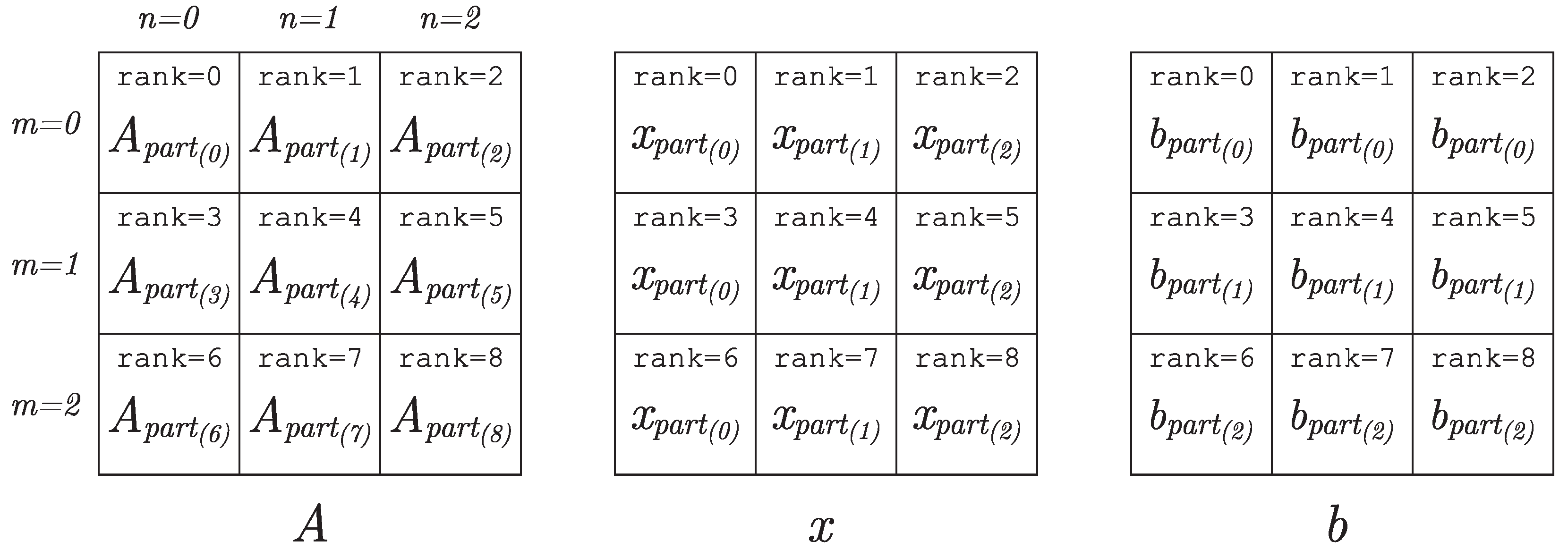
3.2. Distribution of Data by MPI Processes Participating in Computations

We will assume that the software implementation of the developed parallel algorithm will use the MPI parallel programming technology and run on the number of MPI processes equal to numprocs. All these processes will be included in the communicator comm ≡ MPI.COMM_WORLD, inside which they will have their number/identifier rank 0 , numprocs 1 ¯ .
Let us distribute all elements of the matrix A into blocks between the processes involved in the calculations using the two-dimensional division of the matrix into blocks (see Figure 2).
In this case, the number of splits along the vertical will be denoted as num_row (short for number of rows), and the number of splits along the horizontal—num_col (short for number of columns). As a result, matrix A of dimension M × N will be divided into parts A p a r t ( rank ) of dimension M p a r t ( m ) × N p a r t ( n ) . Here, the process number rank is related to indices m and n as follows:
m = rank num _ col , n = rank rank num _ col · num _ col .
Remark 3. 
Let us immediately pay attention to the fact that the chosen indexing method assumes that all processes will take part in the calculations, that is, num_row·num_colnumprocs.
Note also that
m = 0 num _ row 1 M p a r t ( m ) = M , n = 0 num _ col 1 N p a r t ( n ) = N .
Thus, it is assumed that each MPI process contains the array A_part, which contains one of the parts A p a r t ( · ) of matrix A. In addition, each process contains arrays x_part and b_part, which contain one of the parts x p a r t ( · ) and b p a r t ( · ) of vectors x and b, respectively. The storage structure of the vectors x and b on different processes is also shown in Figure 2. It is clearly seen that the part x p a r t ( n ) of the vector x for a fixed index n is stored in all cells of the process grid column with index n. Similarly, the part b p a r t ( m ) of vector b for a fixed index m is stored in all cells of the process grid row with index m.

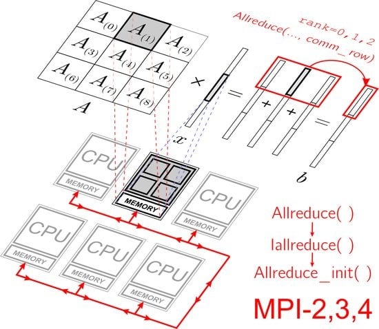
3.3. Parallel Algorithm for Matrix–Vector Multiplication in the Case of Two-Dimensional Division of the Matrix into Blocks

The terms that arise when calculating the product of a matrix and a vector can be divided into groups as follows (we give an example corresponding to Figure 3, when only nine MPI processes are involved in the calculations).
A x = A p a r t ( 0 ) A p a r t ( 1 ) A p a r t ( 2 ) A p a r t ( 3 ) A p a r t ( 4 ) A p a r t ( 5 ) A p a r t ( 6 ) A p a r t ( 7 ) A p a r t ( 8 ) x p a r t ( 0 ) x p a r t ( 1 ) x p a r t ( 2 ) = = A p a r t ( 0 ) x p a r t ( 0 ) + A p a r t ( 1 ) x p a r t ( 1 ) + A p a r t ( 2 ) x p a r t ( 2 ) A p a r t ( 3 ) x p a r t ( 0 ) + A p a r t ( 4 ) x p a r t ( 1 ) + A p a r t ( 5 ) x p a r t ( 2 ) A p a r t ( 6 ) x p a r t ( 0 ) + A p a r t ( 7 ) x p a r t ( 1 ) + A p a r t ( 8 ) x p a r t ( 2 ) = = A p a r t ( 0 ) x p a r t ( 0 ) A p a r t ( 3 ) x p a r t ( 0 ) A p a r t ( 6 ) x p a r t ( 0 ) + A p a r t ( 1 ) x p a r t ( 1 ) A p a r t ( 4 ) x p a r t ( 1 ) A p a r t ( 7 ) x p a r t ( 1 ) + A p a r t ( 2 ) x p a r t ( 2 ) A p a r t ( 5 ) x p a r t ( 2 ) A p a r t ( 8 ) x p a r t ( 2 ) = = b p a r t _ t e m p ( 0 , 0 ) b p a r t _ t e m p ( 1 , 0 ) b p a r t _ t e m p ( 2 , 0 ) + b p a r t _ t e m p ( 0 , 1 ) b p a r t _ t e m p ( 1 , 1 ) b p a r t _ t e m p ( 2 , 1 ) + b p a r t _ t e m p ( 0 , 2 ) b p a r t _ t e m p ( 1 , 2 ) b p a r t _ t e m p ( 2 , 2 ) = = b t e m p ( 0 ) + b t e m p ( 1 ) + b t e m p ( 2 ) = b p a r t ( 0 ) b p a r t ( 1 ) b p a r t ( 2 ) = b .
This form of representation of the multiplication of a matrix by a vector was chosen in order to clearly show that the vector x (it is assumed that it consists of N elements) does not need to be stored entirely on each process. Each process needs only its own part x p a r t ( n ) of this vector with N p a r t ( n ) elements, where n 0 , num _ col 1 ¯ .
Then, each process participating in the calculations will perform the operation of multiplying its part A p a r t ( rank ) of matrix A by its part x p a r t ( n ) of vector x. As a result of this operation, the vector b p a r t _ t e m p ( m , n ) will be calculated, which will be one of the terms of the part b p a r t ( m ) of the final vector b. Each process participating in the calculation can perform this action independently of other processes while operating only with the data that are located in the memory of this process. These calculation actions can be implemented in parallel. Then, the corresponding summands b p a r t _ t e m p ( m , n ) along each line of the process grid (i.e., index m is fixed) must be collected (due to message exchange between processes) at least on one process and summed up.
Thus, this parallel algorithm (taking into account the two-dimensional division of matrix A into blocks) contains the following features.
1.
Each process should store not the whole vector x, but only a part x p a r t ( n ) of this vector. The vector x p a r t ( n ) will have to be sent not to all processes of the comm communicator, but only to a part of the processes of this communicator—to the processes of the column with index n of the process grid. In this case, the transfer of data among the processes of each column of the process grid can be organized in parallel with the transfer of data among the processes of other columns of the grid of processes, which will give a gain in time.
2.
When calculating part b p a r t ( m ) of the final vector b, it is necessary to exchange messages not to all processes of the comm communicator, but only to part of the processes of this communicator—to the processes of the line with index m of the introduced grid of processes. In this case, the data transfer along each line of the process grid can be organized in parallel with the transfer of data among the processes of other lines of the process grid, which will also give a gain in time.
Let us now describe some features of the software implementation of this algorithm, taking into account the capabilities of the MPI parallel programming technology.
As is known, message exchange between processes for the aforementioned algorithm, organized using the MPI functions Send() and Recv(), is possible, but inefficient. It is much more efficient to use the MPI functions of the collective interaction of processes. However, such functions must be called on all processes of the communicator. At the moment, we are working only with the communicator comm, which, in addition to the processes that we want to use (processes from a separate column or row of the process grid), also contains other processes that will not interact with one another. Thus, we come to the need to create additional communicators that will contain only those groups of processes within which we want to organize data exchange interactions using the functions of collective interaction of processes.
Such communicator groups can be created, for example, as follows.
  • comm_col = comm.Split(rank % num_col, rank)
  • comm_row = comm.Split(rank // num_col, rank)
Here, for example, the communicators comm_col are generated in the first line. Let us pay attention to the fact that it is the communicators (in the plural) that are generated, and not just one communicator. Let us give an explanatory example for the case of nine MPI processes (that is, numprocs = 9). The first argument of the Split() function is the color value, defined by us as rank % num_col, which, for processes with rank = 0, 1, 2, 3, 4, 5, 6, 7, 8, will be 0, 1, 2, 0, 1, 2, 0, 1, 2. Thus, three communicators will be created: the first one will include processes with the value color = 0, the second one—with the value color = 1, the third one—with the value color = 2. One can give a visual interpretation of such a grouping of processes—see Figure 2: if the processes of the communicator comm form a two-dimensional grid, then the processes of the communicators comm_col are columns of this two-dimensional grid of processes.
In this case, the object comm_col on each MPI process will contain information about different processes. For example, on processes with rank = 1, 4 of the communicator comm, the object comm_col will contain information about processes with rank = 1, 4, 7 of the communicator comm. And on a process with rank = 2 of the communicator comm, the object comm_col will contain information about processes with rank = 2, 5, 8 of the communicator comm.
Similarly, if the processes of the communicator comm form a two-dimensional grid, then the processes of communicators comm_row are rows of this two-dimensional grid of processes.
Thus, a parallel software implementation of matrix-vector multiplication can be presented in the following form:
  • b_part_temp = dot(A_part, x_part)
  • b_part = empty(M_part, dtype=float64)
  • comm_row.Allreduce([b_part_temp, M_part, MPI.DOUBLE],
  •                    [b_part, M_part, MPI.DOUBLE], op=MPI.SUM)
Note that the result of such a multiplication (vector b) will be stored on all processes in parts: a part b p a r t ( m ) of the vector b for a fixed index m will be stored in all cells of the process grid row with index m.
Remark 4. 
Recall that the message exchange time is proportional to log 2 numprocs , but the volume of transmitted messages is proportional to numprocs 1 / 2 in the case of a two-dimensional matrix division by blocks and is constant in the case of one-dimensional division of the matrix into blocks [1,27].

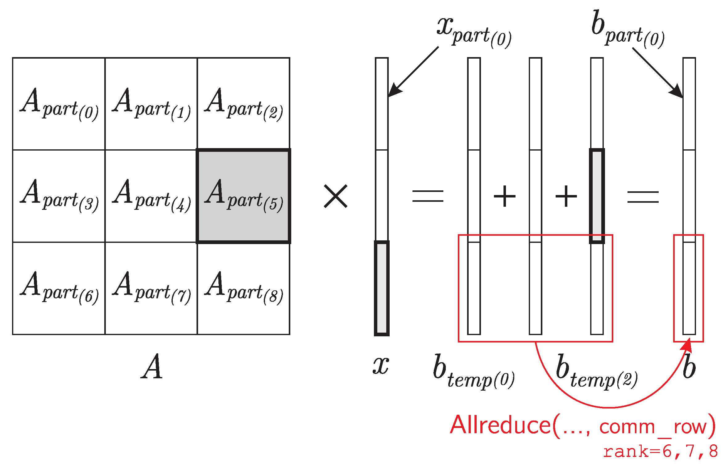
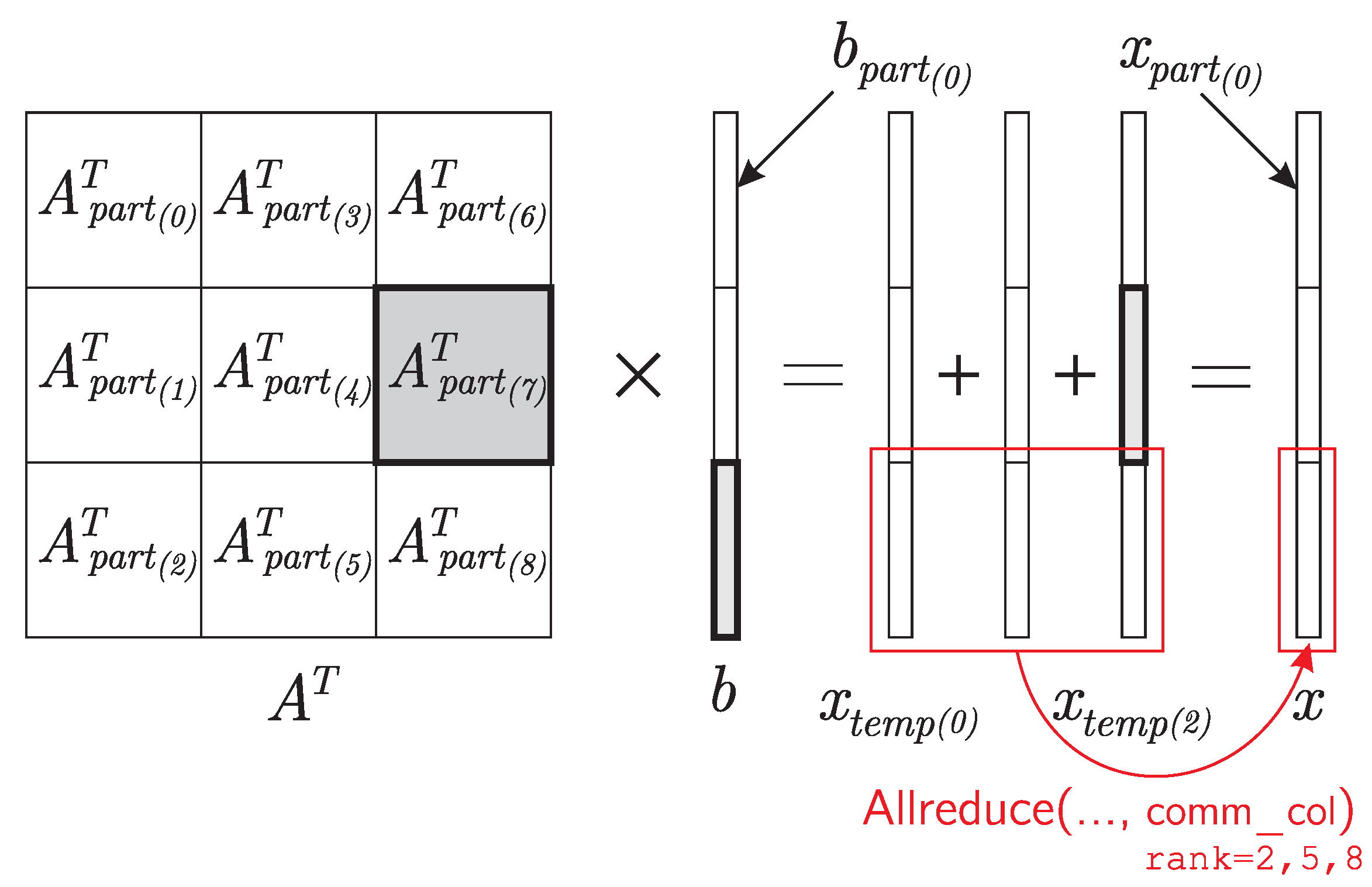
3.4. A Parallel Algorithm for Multiplying a Transposed Matrix by a Vector in the Case of Two-Dimensional Division of a Matrix into Blocks

The parallel algorithm for multiplying a transposed matrix by a vector in the case of a two-dimensional division of a matrix into blocks is quite similar to the algorithm considered in the previous section, and in a sense has symmetry with respect to it. Because we are interested in the multiplication of a transposed matrix by a vector in the context of the conjugate gradient method, we assume that system matrix A is stored over the processes of the grid of processes as shown in Figure 2. This is due to the fact that it is necessary to build an algorithm for multiplying matrix A T by a vector in such a way as to avoid creating additional arrays in memory for the transposed matrix. Indeed, when solving real applied problems, the total available memory on all processes may not be enough. We build algorithms for solving very large problems!
Therefore, the terms that arise when calculating the product of a transposed matrix by a vector can be divided into groups as follows (as in the previous section, we will give an example in which only nine MPI processes are involved in the calculations, see Figure 4):
A T b = A p a r t T ( 0 ) A p a r t T ( 3 ) A p a r t T ( 6 ) A p a r t T ( 1 ) A p a r t T ( 4 ) A p a r t T ( 7 ) A p a r t T ( 2 ) A p a r t T ( 5 ) A p a r t T ( 8 ) b p a r t ( 0 ) b p a r t ( 1 ) b p a r t ( 2 ) = = A p a r t T ( 0 ) b p a r t ( 0 ) + A p a r t T ( 3 ) b p a r t ( 1 ) + A p a r t T ( 6 ) b p a r t ( 2 ) A p a r t T ( 1 ) b p a r t ( 0 ) + A p a r t T ( 4 ) b p a r t ( 1 ) + A p a r t T ( 7 ) b p a r t ( 2 ) A p a r t T ( 2 ) b p a r t ( 0 ) + A p a r t T ( 5 ) b p a r t ( 1 ) + A p a r t T ( 8 ) b p a r t ( 2 ) = = A p a r t T ( 0 ) b p a r t ( 0 ) A p a r t T ( 1 ) b p a r t ( 0 ) A p a r t T ( 2 ) b p a r t ( 0 ) + A p a r t T ( 3 ) b p a r t ( 1 ) A p a r t T ( 4 ) b p a r t ( 1 ) A p a r t T ( 5 ) b p a r t ( 1 ) + A p a r t T ( 6 ) b p a r t ( 2 ) A p a r t T ( 7 ) b p a r t ( 2 ) A p a r t T ( 8 ) b p a r t ( 2 ) = = x p a r t _ t e m p ( 0 , 0 ) x p a r t _ t e m p ( 0 , 1 ) x p a r t _ t e m p ( 0 , 2 ) + x p a r t _ t e m p ( 1 , 0 ) x p a r t _ t e m p ( 1 , 1 ) x p a r t _ t e m p ( 1 , 2 ) + x p a r t _ t e m p ( 2 , 0 ) x p a r t _ t e m p ( 2 , 1 ) x p a r t _ t e m p ( 2 , 2 ) = = x t e m p ( 0 ) + x t e m p ( 1 ) + x t e m p ( 2 ) = x p a r t ( 0 ) x p a r t ( 1 ) x p a r t ( 2 ) = x .
Then, each process participating in the calculations will perform the operation of multiplying its part A p a r t T ( rank ) of matrix A T by its part b p a r t ( m ) of vector b. As a result of this operation, the vector x p a r t _ t e m p ( m , n ) will be calculated, which will be one of the terms of the part x p a r t ( n ) of the final vector x. Each process participating in the calculation can perform this action independently of other processes while operating only with the data that are located in the memory of this process. We are implementing these actions in parallel. Then, the corresponding summands x p a r t _ t e m p ( m , n ) along each column of the process grid (i.e., index n is fixed) must be collected (due to message exchange between processes) and measured on at least one process and summed up.
Thus, this parallel algorithm (taking into account the two-dimensional division of matrix A into blocks) contains the following features.
1.
Each process should store not the whole vector b, but only a part b p a r t ( m ) of this vector. The vector b p a r t ( m ) will have to be sent not to all the processes of the communicator comm, but only to a part of the processes of this communicator—to the processes of the row with index m of the process grid. In this case, the transfer of data among the processes of each row of the process grid can be organized in parallel with the transfer of data among the processes of other rows of the grid of processes, which will give a gain in time.
2.
When calculating the part x p a r t ( n ) of the final vector x, it is necessary to exchange messages not with all processes of the communicator comm, but only with part of the processes of this communicator—with the processes of the column with index n of the introduced grid of processes. In this case, the data transfer along each column of the process grid can be organized in parallel with the transfer of data among the processes of other columns of the process grid, which will also give a gain in time.
As you can clearly see, the parallel algorithm for multiplying a transposed matrix by a vector in the case of a two-dimensional division of a matrix into blocks has symmetry with respect to the parallel algorithm for multiplying a matrix by a vector, considered in the previous section. This algorithm is obtained from the previous one by replacing m n and “rows” ↔ “columns”. In this case, all actions are performed not with parts of the matrix A p a r t ( rank ) , but with their transposed parts A p a r t T ( rank ) . Thus, the software implementation of this algorithm will not differ much from the software implementation of the parallel algorithm for matrix–vector multiplication (including the need to work with additional communicators that will contain only those groups of processes among which we want to organize data exchange interactions using the functions of the collective process interactions).
Thus, a parallel software implementation of multiplying a transposed matrix by a vector (taking into account the fact that we operate with elements of the original non-transposed matrix) can be formalized in the following form:
  • x_part_temp = dot(A_part.T, b_part)
  • x_part = empty(N_part, dtype=float64)
  • comm_col.Allreduce([x_part_temp, N_part, MPI.DOUBLE],
  •                    [x_part, N_part, MPI.DOUBLE], op=MPI.SUM)
Note that the result of such a multiplication (vector x) will be stored on all processes in parts: part x p a r t ( n ) of the vector x for a fixed index n will be stored in all cells of the process grid column with index n.

3.5. Parallel Algorithm for Scalar Multiplication of Vectors

We will assume that the storage structure of the elements of vectors a and b (which each contain N elements) is the same as that of vector x (see Figure 2). We will denote such parts of vectors stored on different processes as a p a r t ( n ) and b p a r t ( n ) . Each such part will consist of N p a r t ( n ) elements. To simplify the presentation of the material, consider indexing for vectors stored in the first row of the process grid (with index m = 0 ). Therefore, n 0 , num _ col 1 ¯ .
The terms that arise when calculating the scalar product of vectors can be divided into groups as follows (we will also give an example in which only nine MPI processes are involved in the calculations):
( a , b ) = a p a r t ( 0 ) a p a r t ( 1 ) a p a r t ( 2 ) , b p a r t ( 0 ) b p a r t ( 1 ) b p a r t ( 2 ) = = a p a r t ( 0 ) , b p a r t ( 0 ) + a p a r t ( 1 ) , b p a r t ( 1 ) + a p a r t ( 2 ) , b p a r t ( 2 ) = = scalar _ product t e m p ( 0 ) + scalar _ product t e m p ( 1 ) + scalar _ product t e m p ( 2 ) = = scalar _ product .
Then, each process involved in the calculation will perform the operation ( a p a r t ( rank ) , b p a r t ( rank ) ) . As a result of this operation, one of the terms that make up the final scalar product will be calculated. Each process participating in the calculation can perform this action independently of other processes while operating only with the data that are located in the memory of this process. We implement these calculations in parallel. Then, the corresponding terms along each line of the process grid must be collected (due to the exchange of messages between processes) on at least one process and summed up.
Thus, the parallel software implementation of the scalar multiplication of vectors can be formalized in the following form:
  • scalar_product_temp = array(dot(r_part, r_part), dtype=float64)
  • scalar_product = array(0, dtype=float64)
  • comm_row.Allreduce([scalar_product_temp, 1, MPI.DOUBLE],
  •                    [scalar_product, 1, MPI.DOUBLE], op=MPI.SUM)
Note that the result of such a software implementation of scalar multiplication will be stored on all processes of the communicator comm.
Remark 5. 
The downside of this algorithm is that different groups of processes, each of which forms its own communicator comm_row, perform the same actions. However, this minus is insignificant in the context of the parallel implementation of the conjugate gradient method, in which this algorithm accounts for a negligibly small part of the calculations in the case of solving “large” problems.

4. Parallel Version of the Improved Algorithm and Its Software Implementation

This section describes various approaches to building a parallel version of Algorithm 2 and its software implementation. These approaches take into account the possibilities of various MPI standards. First (see Section 4.1), the “naive” approach to parallelization is described, which is based on the use of the MPI-2 standard. In this approach, additional time is spent on all additional operations related to accounting for rounding errors that accumulate in the process of calculations. Among other things, there are additional time costs for receiving/transmitting additional messages between processes that are required to organize additional calculations. Then (see Section 4.2), an approach to parallelization based on the MPI-3 standard is described. This approach, due to the use of non-blocking (asynchronous) messaging operations between processes, will make it possible to hide all additional calculations against the background of message exchange between processes in the main algorithm and hide additional message transfers against the background of calculations of the main algorithm. Due to this, all additional operations (calculations and message forwarding between MPI processes) do not require additional time. As a result, the efficiency of the software implementation of the improved algorithm does not differ from the efficiency of the software implementation of the classical algorithm. Then (see Section 4.3), comments are given regarding the use of the MPI-4 standard, which allows for increasing the efficiency of parallel software implementation through the use of persistent requests.

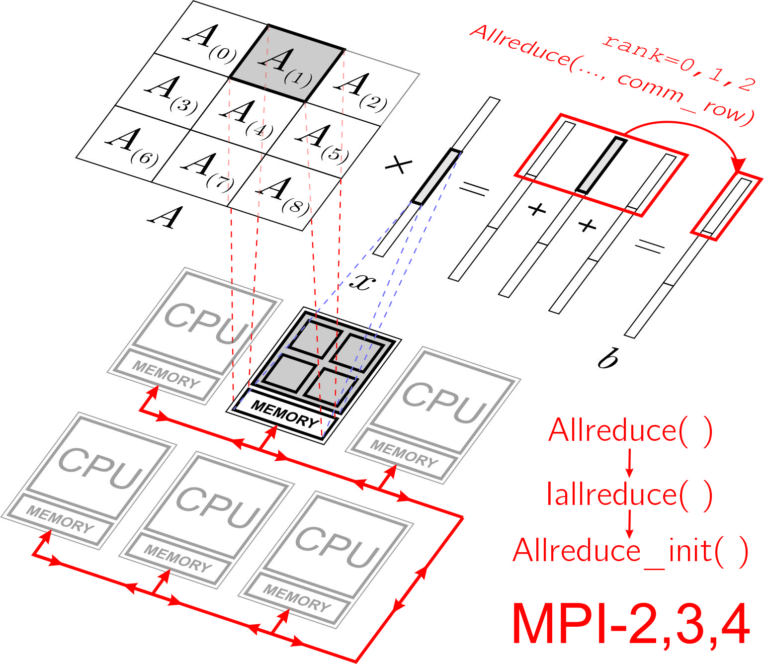
4.1. Taking into Account the Capabilities of the Standard MPI-2

A “naive” parallel version of Algorithm 2, which implements an improved implementation of the conjugate gradient method for solving System (1), can be written as the following pseudocode (see Algorithm 3). In this algorithm, the rows highlighted in red correspond to the actions that must be performed in order to implement the improved criterion for terminating the iterative process. If these lines are removed and the condition T r u e is changed to s N , then we get the classical implementation of the conjugate gradient method for solving System (1).
The software implementation of the function that implements Algorithm 3 for solving System (1) will look like Listing 3.
Similarly to the sequential version of the program, as a result of the operation of this function, each MPI process returns (1) an array x_part, which contains a part of the solution of System (1) found using the improved algorithm, and which, when combined with similar data from other processes will give an array x containing the complete solution of System (1); (2) the number of iterations s that the algorithm needed to do to find an approximate solution; and (3) the array x_classic_part, which contains a part of the solution found using the classical algorithm (this array contains such data only if the number of iterations performed by the algorithm is s N + 1 ).

4.2. Taking into Account the Capabilities of the Standard MPI-3

Taking into account the capabilities of the MPI-3 standard allows one, through the use of non-blocking (asynchronous) MPI operations (highlighted in the subsequent algorithm in blue), to perform additional calculations related to taking into account accumulated machine rounding errors, simultaneously with the transmission of the largest messages in the main algorithm, as well as forward additional messages against the background of the calculations of the main algorithm. The corresponding parallel algorithm can be written as the following pseudocode (see Algorithm 4).
The software implementation of the function that implements Algorithm 4 for solving System (1) will look like Listing 4.
Algorithm 3: Pseudocode for a (“naive”) parallel version of the improved algorithm
Algorithms 16 00242 i003
Listing 3. The Python code for a (“naive”) parallel version of the improved algorithm.
  • def conjugate_gradient_method(A_part, b_part, x_part,
  •                 comm_row, comm_col, N) :
  •  
  •     N_part = size(x_part);  M_part = size(b_part)
  •  
  •     x_classic_part = None
  •     delta = finfo(float64).eps
  •  
  •     s = 1
  •     p_part = zeros(N_part, dtype=float64)
  •  
  •     while True :
  •  
  •         if s == 1 :
  •             Ax_part_temp = dot(A_part, x_part)
  •             Ax_part = empty(M_part, dtype=float64)
  •             comm_row.Allreduce([Ax_part_temp, M_part, MPI.DOUBLE],
  •                                [Ax_part, M_part, MPI.DOUBLE],
  •                                op=MPI.SUM)
  •             b_part = Ax_part - b_part
  •             r_part_temp = dot(A_part.T, b_part)
  •             r_part = empty(N_part, dtype=float64)
  •             comm_col.Allreduce([r_part_temp, N_part, MPI.DOUBLE],
  •                                [r_part, N_part, MPI.DOUBLE],
  •                                op=MPI.SUM)
  •              sigma2_r_part = zeros(N_part, dtype=float64)
  •         else :
  •              r_part = r_part - q_part/scalar_product_pq
  •  
  •              sigma2_r_part = sigma2_r_part + \
  •                              q_part**2/scalar_product_pq**2
  •  
  •         scalar_product_temp = array(dot(r_part, r_part),
  •                                     dtype=float64)
  •         scalar_product_rr = array(0, dtype=float64)
  •         comm_row.Allreduce([scalar_product_temp, 1, MPI.DOUBLE],
  •                            [scalar_product_rr, 1, MPI.DOUBLE],
  •                            op=MPI.SUM)
  •  
  •         criterion_temp = array(delta**2*sum(sigma2_r_part)/
  •                                scalar_product_rr, dtype=float64)
  •         criterion = array(0, dtype=float64)
  •         comm_row.Allreduce([criterion_temp, 1, MPI.DOUBLE],
  •                            [criterion, 1, MPI.DOUBLE],
  •                            op=MPI.SUM)
  •         if criterion >= 1 :
  •             return x_part, s, x_classic_part
  •  
  •         p_part = p_part + r_part/scalar_product_rr
  •  
  •         Ap_part_temp = dot(A_part, p_part)
  •         Ap_part = empty(M_part, dtype=float64)
  •         comm_row.Allreduce([Ap_part_temp, M_part, MPI.DOUBLE],
  •                            [Ap_part, M_part, MPI.DOUBLE],
  •                            op=MPI.SUM)
  •         q_part_temp = dot(A_part.T, Ap_part)
  •         q_part = empty(N_part, dtype=float64)
  •         comm_col.Allreduce([q_part_temp, N_part, MPI.DOUBLE],
  •                            [q_part, N_part, MPI.DOUBLE],
  •                            op=MPI.SUM)
  •  
  •         scalar_product_temp = array(dot(p_part, q_part),
  •                                     dtype=float64)
  •         scalar_product_pq = array(0, dtype=float64)
  •         comm_row.Allreduce([scalar_product_temp, 1, MPI.DOUBLE],
  •                            [scalar_product_pq, 1, MPI.DOUBLE],
  •                            op=MPI.SUM)
  •         x_part = x_part - p_part/scalar_product_pq
  •  
  •         s = s + 1
  •         if s == N + 1 : x_classic_part = x_part.copy()
Algorithm 4: Pseudocode for an efficient parallel version of the improved algorithm
Algorithms 16 00242 i004
Listing 4. The Python code for an efficient parallel version of the improved algorithm.
  •     def conjugate_gradient_method(A_part, b_part, x_part,
  •                                                                 comm_row, comm_col, N) :
  •  
  •         N_part = size(x_part);  M_part = size(b_part)
  •  
  •         x_classic_part = None
  •         delta = finfo(float64).eps
  •  
  •         requests = [MPI.Request() for i in range(2)]
  •  
  •         s = 1
  •         p_part = zeros(N_part, dtype=float64)
  •  
  •         while True :
  •  
  •             if s == 1 :
  •                         Ax_part_temp = dot(A_part, x_part)
  •                         Ax_part = empty(M_part, dtype=float64)
  •                         comm_row.Allreduce([Ax_part_temp, M_part, MPI.DOUBLE],
  •                                                                 [Ax_part, M_part, MPI.DOUBLE],
  •                                                                 op=MPI.SUM)
  •                         b_part = Ax_part - b_part
  •                         r_part_temp = dot(A_part.T, b_part)
  •                         r_part = empty(N_part, dtype=float64)
  •                         comm_col.Allreduce([r_part_temp, N_part, MPI.DOUBLE],
  •                                                                 [r_part, N_part, MPI.DOUBLE],
  •                                                                 op=MPI.SUM)
  •  
  •                         sigma2_r_part = zeros(N_part, dtype=float64)
  •             else:
  •                         r_part = r_part - q_part/scalar_product_pq
  •  
  •             scalar_product_temp = array(dot(r_part, r_part),
  •                                                                         dtype=float64)
  •             scalar_product_rr = array(0, dtype=float64)
  •             comm_row.Allreduce([scalar_product_temp, 1, MPI.DOUBLE],
  •                                                     [scalar_product_rr, 1, MPI.DOUBLE],
  •                                                     op=MPI.SUM)
  •             p_part = p_part + r_part/scalar_product_rr
  •  
  •             Ap_part_temp = dot(A_part, p_part)
  •             Ap_part = empty(M_part, dtype=float64)
  •             requests[0] = comm_row.Iallreduce(
  •                                                                 [Ap_part_temp, M_part, MPI.DOUBLE],
  •                                                                 [Ap_part, M_part, MPI.DOUBLE],
  •                                                                 op=MPI.SUM)
  •  
  •             if s >= 2 :
  •                         sigma2_r_part =  sigma2_r_part + \
  •                                                             q_part**2/scalar_product_pq**2
  •             criterion_temp = array(delta**2*sum(sigma2_r_part)/
  •                                                                 scalar_product_rr, dtype=float64)
  •             criterion = array(0, dtype=float64)
  •             requests[1] = comm_row.Iallreduce(
  •                                                                 [criterion_temp, 1, MPI.DOUBLE],
  •                                                                 [criterion, 1, MPI.DOUBLE],
  •                                                                 op=MPI.SUM)
  •  
  •             MPI.Request.Wait(requests[0], status=None)
  •             q_part_temp = dot(A_part.T, Ap_part)
  •             q_part = empty(N_part, dtype=float64)
  •             comm_col.Allreduce([q_part_temp, N_part, MPI.DOUBLE],
  •                                                      [q_part, N_part, MPI.DOUBLE],
  •                                                      op=MPI.SUM)
  •  
  •             scalar_product_temp = array(dot(p_part, q_part),
  •                                                                        dtype=float64)
  •             scalar_product_pq = array(0, dtype=float64)
  •             comm_row.Allreduce([scalar_product_temp, 1, MPI.DOUBLE],
  •                                                     [scalar_product_pq, 1, MPI.DOUBLE],
  •                                                     op=MPI.SUM)
  •  
  •             MPI.Request.Wait(requests[1], status=None)
  •             if criterion >= 1 :
  •                         return x_part, s, x_classic_part
  •  
  •             x_part = x_part - p_part/scalar_product_pq
  •  
  •             s = s + 1
  •  
  •             if s == N + 1 :
  •                     x_classic_part = x_part.copy()

4.3. Taking into Account the Capabilities of the Standard MPI-4

The program implementation of Algorithm 4 contains collective operations between processes with the same argument list, which are executed in a loop. This means that it may be possible to optimize the communication by binding the list of communication arguments to a persistent communication request once and, then, repeatedly using the request to initiate and complete messages.
Changes in the software implementation will be fairly simple. The following sequence of changes must be made.
1.
Before the main loop while, it is necessary to form persistent communication request using MPI functions of the form request[] = Allreduce_init() for all functions of collective interaction of processes Allreduce() and Iallreduce() that occur inside the loop.
Remark 6. 
The arguments to these functions are numpy arrays, namely the fixed memory areas associated with these arrays. When initializing the persistent communication request, all data will be taken/written to these memory areas, which are fixed once when the corresponding persistent request is generated. Therefore, it is necessary to first allocate space in memory for all arrays that are arguments to these functions and, during subsequent calculations, ensure that the corresponding results of the calculations are stored in the correct memory areas.
2.
Inside the while loop, replace the MPI function Allreduce() with the sequence of MPI functions Start(request[]) “+” Wait(request[]).
3.
Inside the while loop, replace the MPI function Iallreduce() with the MPI function Start(request[]).
Corresponding software implementation of the function that implements Algorithm 4 for solving System (1) will look like Listing 5.
Listing 5. The Python code for an efficient parallel version of the improved algorithm with using the MPI-4.0 standart
  • def conjugate_gradient_method(A_part, b_part, x_part,
  •                                                                 comm_row, comm_col, N) :
  •  
  •     N_part = size(x_part);  M_part = size(b_part)
  •  
  •     x_classic_part = None
  •     delta = finfo(float64).eps
  •  
  •     requests = [MPI.Request() for i in range(5)]
  •  
  •     scalar_product_temp = empty(1, dtype=float64)
  •     scalar_product_rr = array(0, dtype=float64)
  •     scalar_product_pq = array(0, dtype=float64)
  •  
  •     Ap_part_temp = empty(M_part, dtype=float64)
  •     Ap_part = empty(M_part, dtype=float64)
  •  
  •     q_part_temp = empty(N_part, dtype=float64)
  •     q_part = empty(N_part, dtype=float64)
  •  
  •     criterion_temp = empty(1, dtype=float64)
  •     criterion = array(0, dtype=float64)
  •  
  •     requests[0] = comm_row.Allreduce_init(
  •                            [scalar_product_temp, 1, MPI.DOUBLE],
  •                            [scalar_product_rr, 1, MPI.DOUBLE],
  •                            op=MPI.SUM)
  •     requests[1] = comm_row.Allreduce_init(
  •                            [Ap_part_temp, M_part, MPI.DOUBLE],
  •                            [Ap_part, M_part, MPI.DOUBLE],
  •                            op=MPI.SUM)
  •     requests[2] = comm_row.Allreduce_init(
  •                            [criterion_temp, 1, MPI.DOUBLE],
  •                            [criterion, 1, MPI.DOUBLE],
  •                            op=MPI.SUM)
  •     requests[3] = comm_col.Allreduce_init(
  •                            [q_part_temp, N_part, MPI.DOUBLE],
  •                            [q_part, N_part, MPI.DOUBLE],
  •                            op=MPI.SUM)
  •     requests[4] = comm_row.Allreduce_init(
  •                            [scalar_product_temp, 1, MPI.DOUBLE],
  •                            [scalar_product_pq, 1, MPI.DOUBLE],
  •                            op=MPI.SUM)
  •  
  •     s = 1
  •     p_part = zeros(N_part, dtype=float64)
  •  
  •     while True :
  •  
  •       if s == 1 :
  •           Ax_part_temp = dot(A_part, x_part)
  •           Ax_part = empty(M_part, dtype=float64)
  •           comm_row.Allreduce([Ax_part_temp, M_part, MPI.DOUBLE],
  •                              [Ax_part, M_part, MPI.DOUBLE],
  •                              op=MPI.SUM)
  •           b_part = Ax_part - b_part
  •           r_part_temp = dot(A_part.T, b_part)
  •           r_part = empty(N_part, dtype=float64)
  •           comm_col.Allreduce([r_part_temp, N_part, MPI.DOUBLE],
  •                              [r_part, N_part, MPI.DOUBLE],
  •                              op=MPI.SUM)
  •  
  •           sigma2_r_part = zeros(N_part, dtype=float64)
  •       else:
  •           r_part = r_part - q_part/scalar_product_pq
  •  
  •       scalar_product_temp[:] = array(dot(r_part, r_part),
  •                                          dtype=float64)
  •       MPI.Prequest.Start(requests[0])
  •       MPI.Request.Wait(requests[0], status=None)
  •       p_part = p_part + r_part/scalar_product_rr
  •  
  •       Ap_part_temp[:] = dot(A_part, p_part)
  •       MPI.Prequest.Start(requests[1])
  •       if s >= 2 :
  •           sigma2_r_part =  sigma2_r_part + \
  •                            q_part**2/scalar_product_pq**2
  •       criterion_temp[:] = array(delta**2*sum(sigma2_r_part)/
  •                                 scalar_product_rr, dtype=float64)
  •       MPI.Prequest.Start(requests[2])
  •       MPI.Request.Wait(requests[1], status=None)
  •       q_part_temp[:] = dot(A_part.T, Ap_part)
  •       MPI.Prequest.Start(requests[3])
  •       MPI.Request.Wait(requests[3], status=None)
  •  
  •       scalar_product_temp[:] = array(dot(p_part, q_part),
  •                                      dtype=float64)
  •       MPI.Prequest.Start(requests[4])
  •       MPI.Request.Wait(requests[4], status=None)
  •  
  •       MPI.Request.Wait(requests[2], status=None)
  •       if criterion >= 1 :
  •           return x_part, s, x_classic_part
  •  
  •       x_part = x_part - p_part/scalar_product_pq
  •  
  •       s = s + 1
  •  
  •       if s == N + 1 :
  •           x_classic_part = x_part.copy()

5. Estimation of the Efficiency and Scalability of a Software Implementation of the Parallel Algorithm

This section discusses the efficiency and scalability of the proposed software implementation of the parallel algorithm. First (see Section 5.1), a description of the test example and the multiprocessor system used for test calculations is given. Then (see Section 5.2), the results of studying the proposed software implementations for the presence of strong and strict scaling are discussed.

5.1. Description of the Test Example

To test the efficiency of software implementations of the parallel algorithm, the section “compute” of the supercomputer “Lomonosov-2” [28] of the Research Computing Center of Lomonosov Moscow State University was used. Each node in the section contains 14-core Intel Xeon E5-2697 v3 2.60GHz processors with 64 GB of RAM (4.5 GB per core) and a Tesla K40s video-card with 11.56 GB of video memory.
The problem with M = 90 , 000 , N = 70 , 000 was chosen as a test problem. The choice of such parameters is due to the fact that we want to carry out calculations for a system with the largest possible matrix A, but at the same time this matrix should fit into the RAM of one computing node (otherwise we will not be able to detect the running time T 1 of the sequential version of programs). In the case of the chosen parameters, N × M × 8 bytes = 46.93 GB is required to store matrix A. For test calculations, we limited ourselves to s = 400 iterations of the conjugate gradient method. In this case, the running time T 1 of the sequential version of the function conjugate_gradient_method() on one computing node was ∼755 s (in the case of N iterations using the “classic” stopping criteria, this time would increase to ∼1.5 days).
The parallel version of the program was launched with each MPI process bound to exactly one computing node. Recall the feature of the function dot() from the package numpy, which performs the bulk of the calculations when implementing the algorithm: this function is implemented in the C++ programming language and automatically uses multithreading in calculations if the program is running on a multi-core processor—all processor cores are used through the use of OpenMP parallel programming technology. Thus, by linking each MPI process to a separate computing node, the MPI+OpenMP hybrid parallel programming technology was automatically implemented.
Python packages used were: (1) numpy version 1.24.3, (2) mpi4py version 4.0.0.dev0, (3) mpich version 4.1.1.
The program was run on the number of processes n numprocs, which is the square of a natural number (1, 4, 9, 16, 25, 36, 49, etc.). This is due to the fact that the test programs used a virtual topology of processes with a two-dimensional Cartesian grid with parameters num _ row = num _ col = n . The running time T n of the parallel version of the function conjugate_gradient_method() was detected for each value n from the specified number of processes. Using the estimated running time T 1 of the sequential version of the function conjugate_gradient_method(), the acceleration S n was calculated using the formula S n = T 1 T n , and then the efficiency E n = S n n was also calculated. Figure 5 shows graphs of the parallelization efficiency E n depending on the number of computing nodes n involved in the calculations. Graphs of such dependencies are presented for three software implementations of the algorithm using different MPI standards. This shows the undeniable advantage of using the MPI-4 standard. The charts fully correspond to the previously stated expectations.
It is important to note the following. The design of the parallel algorithm assumes that the MPI processes involved in the calculations form a two-dimensional Cartesian grid (see Figure 3 and Figure 4). The MPI function Allreduce() used in the parallel implementation of the algorithm will work most efficiently if this two-dimensional Cartesian grid of processes is periodic in both directions. Therefore, for calculations, the virtual topology of processes of the “two-dimensional torus” type was used. Thus, comm  : =  comm_cart, where comm_cart:
  • comm_cart = comm.Create_cart(dims=(num_row, num_col),
  •                              periods=(True, True),
  •                              reorder=True)
However, the virtual topology of MPI processes cannot always be effectively mapped onto a real physical communication network connecting the computing nodes of a supercomputer system. Therefore, situations are possible in which MPI processes, neighboring in the virtual topology, work on computing nodes located far from each other in the communication environment. This will lead to a significant increase in message passing time between some MPI processes (see Figure 6). This, as a consequence, can lead to a catastrophic drop in efficiency.
Note that the results shown in Figure 5 correspond to the averaged values over a series of parallel program launches on arbitrary distributions of MPI processes over the computing nodes of the supercomputer “Lomonosov-2”. If only nodes with good localization in the communication environment are used for computing, better results for the efficiency of software implementation can be obtained compared to the results shown in Figure 5.

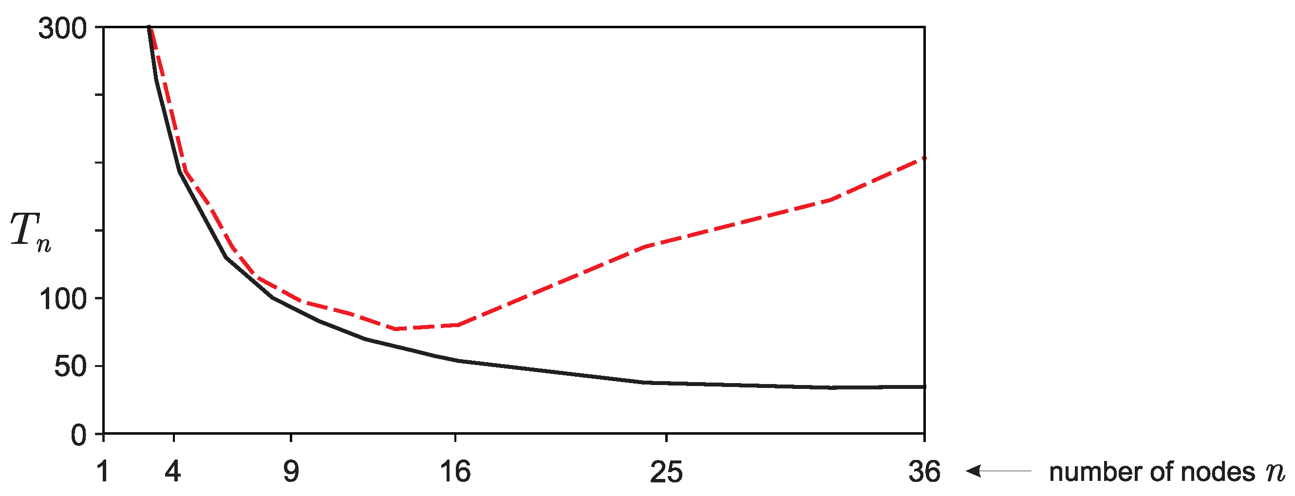
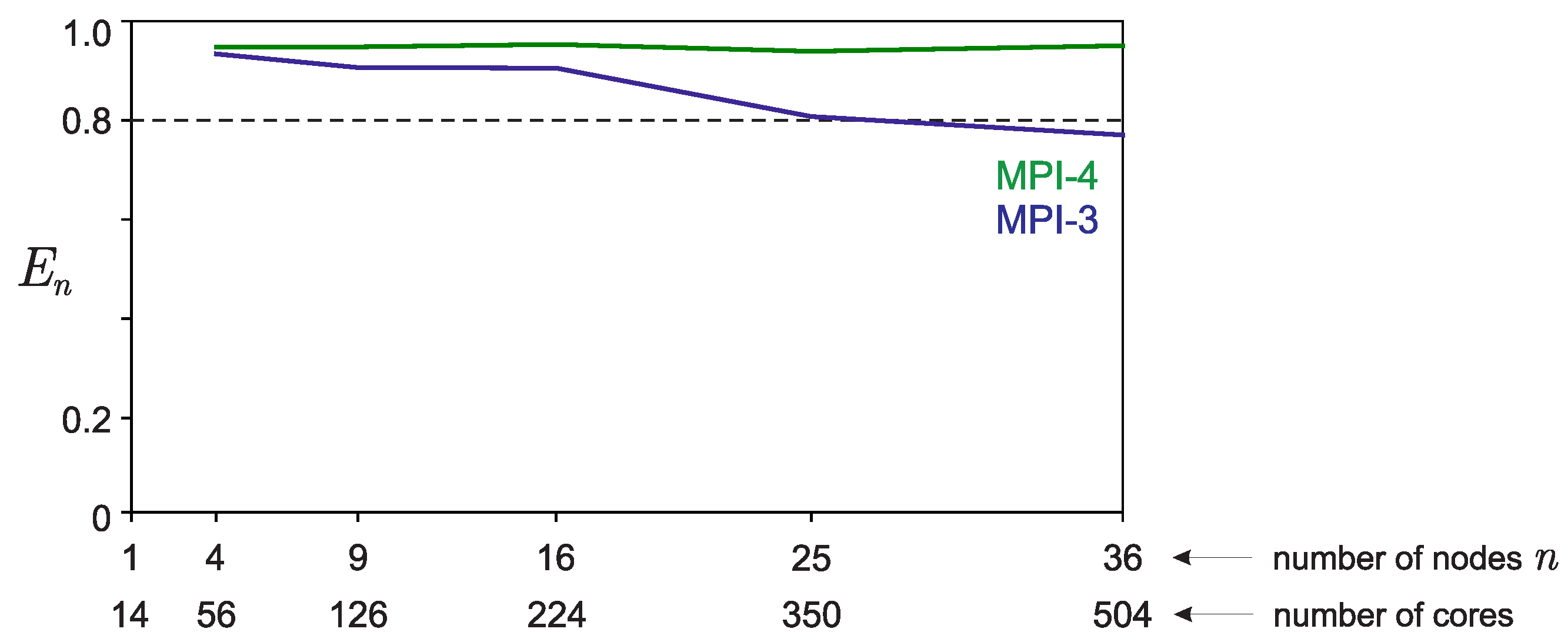
5.2. Scalability: Strong and Weak Scaling

It is well known that the weak point of parallel algorithms for solving systems of linear algebraic equations with a dense matrix is the relatively poor strong scalability of many possible software implementations (as can be seen from Figure 5).
This can be explained as follows on the example of a parallel algorithm for matrix-vector multiplication (see Figure 3), which is the main operation in the considered Algorithms 3 and 4.
All MPI processes participate in parallel computations, and, as a result, all computations are accelerated by n times ( n numprocs). At the same time, the volume of transmitted messages is proportional to 1 n , which means that it decreases with an increase in the number of processes involved in the calculations. However, with an increase in the number of processes participating in calculations, the number of message exchanges between the processes of auxiliary communicators increases, which is proportional to log 2 n .
It turns out that with an increase in the number n of processes involved in calculations, the computation time is proportional to 1 n , and the time to exchange messages between processes is proportional to log 2 n n .
Thus, starting from a certain number of processes (this number depends on the computational size of the problem and on the configuration of the multiprocessor system), the portion of overhead costs for the exchange of messages between processes will begin to increase. This, as a consequence, will inevitably lead to a decrease in the efficiency of software implementation with an increase in the number of processes involved in the calculations.
Therefore, additional calculations were carried out to test the proposed software implementations for weak scalability. Weak scalability means maintaining efficiency as the number of processes participating in computations increases while keeping the amount of computational work that each process performs constant.
Thus, the weak scalability test was performed by simultaneously increasing the problem size ( M : = n 3 M , N : = n 3 N , s : = n 3 s ) and the number n of processes involved in the computation. Figure 7 shows graphs of the parallelization efficiency E n = T 1 T n depending on the number of computing nodes n involved in the calculations. As can be seen from the presented graphs, the proposed software implementations of the algorithm have the property of weak scalability. This again shows the advantage of using the MPI-4 standard.

6. Discussion

1.
All program examples are built in such a way that they can be easily rewritten using the C/C++/Fortran programming languages. This is due to the fact that all MPI functions used in Python software implementations use a syntax equivalent to the syntax of the corresponding MPI functions in the C/C++/Fortran programming languages.
2.
If there are GPUs on the computing nodes, the programs can be easily modified by replacing the main calculations using the function dot() from the package numpy with calculations using a similar function from the package cupy, which will allow for the use of GPUs for calculations. Thus, it is easy to use MPI+OpenMP+CUDA hybrid parallel programming technologies. Due to the fact that changes in the software implementation will be quite simple, the program code is not shown here.
3.
The algorithm is primarily designed to solve systems of linear equations with a dense matrix. It has not been tested for solving systems of linear equations with a sparse matrix. Due to the technical features of working with sparse matrices, it is possible that the results regarding the efficiency of software implementation may differ significantly (both for better and for worse). More research is required on this issue.
4.
If System (1) is ill-conditioned, then regularizing algorithms are usually used to solve it [29]. One of the important stages in the application of regularizing algorithms is the stage of choosing the regularization parameter, which must be consistent with the error in specifying the input data and the measure of inconsistency of the system being solved. The considered algorithm makes it possible to accurately estimate the measure of incompatibility of the system being solved.

7. Conclusions

In this work, a fairly efficient parallel algorithm for solving large overdetermined systems of linear algebraic equations with a dense matrix was proposed. This algorithm is based on the use of a modification of the conjugate gradient method, which is able to take into account rounding errors accumulated during of calculations when making a decision to terminate the iterative process. This modification of the conjugate gradient method is constructed in such a way that it was possible to hide additional calculations in a parallel software implementation against the background of message forwarding of the main part of the algorithm. Thus, the proposed parallel software implementation of the considered algorithm, on the one hand, makes it possible to obtain an adequate approximate solution, and, on the other hand, does not increase the computational complexity. Moreover, the undeniable advantage of using the modern MPI-4 standard in the software implementation of algorithms of this type has been demonstrated.

Funding

Russian Science Foundation (project 23-41-00002).

Institutional Review Board Statement

Not applicable.

Informed Consent Statement

Not applicable.

Data Availability Statement

Not applicable.

Acknowledgments

This research was carried out using the equipment of the shared research facilities of HPC computing resources at Lomonosov Moscow State University.

Conflicts of Interest

The author declare no conflict of interest.

References

  1. Demmel, J.W.; Heath, M.T.; Van Der Vorst, H.A. Parallel numerical linear algebra. Acta Numer. 1993, 2, 111–197. [Google Scholar] [CrossRef] [Green Version]
  2. Hestenes, M.; Stiefel, E. Methods of conjugate gradients for solving linear systems. J. Res. Natl. Bur. Stand. 1952, 49, 409. [Google Scholar] [CrossRef]
  3. Greenbaum, A. Iterative Methods For Solving Linear Systems; SIAM: Philadelphia, PA, USA, 1997. [Google Scholar]
  4. Kabanikhin, S. Inverse and Ill-Posed Problems: Theory and Applications; Walter de Gruyter: Berlin, Germany, 2011. [Google Scholar]
  5. Woźniakowski, H. Roundoff-error analysis of a new class of conjugate-gradient algorithms. Linear Algebra Its Appl. 1980, 29, 507–529. [Google Scholar] [CrossRef] [Green Version]
  6. Kaasschieter, E.F. A practical termination criterion for the conjugate gradient method. BIT Numer. Math. 1988, 28, 308–322. [Google Scholar] [CrossRef]
  7. Strakoš, Z. On the real convergence rate of the conjugate gradient method. Linear Algebra Its Appl. 1991, 154, 535–549. [Google Scholar] [CrossRef] [Green Version]
  8. Arioli, M.; Duff, I.; Ruiz, D. Stopping Criteria for Iterative Solvers. SIAM J. Matrix Anal. Appl. 1992, 13, 138–144. [Google Scholar] [CrossRef]
  9. Notay, Y. On the convergence rate of the conjugate gradients in presence of rounding errors. Numer. Math. 1993, 65, 301–317. [Google Scholar] [CrossRef]
  10. Axelsson, O.; Kaporin, I. Error norm estimation and stopping criteria in preconditioned conjugate gradient iterations. Numer. Linear Algebra Appl. 2001, 8, 265–286. [Google Scholar] [CrossRef] [Green Version]
  11. Arioli, M.; Noulard, E.; Russo, A. Stopping criteria for iterative methods: Applications to PDE’s. Calcolo 2001, 38, 97–112. [Google Scholar] [CrossRef]
  12. Strakoš, Z.; Tichỳ, P. On error estimation in the conjugate gradient method and why it works in finite precision computations. Electron. Trans. Numer. Anal. 2002, 13, 56–80. [Google Scholar]
  13. Arioli, M. A stopping criterion for the conjugate gradient algorithm in a finite element method framework. Numer. Math. 2004, 97, 1–24. [Google Scholar] [CrossRef] [Green Version]
  14. Meurant, G. The Lanczos and Conjugate Gradient Algorithms: From Theory to Finite Precision Computations; SIAM: Philadelphia, PA, USA, 2006. [Google Scholar]
  15. Chang, X.W.; Paige, C.C.; Titley-Peloquin, D. Stopping Criteria for the Iterative Solution of Linear Least Squares Problems. SIAM J. Matrix Anal. Appl. 2009, 31, 831–852. [Google Scholar] [CrossRef] [Green Version]
  16. Jiránek, P.; Strakoš, Z.; Vohralík, M. A posteriori error estimates including algebraic error and stopping criteria for iterative solvers. SIAM J. Sci. Comput. 2010, 32, 1567–1590. [Google Scholar] [CrossRef] [Green Version]
  17. Landi, G.; Loli Piccolomini, E.; Tomba, I. A stopping criterion for iterative regularization methods. Appl. Numer. Math. 2016, 106, 53–68. [Google Scholar] [CrossRef]
  18. Rao, K.; Malan, P.; Perot, J.B. A stopping criterion for the iterative solution of partial differential equations. J. Comput. Phys. 2018, 352, 265–284. [Google Scholar] [CrossRef]
  19. Carson, E.C.; Rozložník, M.; Strakoš, Z.; Tichý, P.; Tůma, M. The Numerical Stability Analysis of Pipelined Conjugate Gradient Methods: Historical Context and Methodology. SIAM J. Sci. Comput. 2018, 40, A3549–A3580. [Google Scholar] [CrossRef]
  20. Cools, S.; Yetkin, E.F.; Agullo, E.; Giraud, L.; Vanroose, W. Analyzing the effect of local rounding error propagation on the maximal attainable accuracy of the pipelined conjugate gradient method. SIAM J. Matrix Anal. Appl. 2018, 39, 426–450. [Google Scholar] [CrossRef] [Green Version]
  21. Greenbaum, A.; Liu, H.; Chen, T. On the Convergence Rate of Variants of the Conjugate Gradient Algorithm in Finite Precision Arithmetic. SIAM J. Sci. Comput. 2021, 43, S496–S515. [Google Scholar] [CrossRef]
  22. Polyak, B.; Kuruzov, I.; Stonyakin, F. Stopping Rules for Gradient Methods for Non-Convex Problems with Additive Noise in Gradient. arXiv 2022, arXiv:2205.07544. [Google Scholar]
  23. Lukyanenko, D.; Shinkarev, V.; Yagola, A. Accounting for round-off errors when using gradient minimization methods. Algorithms 2022, 15, 324. [Google Scholar] [CrossRef]
  24. De Sturler, E.; van der Vorst, H.A. Reducing the effect of global communication in GMRES(m) and CG on parallel distributed memory computers. Appl. Numer. Math. 1995, 18, 441–459. [Google Scholar] [CrossRef]
  25. Eller, P.R.; Gropp, W. Scalable non-blocking preconditioned conjugate gradient methods. In Proceedings of the SC’16: Proceedings of the International Conference for High Performance Computing, Networking, Storage and Analysis, Salt Lake City, UT, USA, 13–18 November 2016; pp. 204–215. [Google Scholar] [CrossRef]
  26. DAzevedo, E.; Romine, C. Reducing Communication Costs in the Conjugate Gradient Algorithm on Distributed Memory Multiprocessors; Technical Report; Oak Ridge National Lab.: Oak Ridge, TN, USA, 1992. [Google Scholar]
  27. Dongarra, J.J.; Duff, I.S.; Sorensen, D.C.; Van der Vorst, H.A. Numerical Linear Algebra for High-Performance Computers; SIAM: Philadelphia, PA, USA, 1998. [Google Scholar]
  28. Voevodin, V.; Antonov, A.; Nikitenko, D.; Shvets, P.; Sobolev, S.; Sidorov, I.; Stefanov, K.; Voevodin, V.; Zhumatiy, S. Supercomputer Lomonosov-2: Large Scale, Deep Monitoring and Fine Analytics for the User Community. Supercomput. Front. Innov. 2019, 6, 4–11. [Google Scholar] [CrossRef] [Green Version]
  29. Tikhonov, A.; Goncharsky, A.; Stepanov, V.; Yagola, A. Numerical Methods for the Solution of Ill-Posed Problems; Kluwer Academic Publishers: Dordrecht, The Netherlands, 1995. [Google Scholar]
Figure 1. Graph of dependence of x n r e s component values on component number n.
Algorithms 16 00242 g001
Figure 2. An example of data distribution among nine MPI processes that form a 3 × 3 grid.
Algorithms 16 00242 g002
Figure 3. A parallel algorithm for matrix–vector multiplication in the case of a two-dimensional division of the matrix into blocks.
Algorithms 16 00242 g003
Figure 4. A parallel algorithm for multiplying a transposed matrix by a vector in the case of two-dimensional division of a matrix into blocks.
Algorithms 16 00242 g004
Figure 5. Plots of parallelization efficiency depending on the number of computing nodes for various software implementations of the parallel algorithm. Strong scalability is present only for software implementation using the standard MPI-4.
Algorithms 16 00242 g005
Figure 6. Graphs of the dependence of the parallel program running time in the case of good localization of computing nodes in the communication network (solid line) and poor localization (dotted line).
Algorithms 16 00242 g006
Figure 7. Graph showing the weak scalability of the proposed software implementations.
Algorithms 16 00242 g007
Disclaimer/Publisher’s Note: The statements, opinions and data contained in all publications are solely those of the individual author(s) and contributor(s) and not of MDPI and/or the editor(s). MDPI and/or the editor(s) disclaim responsibility for any injury to people or property resulting from any ideas, methods, instructions or products referred to in the content.

