Fully Parallel Homological Region Adjacency Graph via Frontier Recognition

Abstract

Relating image contours and regions and their attributes according to connectivity based on incidence or adjacency is a crucial task in numerous applications in the fields of image processing, computer vision and pattern recognition. In this paper, the crucial incidence topological information of 2-dimensional images is extracted in an efficient manner through the computation of a new structure called the HomDuRAG of an image; that is, the dual graph of the HomRAG (a topologically consistent extended version of the classical RAG). These representations are derived from the two traditional self-dual square grids (in which physical pixels play the role of 2-dimensional cells) and encapsulate the whole set of topological features and relations between the three types of objects embedded in a digital image: 2-dimensional (regions), 1-dimensional (contours) and 0-dimensional objects (crosses). Here, a first version of a fully parallel algorithm to compute this new representation is presented, whose timing complexity order (in the worst case and supposing one processing element per 0-cell) is $O\left(log\right(M\times N\left)\right)$ , M and N being the height and width of the image. Efficient implementations of this parallel algorithm would allow images to be processed in real time, as well as permit us to uncover fast algorithms for contour detection and segmentation, opening new perspectives within the image processing field.

1. Introduction

Having at hand a representation where an image’s content can be accessed in logarithmic time would allow the development of efficient image processing methods. Such methods might be able to deal with the ever-increasing sizes of the images that are currently used to solve pattern recognition problems, such as video and image segmentation (i.e., [1]), object detection (i.e., [2]), etc. To this respect, Region Adjacency Graph ($RAG$) representations for digital images are intuitive models that are useful for numerous applications in the field of region segmentation and pattern recognition by relating regions and their attributes according to their adjacencies. $RAGs$ represent the neighboring relationships of regions, resulting in simple graphs (no parallel edges, no self-loops). Algorithms based on a combination of graphs, color processing methods and enhanced with region growing or watershed transformation have been used for many decades in order to segment color images [3]. Unfortunately, these techniques present several limitations such as over-segmentation, high sensitivity to noise and poor detection of some boundaries [4]. However, the inherent labeling of two-dimensional structures (such as regions) in order to detect the complete set of region adjacencies implies a difficult processing, which conveys to algorithms that are mostly sequential, or, maybe, having a modest degree of parallelism if the labeling is started at the same time in several pixels (usually called ”seeds”). 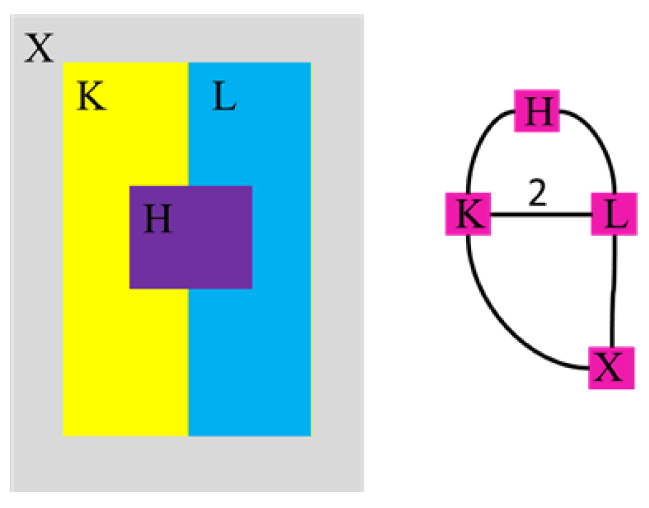The resultant $RAG$ must be expressed as a graph, whose nodes are image regions, each one having a variable number of edges (which represent region adjacencies). 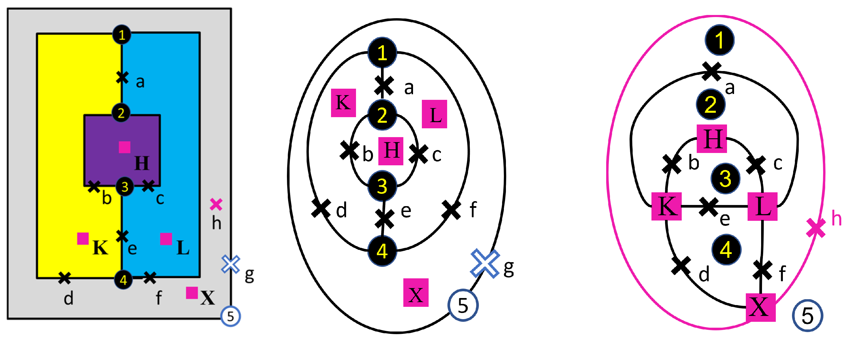For instance, a simple $RAG$ example is given in Figure 1 on the right for the image in Figure 1 on the left. Although this image contains only four regions, it does present two special topological relations among them that are not accurately represented by a simple graph: $\left(1\right)$ the presence of multiple contacts (between regions K and L in this image), which supposes multiple edges in the $RAG$, and $\left(2\right)$ the existence of holes in a region (as it happens in region X), which should be correctly addressed if topology properties are to be preserved within the $RAG$. The first issue can be avoided by using weights at the corresponding edges (the number 2 shown in Figure 1 on the right), but the second problem has not been formally considered in most of the current literature. There have been some interesting proposals in this direction, such as those of generalized maps [5], which are topological models that allow us to represent generic subdivided objects. These topological issues have also been addressed by using multigraphs (graphs containing parallel edges and/or self-loops [6]).

A topologically consistent representation [7] is the one that “shows the interactions between regions and then realize the topology of the image”. In this sense, $RAGs$ are not topologically consistent representations, even in 2D, since one can find topologically different images that would be represented by the same $RAG$ [8].

In order to keep computing simplicity and to promote parallelism while preserving the topological relations within the required multi-object structure, we propose embedding these objects into an abstract cell complex ($ACC$) [9] that is enriched with cell incidences. In this way, this image encoding allows us to compile an image’s statistics under a consistent topological format (see the

Table 1. Mean results of five executions for a set of random images with different number of colors and densities for B/W images. From left to right: size $M\times N$, number of colors, density, number of iterations of Stage 1, absolute number of representative homology cells of dimensions 0 and 1, normalized execution times of Stages 1 and 2, and normalized sum of the number of representative homology cells of dimension 0.

M = N	Number of Colors	Density	Number of Iterations Stage 1	n0,3	n0,4	n0,2	n1, mono	n1, reg,mono	n0,3 + n0,4 + n0,2	Normalized Time Stage 1	Normalized Time Stage 2	Normalized n0,3 + n0,4 + n0,2
50	2	0.1	7.0	29.2	34.6	124.4	124.4	124.4	188.2	6.7	1.2	1.6
50	2	0.3	5.6	88.0	212.6	58.0	58.0	58.0	358.6	2.2	2.6	3.0
50	2	0.5	6.2	97.2	299.6	12.8	12.8	12.8	409.6	2.2	3.3	3.4
50	2	0.7	5.6	80.8	201.0	65.4	65.4	65.4	347.2	2.3	2.5	2.9
50	2	0.9	6.4	33.2	42.8	115.8	115.8	115.8	191.8	7.7	1.3	1.6
50	3	1	4.4	832.8	530.4	0.4	0.4	0.4	1363.6	3.9	9.7	11.4
50	4	1	3.4	1046.4	799.2	0.0	0.0	0.0	1845.6	7.8	14.0	15.4
50	5	1	3.4	1082.4	998.2	0.2	0.2	0.2	2080.8	9.1	15.5	17.4
50	6	1	3.0	1055.6	1166.4	0.0	0.0	0.0	2222.0	17.4	18.6	18.6
50	7	1	2.8	1016.8	1289.0	0.0	0.0	0.0	2305.8	16.5	18.4	19.3
50	8	1	2.8	960.8	1395.2	0.0	0.0	0.0	2356.0	14.8	18.3	19.7
100	2	0.1	6.6	74.0	152.2	500.4	500.4	500.4	726.6	9.8	3.0	6.1
100	2	0.3	6.0	162.0	860.6	269.0	269.0	269.0	1291.6	8.6	9.4	10.8
100	2	0.5	6.6	206.0	1213.4	52.4	52.4	52.4	1471.8	8.1	12.5	12.3
100	2	0.7	6.0	168.0	848.0	262.4	262.4	262.4	1278.4	7.9	9.1	10.7
100	2	0.9	6.4	74.8	154.0	506.0	506.0	506.0	734.8	11.6	3.1	6.1
100	3	1	4.4	3115.6	2194.6	4.4	4.4	4.4	5314.6	7.4	38.3	44.4
100	4	1	4.0	3980.0	3173.8	0.0	0.0	0.0	7153.8	15.5	52.2	59.8
100	5	1	3.6	4072.0	4068.0	0.2	0.2	0.2	8140.2	20.8	66.0	68.1
100	6	1	3.0	3912.0	4790.8	0.0	0.0	0.0	8702.8	29.7	71.6	72.8
100	7	1	3.0	3776.4	5338.2	0.0	0.0	0.0	9114.6	74.6	81.1	76.2
100	8	1	2.8	3559.6	5791.2	0.0	0.0	0.0	9350.8	73.3	78.7	78.2

), which is crucial for current relevant computer vision problems such as contour detection, superpixel generation, image simulation or even artificial intelligence.

The $ACC$ framework can completely embed digital image components (with cells of different dimensions) and their incidences (bounding or cobounding relations) (see Section 3). Homological (adjacency) information of the image is understood here in the context of the square grid associated to the $ACC$ model of the image: (a) at 0 level, in terms of a maximally connected set of cells (connected components (CCs)) of the dimension i through cells of dimension $i-1$ or $i+1$; (b) at 1 level, in terms of the homological holes presenting in each $ACC$ version of the previous connected components (see [10]).

Going further, the proposed algorithm is completely written using matrices, which appear to be very efficient in modern computers.

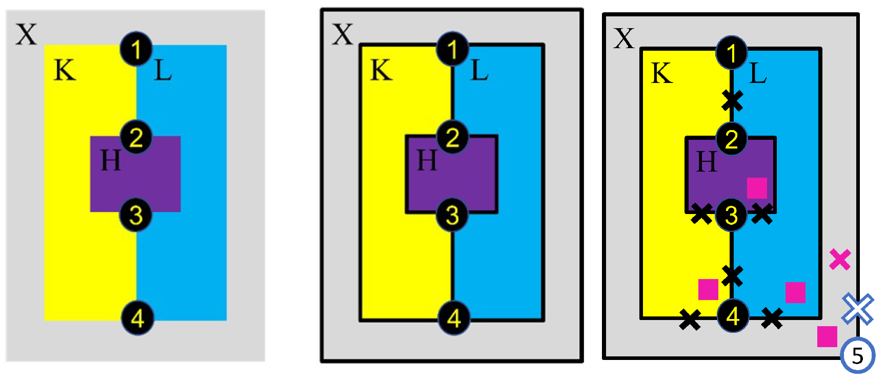
In order to clarify the previous concepts, Figure 2 depicts, in three steps, the complete homological information of Figure 1, which consists of the following: $\left(1\right)$ Figure 2, left, highlights crosses among regions, which correspond to zero-dimensional objects; $\left(2\right)$ in Figure 2, center, frontiers have been added as unidimensional objects; and $\left(3\right)$ Figure 2, right, draws the two-, one- and zero-dimensional homological representative elements of this image, given by squares, crosses and circles, respectively. Note that the region X has a hole, and a 1-dimensional element colored as a pink cross is added to differentiate it from the other 1-dimensional frontier’s representatives. Likewise, the most external frontier presents a hole; thus, a 0-dimensional representative (marked as 5) must appear.

It is worth highlighting that having correctly determined the complete homological information, the Euler number of the whole set of open separated objects is 1 (because no object intersection exists). In the case of Figure 2, the set of independent objects is composed of: four regions (one of them with a hole), seven frontiers (one of them having another hole), and four crosses. The  Euler number of the set of independent objects is 1, and it can also be calculated according to $n_2-n_1+n_0=1$, $n_k$ being the number of representative cells of dimension k (which can be CCs or holes): $4(2-d)-[7+1(pinkcross\left)\right](1-d)+[4+1(whitecircle\left)\right](0-d)$.

For the rest of the paper, we consider a digital image I with $M\times N$ pixels having 4-adjacencies among them. We have designed and implemented a parallel algorithm for computing the homological relations among the frontiers and crosses of the given image. The parallel algorithm described here allows us to foresee that the theoretical time complexity of the whole process is to be the logarithm of the width plus height of the image when enough processing elements are available.

The rest of the paper has been organized in the following sections. After reviewing the previous studies in this field (Section 2), we briefly define the $ACC$ framework (Section 3) that allows us to correctly express both the HomRAG and HomDuRAG, whose relations are discussed in Section 4. Section 5 describes the proposed parallel algorithm, and Section 6 contains a detailed example of its procedure which is a mechanism to check its correctness and remarkable preliminary results. Finally, the conclusions and foreseeable future extensions are debated in the last section, Section 7.

2. Related Work

There are numerous works that represent images as neighborhood graphs. For example, nodes can represent pixels of the image, and edges the connection between adjacent pixels. If the 4-adjacency relation for pixels is considered, the topological information can be condensed into a graph, where regions will be represented by nodes, and edges are boundaries between regions. $RAG$ representations are useful and intuitive models to be used for image segmentation problems, but, usually, difficult and complicated algorithms are required to manage $RAG$ native graph structures. In this sense, working with edges or contours can produce enhanced image segmentations but with an efficiency that must be carefully analyzed because graph approaches are commonly impractical for large graphs [11].

On the other hand, although connected-component analysis (CCA) has been used in the last decade in many imaging applications (X-ray computed tomography, medical imaging, real-time automotive applications, etc.), and parallel algorithms for them are appearing [12], our proposal here tries to go further by considering the complete set of adjacency relations among CCs.

More complex representations have been developed to overcome the aforementioned $RAG$ problems. For example, in dual graphs [13], images are represented by a pair of finite planar graphs that are dual to each other. These graphs allow the construction of a hierarchy of partitions (dual graph pyramids). Furthermore, processing these two graphs may not provide an efficient result; therefore, its application to real images has been quite limited.

In [14], it was proved that a topologically consistent representation of an n-dimensional segmentation requires explicit representation of all cell types up to dimension n. Combinatorial maps [15] are representations of an image as a set of half-edges, called darts, and two permutation functions. They store cells and their adjacencies and encode the topology of their embedding into 2D space. These maps have certain limitations: (a) they require a massive number of auxiliary darts, so they are not feasible for big images, and (b) they are difficult to manipulate. In this paper, we used the ACC representation [10], which needs significantly less storage and allows a “smooth” transference to adjacency graph representations [16]. It compiles numerous local and global topological statistics of the image at a cellular level that allow it to be analyzed from a probabilistic or fractal point of view [17].

Hence, the efficient construction of $RAG$ is a rare topic in the literature, and it has usually been related to methods for computing max and min trees and other hierarchical representations.

There is plenty in the literature dealing with homological tools applied to digital images (see, for instance, [18,19,20]). In this paper, we follow the principles and ideas provided by the Homological Spanning Forest ($HSF$) model of the image [21]. Using this parallel combinatorial technique, the processing of high-level segmentations can be solved through topological reductions in $ACCs$ and leads to improved parallel processing to every n-dim cell and incidence of the image where computing time was near the logarithm of the width plus the height of the image. In this sense, another type of representation is the so-called $CRIT$ (Contour Region Incidence Tree, [17]); that is, a topologically informative connectivity graph, extracted by compacting an image’s $ACC$ and whose 2-cells represent the image’s constant color regions. The $CRIT$ overcomes the previous difficulties of the $RAG$ and is a topologically consistent representation, which is obtained using the previously mentioned Homological Spanning Forest ($HSF$). Other parallel algorithms for computing $RAG$ information through the Homogeneous Spanning Forest model under an $ACC$ scenario have been developed in [19,22].

In conclusion, cell complex representation is an ideal mathematical scenario for extracting topological image properties that straightforwardly promote from local to global magnitudes, with the additional advantage that these global properties will be robust under deformations, translations and rotations. Currently, these properties are extracted using topological invariants such as homology or Euler’s number. Let us note that Betti numbers and Euler’s number are the only topological invariants that have been managed using parallel approaches [23,24]. Therefore, the approach proposed here will simplify the $HSF$ framework in order to manage only one of the two trees that can be defined in planar images. However, we show here that this single tree will be enough to completely represent incidence relations for all embedded objects in the image and to deduce other information such as the number of regions.

3. A Simplified ACC Framework

The proposed topological framework for digital images is based on a simplification of the classical abstract cell complex concept ($ACC$) [9]. In a few words, an $ACC$ consists of a set of cells of different dimensions which are endowed with a transitive bounding relation between cells of contiguous dimensions, thus having no bounding relation for pairs of cells with dimensions differing by more than one. Therefore, given a 2D digital image I, the proposed $ACC$ consists of physical pixels (represented by 2-cells), frontiers between pixels (that is, interpixel elements represented by 1-cells) and adjacencies between frontiers (or corners between pixels, represented by 0-cells) (an example is depicted in Figure 3). The bounding relations among different cells can be easily inferred for this kind of square $ACC$ according to this figure. We refer the reader to [9] for a more strict definition. It is assumed that an external region surrounds the whole image, having different attributes (for example, color) than any of the image’s pixels. Hence, the image borders are extended with additional 0- and 1-cells so that the whole $ACC$ is a compact set, which ensures that its Euler number is always 1.

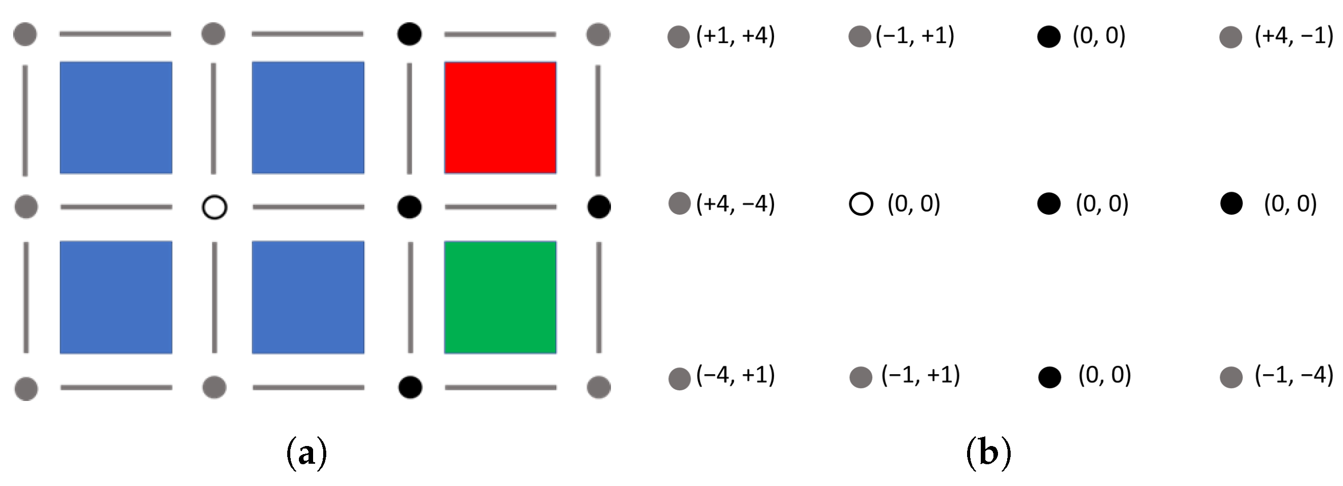
In order to compute HomDuRAG, 0-cells are firstly classified into three main types: crosses, frontiers between regions, and points inside an object. In Figure 3, they are represented by black, gray and empty circles, respectively. This first classification is performed by comparing the attributes of the set of four pixels surrounding each 0-cell. Crosses appear when three or four pixels with different attributes (colors, for example) surround the 0-cell; frontiers appear when there are two different sets of contiguous identical pixels, and interior 0-cells appear if the four pixels are identical. For example, in Figure 3, a single interior 0-cell is inside the blue region. Up to four crosses appear between red, blue, green and external regions. Finally, the rest of 0-cells are frontiers between two regions. Distances between any pair of 0-cells must be calculated so that the algorithm detailed in Section 5 can determine the two extremes of each frontier. In Figure 3, on the right, pairs of distances are shown for each 0-cell; note that crosses and interior 0-cells have zero values, while the other cells point towards two directions, being −4 for North, +4 for South (because 4 is the number of columns $Nc=N+1$), −1 for West and +1 for East in this example (matrices are supposed to be stored in row-major order, as usual).

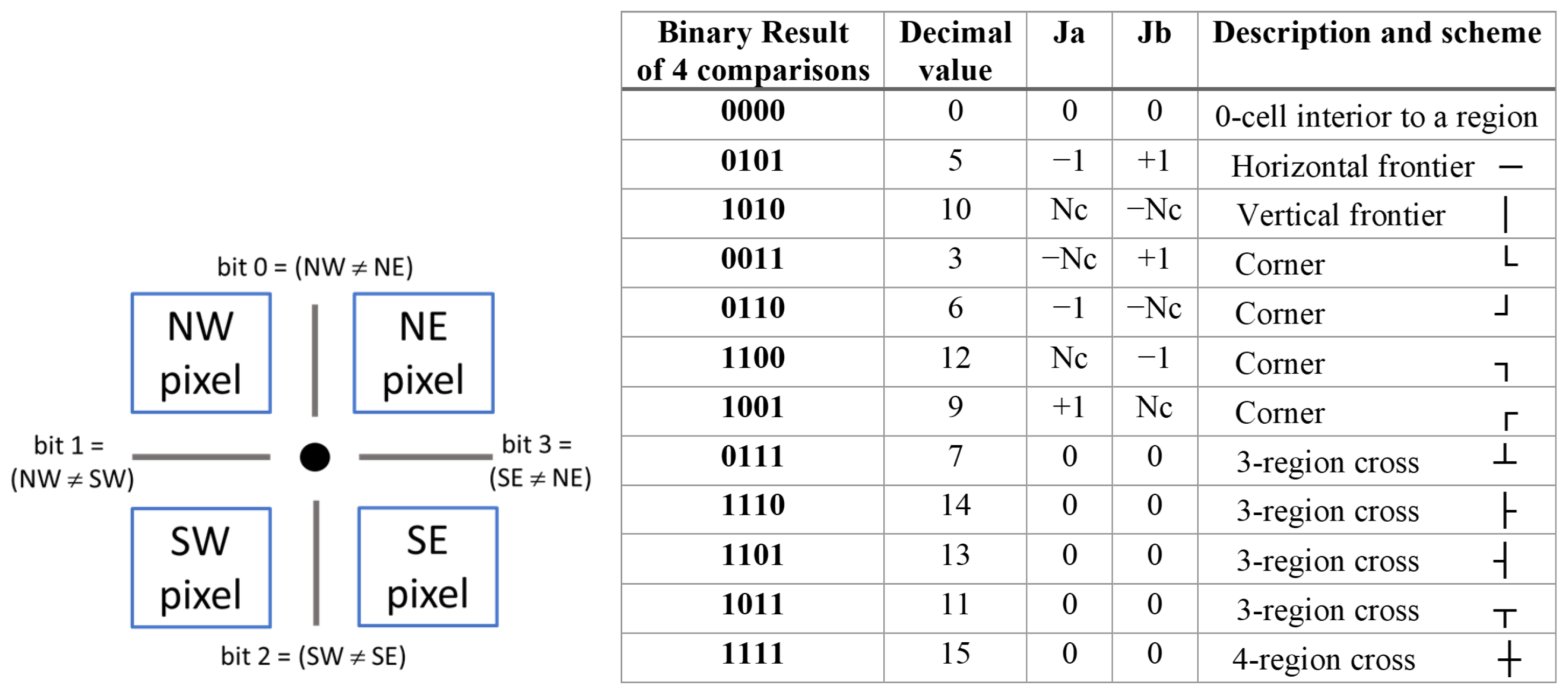
To be precise, the comparison of pairs of adjacent pixels (which correspond to $ACC$ 1-cells) around a 0-cell yields to 4 binary values (Figure 4, left). Each of these comparisons results in a true/false bit, thus giving a total of 16 cases. Figure 4, right, shows the 12 possible cases because a set of comparisons where three are true (1) and one is false (0) is evidently impossible by the transitive property of equality. Classifying each 0-cell according to this table, it is easy to compute its pair of jump distances (called $Ja$ and $Jb$ here). Once the initial jump distances for all 0-cells are set, only these 0-cells will be used to compute HomDuRAG, meaning a matrix with (M + 1) × (N + 1) elements. Using this matrix, HomDuRAG can be efficiently extracted as explained in the next sections, and its relation with HomRAG can be foreseen by considering duality with the HomDuRAG.

4. Specifying Bijective HomRAG and HomDuRAG

Figure 2 depicted the complete homological information of a given image. Although this is a particular and small example, it contains all possible kinds of homological representatives for a subdivided digital image. Therefore, the relations among them can be straightforwardly obtained. The description and one example of each incidence relation in Figure 5, center, includes: (a) An incidence between a cross and a frontier; that is, between a 0- and 1-cell, such as edges ‘1a’, ‘2c’, ‘3e’, etc. (b) An incidence between a frontier hole and the frontier that contains it; that is, between a 0- and 1-cell, such as the double-edge ‘5g’. The description and one example of each incidence relation in Figure 5, right, includes: (c) An incidence between a frontier and a region; that is, between a 1- and 2-cell, such as edges ‘bH’, ‘cL’, ‘fX’, etc. (d) An incidence between a region hole and the region that contains it; that is, between a 1- and 2-cell, such as the double-edge ‘hX’.

Hence, depending on the required application, two adjacency graphs can be calculated and managed:

(1)

The graph with the homological information for crosses and frontier holes, which can be called HomDuRAG (Figure 5, center).

(2)

The graph with the homological information for regions (including adjacencies for region holes); that is, the HomRAG (Figure 5, right).

Obviously, these two graphs are planar as they come from a planar digital image. The duality among them can be established if the previously discussed particularities of the multiple and self-loop edges were taken into account. In this respect, faces (which are nodes in the dual graph) of the HomDuRAG have been drawn in the center of Figure 5 (Figure 5, right, respectively). Note the special case of the frontier hole numbered as 5, which is the face among the frontier h and the hypothetical external region outside the image (not drawn here). The task of computing an application for the mutual conversions of these graphs is not developed here due to lack of space, and it is intended for future work.

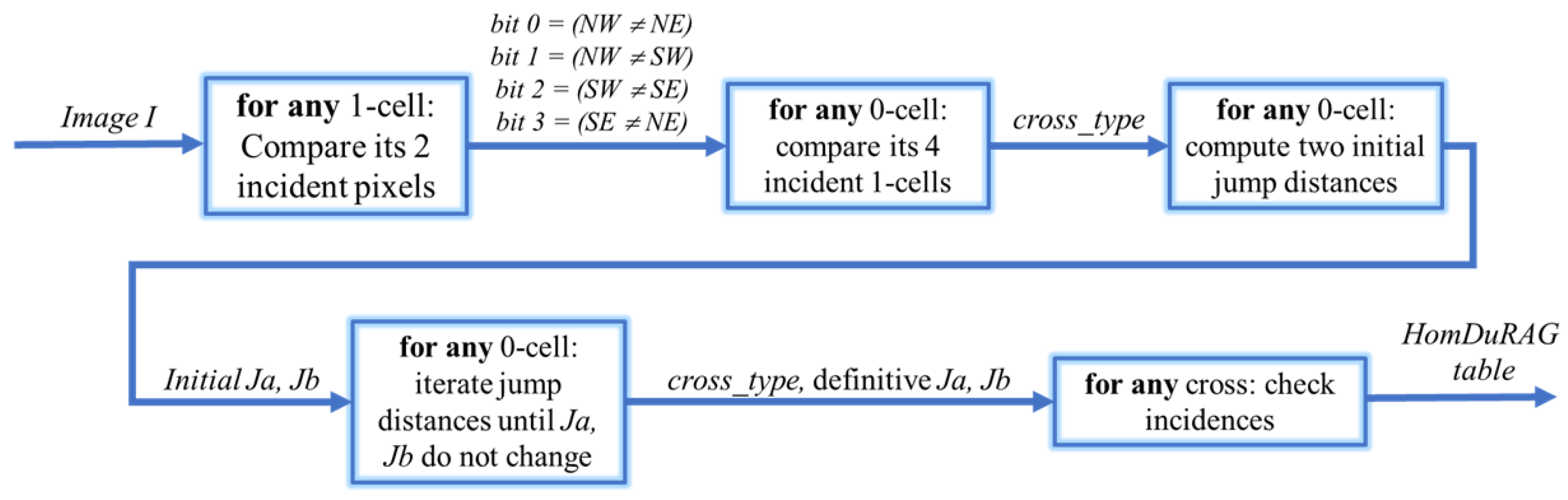
5. Parallel Algorithm for Computing the HomDuRAG

The entire process is schematically shown in the block diagram in Figure 6. The first two steps have been detailed in Section 3, where the associated $ACC$ is initialized, for the later computation of jump distances between 0-cells.

Having computed 0-cell types according to Figure 4, as well as  the jump distances to each adjacent 0-cell (Steps 1, 2, 3 of Algorithm 1), distances from every cell to the two crosses where its frontier ends can be computed in a fully parallel manner. The core of the algorithm is represented in Figure 7, and the regular situation proceeds as follows. At each iteration (Steps 4 and 5 of Algorithm 1), any cell keeps the jump distances towards the two directions of the frontier, called $Ja$ and $Jb$. Each 0-cell asks the cells pointed out by these jumps $Ja$ and $Jb$ which distances they hold ($J{a}_{neigh}$ at Step 4.b of Algorithm 1 and $J{b}_{neigh}$ at Step 4.d). If the distance $J{a}_{neigh}$ does not fall into a cross (which always maintains zero values for jump distances), the current 0-cell adds these neighbor values in two separate variables (Figure 7, left): $J{a}_{next}$ = $J{a}_{neigh}$ + $Ja\left(c\right)$, and $J{a}_{next-other}$ = $Jb(c+Ja(c\left)\right)+Ja\left(c\right)$ (Step 4.c of Algorithm 1). Then, the cell must choose the non-null between $J{a}_{next}$ and $J{a}_{next-other}$. Thus, $J{a}_{next}$ or $J{a}_{next-other}$ are stored in the 0-cell (Steps 4.c.ii or 4.c.iii of Algorithm 1). This would continue until the cell reaches a cross; thus, no further computation is needed (Figure 7, center). This last condition supposes a stop condition in the loop iteration for this 0-cell. It is worth noting the necessary condition to ensure that the jump distances are continuously increasing towards the correct direction (Steps 4.c.ii or 4.c.iii of Algorithm 1). Because it is impossible to know which direction each $Ja$ and $Jb$ are holding, the results for $J{a}_{next}$ and $J{a}_{next-other}$ may yield to a null value if the taken $J{a}_{neigh}$ (or $J{b}_{neigh}$ ) goes towards the opposite direction to the initial $Ja$ (or $Jb$). In this case, the sum $J{a}_{next}$ (or $J{a}_{next-other}$) would be null, and the opposite value, $J{a}_{next-other}$ (or $J{a}_{next}$), is the one that must be stored in the 0-cell. For the other direction, a similar procedure must be performed (Step 4.d of Algorithm 1). As is usual in synchronous cellular automaton algorithms, two pairs of matrices must always be kept: the current ones ($Ja$, $Jb$) and the newest values ($J{a}_{new}$, $J{b}_{new}$). So, any cell can compute its next jumps as a function of the previous state. Correspondingly, before proceeding with the next loop iteration (Step 4.e of Algorithm 1), the roles of these two pairs are interchanged.

A special case is needed to detect cycles in frontiers, such as that of the external frontier of region X in Figure 2. In cycles, the increasing operations of the previous loop would never stop because cycles present no crosses. Labeled 0-cells can be used to detect if jump distances are cycling around; when a 0-cell label (L1a in Figure 7, right) matches that of one of its pointed 0-cells (for example, L2 in the same figure), this means that the increasing operations have completely rounded a frontier, and, consequently, the procedure must stop. Labels can be propagated in a similar manner to jumps (for space reasons, the labeling process has not been specified in Algorithm 1; see the whole implementation in [25] for details). In our implementation, the most southeast corner is declared as the representative cell of the hole because it has the biggest label according to the initial one.

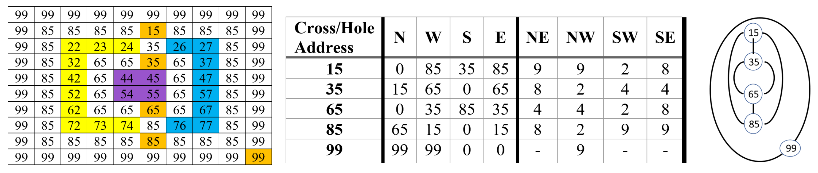
After a logarithmic number of iterations (because jump distances increase exponentially), any 0-cell has computed its distances to its two crosses, and the HomDuRAG can be extracted in a straightforwardd manner (Steps 6.a, 6.b and 6.c of Algorithm 1). Depending on the type of cross or hole frontier, these 0-cells must read the labels on their corresponding adjacent neighbors (given by the schemes in the last column of Figure 4) in order to fill table T. This set of neighboring labels condensed in table T is a minimal but complete representation of the HomDuRAG; each node (cross or hole frontier) knows its 2-, 3- or 4-adjacent nodes, thus having two, three or four edges.

Note that the “do…while” loop of the algorithm has been written in an identical and independent way for any 0-cell, and no carry ahead dependencies among iterations exist, thus facilitating its parallelization by simply dividing the matrices into disjoint sets of pieces. Only the variable $nHomc$ that counts crosses and holes in Steps 7.a, 7.b and 7.c would imply the need of a different counter for each processing element (such as CPU or GPU cores).

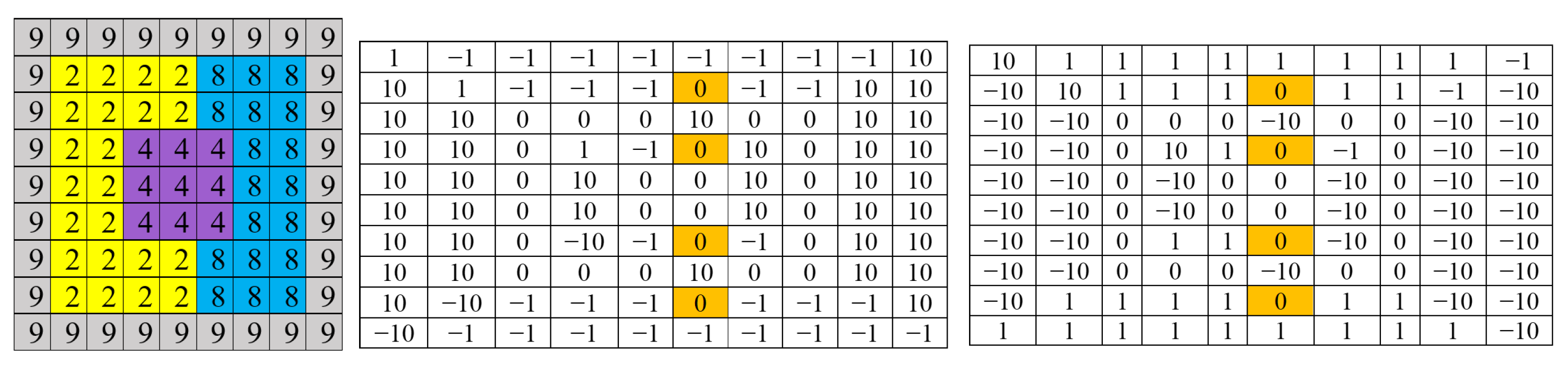
In order to clarify the proposed algorithm, a set of figures are depicted for a $M\times N=9\times 9$ image (Figure 8, left) that contains the same regions as those in Figure 1.

First of all, for any 0-cell c, jump distances $Ja\left(c\right)$, $Jb\left(c\right)$ are computed and stored in two $Nc\times Nc=10\times 10$ matrices (see Figure 8, center and right). Supposing that matrices are stored by rows, a value $Nc=10$ of distance means going South (respectively, −10, North). Interior 0-cells and crosses (among three regions depicted in orange for this image) are given a null jump.

Algorithm 1: Algorithm to compute jump distances for each 1-cell, building the jump distance matrix necessary to get the HomDuRAG

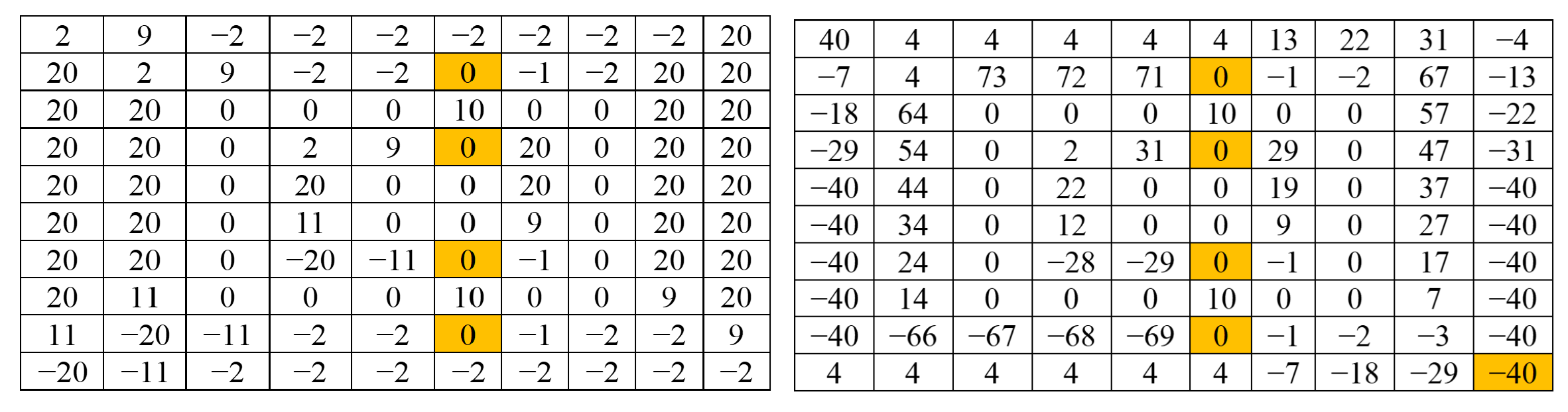
Later on, the main loop (Steps 4 and 5 of Algorithm 1) iterates. Figure 9 depicts values for $Ja$ at the end of two iterations: the first and last iterations (Iteration 5). During each iteration, jump distances are exponentially increased if no cross is reached. In our example and at the end of the first iteration, most 0-cells have doubled in distance (obvious for values, −2, 2, −20, and 20 and for −9, 9, −11, and 11 which mean that a row and column hop has been chosen). Only $Ja$ (or $Jb$, not shown here) remains with the same values (−1, 1, −10 or 10) when it has already reached a cross.

At the end of the loop, the $Ja$ value for each 0-cell points towards the corresponding cross. Note that jumps to the other direction are stored in $Jb$ (not shown here). The special case of a frontier cycle is solved as follows: the 0-cells that form the cycle have been exponentially increasing their $Ja$; thus, they have cycled around the perimeter with uninteresting values. However, thanks to the propagation of the biggest labels (99 for the case of the cycle, see Figure 10), the loop finishes at Iteration 5 when each cell detects that its own label matches that of its pointed 0-cell. At last, note that any 0-cell that is not interior to a region has been set to one of the cross labels (15, 35, 65 or 85) or to the representative label 99 of the cycle (see Figure 10). On the other hand, colored cells correspond to 0-cells inside regions (thus, labeling has not been performed for them).

Implementation of the presented method is quite straightforward when following the diagram of the algorithm in Algorithm 1. Although an optimized code for the current proposal has not yet been written, the following theoretical estimation of the time complexity is $O\left(log\right(M\times N\left)\right)$ if massive parallelism were employed, M and N being the width and height of image I, respectively. This is because the parallel algorithm for computing HomDuRAG follows the same logarithmic procedure for pixel jump calculation as in previous works such as for the Connected Compmonent Label Tree ($CCLT$) algorithm [21]—exponentially increasing jump distances through the iterations until no new jumps are assigned. Hence, it is expected that computation time costs reach those which occurred in the case of the $CCLT$.

6. Results

A complete implementation of the algorithm that computes the HomDuRAG has been performed in MATLAB/OCTAVE that serves to check the results for different types of images. The main script (scriptdualRAGimages.m) can load one of these sets of images at each time: (1) a synthetic image written in a matrix; (2) several random synthetic square images having a different number of colors and densities; (3) several synthetic square images containing an object with the longest perimeter; and (4) a real image.

After having loaded and checked an image, this main script launches dualRAGmainstages.m, which computes and checks the HomDuRAG by executing these stages in order:

(1) Script to compute jump distances for the 0-cells (dualRAG0celldetermination.m).

(2) Script to extract HomDuRAG expressed as a table T ($T\_crosses$ in the code) called dualRAGcountingcritcellsv1.m.

After computing HomDuRAG, a mechanism to check the correctness of those results concentrated in T has been written. First, frontiers are fused (script fusingfrontierCCs.m) as they were connected components (CCs). This fusion process returns the number of frontier CCs that contain more than one region ($n_{1,poly}$). With this number, homological representative cells of the regions embedded in the image can be completely derived using the Euler formula and the following calculation. The Euler number of the whole set of open separated objects is 1 (because no object intersection exists). In addition, the sum of all the Euler numbers can be calculated through the representative cells and can be expressed as $n_2-n_1+n_0=1$, $n_k$ being the number of representative cells of dimension k (which can be CCs or holes).

Clearly, $n_0$ can be computed via the table T; it is the total number of crosses with three or four pixels with different attributes (here described as $n_{0,3}$ and $n_{0,4}$, respectively) plus the number of holes composed of only one frontier (called $n_{0,2}$ in this work because the southeast-most 0-cell representative of any of these holes has only two cobounds).

With respect to $n_1$, it can be composed of four types of homological representative cells:

(a) Those corresponding to holes composed of only one frontier (that is, $n_{1,mono}$, which is equal to $n_{0,2}$).

(b) Those that must appear in regions that are outside each of these previous mono-frontier holes; $n_{1,reg,mono}$. Note that if the image border is a cycle, it cannot be counted in $n_1$ because this homological representative cell of dimension 1 would reside outside the whole image; thus, $n_{1,reg,mono}=n_{1,mono}-1$. On the contrary, $n_{1,reg,mono}$ = $n_{1,mono}$.

(c) Those that must emerge in regions that are outside each frontier CC containing more than one region. Again, if the image border belongs to one of these frontier CCs, the corresponding homological representative cell of dimension 1 would reside outside the whole image; thus, $n_{1,reg,poly}=n_{1,poly}-1$, being $n_{1,poly}$, the value calculated by the script fusingfrontierCCs.m. On the contrary, $n_{1,reg,poly}$ = $n_{1,poly}$.

(d) Each frontier itself not being a cycle represents a homological representative cell of dimension 1, which can be computed as half of the number of frontiers that go out of the crosses; that is, $(3\times n_{0,3}+4\times n_{0,4})/2$. Dividing by two is necessary because the cobounds of crosses are repeated twice, or, correspondingly, each frontier has two bounds.

In order to clarify this notation, let us resume Figure 2. This image contains four crosses with three pixels with different attributes ($n_{0,3}=4$) and one mono-frontier hole situated at the image border, labeled as 5 in the figure (that is, $n_{0,2}=1$). It contains no cross with 4 different pixels ($n_{0,4}=0$). By merging the frontiers, we obtain two frontier $CCs$: the external one that contains only region X, and the internal one that contains several regions. Then, $n_{1,mono}=1$ (but $n_{1,reg,mono}=0$ because this hole is on the image border), and $n_{1,poly}=1$ (further, $n_{1,reg,poly}=1$). In addition, the number of frontiers going out of crosses is $(3\times 4+4\times 0)/2=6$. The Euler formula yields the number of regions as:

$$\begin{array}{cc}{n}_2=\hfill & 1-n_0+n_1=\hfill \\ \hfill & 1-(n_{0,3}+n_{0,4}+n_{0,2})+\hfill \\ \hfill & n_{1,mono}+n_{1,reg,mono}+n_{1,reg,poly}+\frac{3\times n_{0,3}+4\times n_{0,4}}{2}=\hfill \\ \hfill & 1-(n_{0,3}+n_{0,4})+\hfill \\ \hfill & n_{1,reg,mono}+n_{1,reg,poly}+\frac{3\times n_{0,3}}{2}+2\times n_{0,4}\hfill \end{array}$$

(1)

For the case of Figure 2, $n_2=1-(4+0+1)+(1+0+1+6)=1-5+8=4$ regions (that is, regions X, K, H and L).

Once the number of regions has been computed with the previous formula, it is compared with that given by the sum of the number of regions returned by the MATLAB/OCTAVE method $bwlabel\left(\right)$ for each color. This comparison is checked in the script checkingresultsnofregions.m, ensuring the correctness of this implementation. Note that the last two scripts that serve to check results have been commented on in the uploaded implementation to prevent delays when computing HomDuRAG.

After testing several toy images similar to those in the previous figures (using Case 1 of  scriptdualRAGimages.m), the theoretical timing order was tested with images containing the largest perimeter (Case 2 of  scriptdualRAGimages.m); a zigzag object embedded in a background of a different color (see a $13\times 13$ zigzag image in Figure 11). The number of iterations of the algorithm to compute jump distances for the 0-cells that represent crosses and cycles ($n_{iter}$) matches the logarithm in base 2 of the semiperimeter of the zigzag (plus one iteration needed to escape from the main $while$ loop) as Figure 11 summarizes. This occurs because both jumps $J_a$ and $J_b$ (corresponding labels) grow exponentially from the southeast-most corner of the zigzag until they meet in the northwest-most corner. When both jumps meet, one additional iteration is required to demonstrate that any frontier has been completely labeled.

A third test that clearly reveals the timing order of the proposed algorithm is Case 3 of  scriptdualRAGimages.m—a set of random images with a different number of colors and densities (percentage of white pixels) for B/W images. The table in Table 1 shows the results obtained after five executions of images of sizes $50\times 50$ and $100\times 100$. The absolute numbers of representative homology cells $n_{0,\ast }$, $n_{1,\ast }$ are shown in this table. Moreover, in the last three columns, execution times and the sum of representative homology cells of dimension 0 have been normalized to that of a B/W $25\times 25$ image with a density of 0.5.

As expected, the number of crosses $n_{0,3}+n_{0,4}$ strongly depends on the number of colors. Note that even for an eight-color image, $n_{0,3}+n_{0,4}$ is very close to the number of 0-cells $(M+1)\times (N+1)$. In contrast, the number of frontier holes $n_{0,2}$ is greater for extreme densities (reaching a maximum for 0.1 and 0.9) and almost nonexistent for color images. In accordance with this, the required number of iterations to compute jumps and labels is inversely proportional to the number of colors because objects with a longer perimeter can appear for binary images, while colored image regions are usually composed of very few pixels.

Because of this, execution times of the second stage (script RAGcountingcritcellsv1.m) are mostly proportional to the sum $n_{0,3}+n_{0,4}+n_{0,2}$ because an entry in table T must be saved for each of these cells (see the last two columns of the table in Table 1). Execution times of the first stage (script dualRAG0celldetermination.m) are larger for images with a larger $n_{0,2}$ because they depend on the number of iterations to compute jumps and labels but also on the number of crosses $n_{0,3}+n_{0,4}$.

Finally, several tests were performed with real images, providing results similar to those of random images with many colors. This is not surprising since real images usually contain hundreds of colors, and the proposed algorithm goes through all 0-cells identically and independently of the pixel attributes.

It must be remembered that these timing results were obtained using MATLAB/Octave codes and with no parallel execution; future works must study the efficiency of our algorithms for modern parallel processors in which the number of threads/processes launched will considerably reduce these times and play an important role, aiming to reduce the dependence of timing on the image size and number of crosses.

7. Conclusions, Applications and Future Research

The presented method extracts the HomDuRAG of an image, which is the dual graph of the HomRAG (a topologically consistent extended version of the classical $RAG$). These representations encapsulate the whole set of topological features and relations between the three types of objects embedded in a digital image: 2-dimensional (regions), 1-dimensional (contours) and 0-dimensional objects (crosses). In this work, we have implemented a parallel version of an algorithm to compute HomDuRAG whose theoretical time complexity is $O\left(log\right(M\times N\left)\right)$, M and N being the image dimensions, via the set of $(M+1)\times (N+1)$ 0-cells of the $ACC$ that represents the image.

As such, the following tasks include the parallel implementation of the presented algorithm on a real-time framework and application. Both multicore CPUs and GPUs would probably fit for such objectives. Since the algorithm is fully parallel, HomDuRAG extraction promises to be computationally efficient so that it could be applied in numerous image processing subfields, such as image segmentation, matching, detection, reconstruction, etc.

Not only does HomDuRAG return directly topological features (set of holes, adjacencies, cell incidences, etc.), but it also can be modified to calculate other geometrical measures such as contour perimeters, contour curvatures, etc., because contours are completely labeled when building HomDuRAG. Hence, a complete set of an image’s statistics under a consistent topological format can be easily computed with our method, even extending this to a whole, specific dataset. As an objective of interest, this capability can be efficiently employed for pattern recognition using machine learning or optimization models among others. More specifically, giving an example on metaheuristic models, such as Genetic Algorithms, the extracted topological information of an image can be modeled as inputs of the fitness function or as genes presented in an individual in order to fine-tune a target image filter. Moreover, the extraction of features using our method can be a helpful support in deep learning since topological patterns are very difficult to learn, even through a large sequence of non-linear layers. Going further, we believe that the conversion of (big) data coming from different fields (such as medicine, transportation, robotics or computer networks among others) into synthetic images in order to calculate the previously mentioned set of topological statistics may open new possibilities regarding the modeling of advanced optimization algorithms and challenging decision problems, such as adaptive algorithms, island algorithms, hybrid heuristics and metaheuristics, polyploid algorithms, etc. This would improve the research performed by relevant references in these fields, including but not limited to the following: [26,27,28].

Another pending work is the implementation of an efficient and parallel algorithm for calculating HomRAG using HomDuRAG table T, having been shown here as a basic conversion that is possible thanks to the duality between both graphs.

Finally, a new field of image processing operations based on the table T is foreseeable because this table completely represents HomDuRAG and has two important advantages: it can be enlarged easily with the above-mentioned image information, and it is strictly ordered by the linear addresses of 0-cell labels.