Multiset-Trie Data Structure

Abstract

This paper proposes a new data structure, multiset-trie, that is designed for storing and efficiently processing a set of multisets. Moreover, multiset-trie can operate on a set of sets without efficiency loss. The multiset-trie structure is a search tree with properties similar to those of a trie. It implements all standard search tree operations together with the multiset containment operations for searching sub-multisets and super-multisets. Suppose that we have a set of multisets S and a multiset X. The multiset containment operations retrieve multisets from S that are either sub-multisets or super-multisets of X. We present the mathematical analysis of a multiset-trie that gives the time complexity of the algorithms and the space complexity of the data structure. Further, the empirical analysis of the data structure is implemented in a series of experiments. The experiments illuminate the time complexity space of the multiset containment operations.

1. Introduction

A multiset is a collection of elements that can have more than one instance. As in the case of ordinary sets, the ordering of the elements in multisets is not relevant. For example, multisets $\{1,1,2\}$ and $\{1,2,1\}$ represent the same multiset.

Multisets appear in a wide variety of domains and applications [1]. The index structures for storing sets of multisets were studied in the area of object-relational database systems to store, compress and query multiset-valued attributes efficiently [2,3,4,5]. The need to efficiently manage multisets also appears in information retrieval [6,7,8], where texts are represented as multisets. In data mining, sets are often used to represent and efficiently search hypotheses in the knowledge discovery process [9,10]. In the area of expert systems, multisets are used for the representation and querying of the preconditions of rules [11]. Finally, in recent internet applications, the efficient representations and searches of multisets (such as user requests and object features) have become essential [12,13,14] for data cleaning, information integration, community mining, and entity resolution.

In this paper, we address the problems of storing, indexing, and querying the sets of multisets. In particular, we deal with the design of an index data structure that provides an efficient implementation of the multiset containment queries. Let S be an index storing a set of multisets. For a given input multiset m, a containment query searches for either sub-multisets or super-multisets of m in S.

Existent indexes for storing a set of multisets are rooted in search trees [15]. The elements of a search tree can be accessed through keys. This approach is efficient for checking the membership of individual multisets m in S. However, it is not as efficient for containment queries. The search based on the containment relation requires access to the collections $C\subseteq S$ of multisets that are related for a multiset m either by a sub-multiset or a super-multiset relationship.

The existing solutions to the implementation of the containment queries use the inverted indexes [6,7,16,17,18,19], the signature trees [16,20,21,22], and the B+ trees [19,23]. These solutions provide a key–value look-up, where a key is an element of a multiset and a value is a corresponding multiset. The containment operations require multiple key–value index accesses and also the additional processing of partial results such as the intersection or union of multisets.

To improve the efficiency of containment operations, we propose a data structure, multiset-trie, that is designed for storing and processing a finite bounded set of multisets. A multiset-trie generalizes the set-trie data structure proposed by Savnik [1,24], which was designed for the storage and processing of a finite bounded set of sets. The set-trie is an extension of a trie data structure to provide, besides the fast search and retrieval of sets, also the efficient implementation of the set containment operation. The set-trie is also a form of the binomial tree [15].

Multiset-trie provides a space-efficient representation of a set of multisets and efficient multiset containment operations. As in the case of set-trie, the ordering of the elements in multiset-trie is not relevant for the representation of multisets. As a consequence, the efficiency of the multiset containment operations is obtained by selecting the specific ordering of multiset elements. This ordering can be exploited for the efficient search in a multiset-trie.

The multiset-trie is an n-ary tree data structure. Each multiset in a multiset-trie is represented by a path from the root to a leaf node. Multiset elements are symbols from an alphabet. Each symbol from the alphabet is represented by a node at a certain level of the multiset-trie. The node stores the multiplicity of an element in a multiset.

A multiset-trie is also a kind of search tree. Similar to a trie, it uses common prefixes for a shared data representation. Unlike the compact prefix tree [25], the multiset-trie does not support path compression. However, the absence of path compression makes the multiset-trie a perfectly height-balanced tree. Moreover, when multiset-trie is full, it forms a complete n-ary tree.

Contributions. The main contributions of this paper are as follows. First, a multiset-trie is a novel data structure for storing and querying a set of multisets that provides efficient multiset containment operations.

Second, a mathematical model is developed to analyze the complexity of multiset containment operations. In particular, we estimate the size of a subtree traversed by a containment query and give an insight into the time complexity of containment queries.

In addition to the mathematical analysis, the size of a subtree visited by a multiset containment query is also the central focus of the empirical analysis. We carefully designed the experiments to unravel the main features of the search space. We observe how the number of visited nodes depends on various parameters, such as the density of the tree and the ordering of multiset elements.

Finally, the mathematical as well as empirical analyses show the influence of ordering the elements of multisets on the efficiency of storing and processing multisets. We show that the ordering, which is based on the frequencies of the multiset elements, can speed up the multiset containment queries by orders of magnitude.

Paper organization. The paper is organized as follows. In the following Section 2, we present the multiset-trie data structure in detail. Section 3 presents the operations of the multiset-trie. These include the basic operations of search trees and multiset containment operations. The algorithms are presented in detail using pseudocode.

The description of multiset-trie operations is followed by the mathematical analysis of their complexity in Section 4. The main assumption is that multisets are constructed uniformly at random with bounded cardinality. By using probabilistic tools, we describe the time complexity of the algorithms and the space complexity of the structure.

In Section 5, we present an empirical study of the multiset-trie. Synthetic and real-world data sets are used in experiments that are designed to study the performance of multiset containment operations. Further, the multiset-trie is empirically compared to the inverted index in a separate experiment. The experiments highlight the methods for optimizing a multiset-trie.

The related work is reviewed in Section 6. This section describes a set-trie data structure, the inverted indexes, the signature indexes, and the multisets in relational database systems. Finally, the concluding remarks and the future work are presented in Section 7.

2. Multiset-Trie Data Structure

Let $\Sigma$ be a set of distinct symbols that define an alphabet, and let $\sigma$ be the cardinality of $\Sigma .$ The multiset-trie data structure stores multisets that are composed of symbols from the alphabet $\Sigma .$ It provides the basic tree data structure operations, such as insert, delete, and search, together with multiset containment operations for searching sub-multisets and super-multisets, which will be discussed in the next section in greater detail.

A multiset ignores the ordering of its elements by definition, which allows us to define a bijective mapping $\varphi :\Sigma \to I,$ where I is the set of integers $\{1,2,3,\dots ,\sigma \}.$ In this way, we obtain the indexing of elements from the alphabet $\Sigma ,$ so we can work directly with integers rather than with specific symbols from $\Sigma .$

The multiset-trie is an n-ary tree-based data structure with the properties of the trie. A node in multiset-trie always has degree $n,$ i.e., n children. Some of the children may be Null (non-existing), but the number of Null children can be at most $n-1.$ All the children of a node, including the Null children, are labeled from left to right with labels $c_j,$ where $j\in \{0,1,\dots ,n-1\}.$ Every pair of child nodes u and v that share the same parent node have different labels.

Nodes that have equal height in a multiset-trie form a level. The height of a multiset-trie is always $\sigma +1$ if at least one multiset is in the structure. The height of the root node (the first level) is defined to be 1. Levels in multiset-trie are enumerated by their height, i.e., a level $L_i$ has height $i.$ The connection between level height in a multiset-trie and symbols from alphabet $\Sigma$ is defined as follows. A level $L_i,$ where $i\in \{1,2,\dots ,\sigma \}$ represents a symbol $s\in \Sigma ,$ such that ${\varphi }^{-1}\left(i\right)=s.$ The last level $L_{\sigma +1}$ does not represent any symbol and is named the leaf level ($LL$ for short).

Since every level, except $LL$, represents a symbol from $\Sigma ,$ we can define a transition between nodes that are located at different levels in a multiset-trie. Consider two nodes $u,v$ in a multiset-trie at levels $L_i,L_{i+1}$, respectively, where $i\in \{1,2,\dots ,\sigma \}.$ Let a node u be a parent node of a node v and consequently a node v be a child node of a node $u.$ Suppose that a child node v is not Null and has a label $c_j,$ where $j\in \{0,1,\dots ,n-1\}.$ Then, the path $u\to v$ represents a symbol $s\in \Sigma$ with multiplicity $j,$ such that ${\varphi }^{-1}\left(i\right)=s.$ Such a transition $u\to v$ is called a path of length 1 and is allowed if and only if a node v is not Null and u is a parent node of a node $v.$ If a node v has label $c_0,$ then the path $u\to v$ represents a symbol with the multiplicity 0 respectively, i.e., an empty symbol.

We define a complete path to be the path of length $\sigma$ in a multiset-trie with the endpoints at the root node (the first level) and $LL$. Thus, a multiset m is inserted into a multiset-trie if and only if there exists a complete path in a multiset-trie that corresponds to $m.$ Note that every complete path in a multiset-trie is unique. Therefore, the multisets that share a common prefix in a multiset-trie can have a common path of length at most $\sigma -1.$ The complete path that passes through nodes labeled by $c_0$ on all levels represents an empty multiset or an empty set. Thus, any multiset m that is composed of symbols from $\Sigma$ with maximum multiplicity not greater than $n-1$ can be represented by a complete path in a multiset-trie.

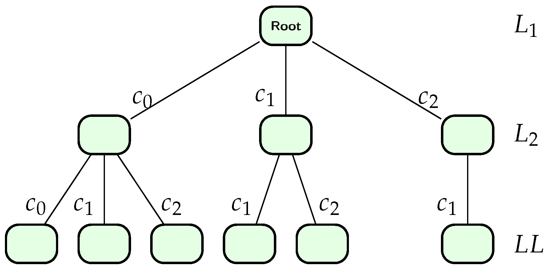
An example of a multiset-trie data structure with $\sigma =2$ and $\Sigma =I=\{1,2\}$ (i.e., the mapping $\varphi$ is an identity mapping) is shown in Figure 1. In the figure, which stores elements of $\{\varnothing ,\{1,1,2\},$$\{1,2,2\},$$\left\{2\right\},$$\{1,2\},$$\{2,2\}\}$, the degree of a node is set to be $n=3,$ so the maximal multiplicity of an element in a multiset is $n-1=2.$

Let a pair $(L_i,c_j)$ represent a node with label $c_j$ at a level $L_i.$ The pair $(L_1,c_j)$ is equivalent to $(L_1,root),$ since the first level has the root node only. According to Figure 1, we can extract the inserted multisets as follows:

$$\begin{array}{ccc}\hfill (L_1,root)\to (L_2,c_0)\to (LL,c_0)& =& \{1^0,2^0\}=\varnothing \hfill \\ \hfill (L_1,root)\to (L_2,c_0)\to (LL,c_1)& =& \{1^0,2^1\}=\left\{2\right\}\hfill \\ \hfill (L_1,root)\to (L_2,c_0)\to (LL,c_2)& =& \{1^0,2^2\}=\{2,2\}\hfill \\ \hfill (L_1,root)\to (L_2,c_1)\to (LL,c_1)& =& \{1^1,2^1\}=\{1,2\}\hfill \\ \hfill (L_1,root)\to (L_2,c_1)\to (LL,c_2)& =& \{1^1,2^2\}=\{1,2,2\}\hfill \\ \hfill (L_1,root)\to (L_2,c_2)\to (LL,c_1)& =& \{1^2,2^1\}=\{1,1,2\}\hfill \end{array}$$

where $e^k$ represents an element e with multiplicity $k.$

3. Multiset-Trie Operations

Let $\mathcal{M}$ be a multiset-trie and let M be a set of multisets that are inserted into the multiset-trie $\mathcal{M}.$ We define a type Multiset in order to use it as a representation of a multiset. The type Multiset is an array m of constant length $\sigma ,$ where the i-th cell represents the element ${\varphi }^{-1}\left(i\right)$ from $\Sigma$ with multiplicity $m\left[i\right].$ From now on, we agree that the first cell of an array has index 1. Let us give an example of a Multiset instance with $\sigma =2:$

The operations supported by the multiset-trie data structure are as follows.

• insert($\mathcal{M}$, m): inserts a multiset m into $\mathcal{M}$ if $m\notin M;$
• search($\mathcal{M}$, m): returns true if a multiset $m\in M$ for a given $\mathcal{M},$ and returns false otherwise;
• delete($\mathcal{M}$, m): returns true if a multiset m was successfully deleted from $\mathcal{M},$ and returns false otherwise (in case $m\notin M$);
• submsetExistence($\mathcal{M}$, m, $dev$): returns true if there exists a $x\in M$ for a given $\mathcal{M}$ such that $x\subseteq m$ and $\left|x\right[i]-m[i\left]\right|\le dev$ for $1\le i\le \sigma$, and returns false otherwise;
• supermsetExistence($\mathcal{M}$, m, $dev$): returns true if there exists a $x\in M$ for a given $\mathcal{M}$ such that $x\supseteq m$ and $\left|x\right[i]-m[i\left]\right|\le dev$ for $1\le i\le \sigma$, and returns false otherwise;
• getAllSubmsets($\mathcal{M}$, m, $dev$): returns the set of multisets $\{x\in M:x\subseteq m\wedge |x\left[i\right]-m\left[i\right]|\le dev\}$ for a given $\mathcal{M},$ where $1\le i\le \sigma ;$
• getAllSupermsets($\mathcal{M}$, m, $dev$): returns the set of multisets $\{x\in M:x\supseteq m\wedge |x\left[i\right]-m\left[i\right]|\le dev\}$ for a given $\mathcal{M},$ where $1\le i\le \sigma .$

The parameter $dev$ is used to specify the maximal deviation in the multiplicity of multiset containment operations. It is utilized to limit the search in multiset containment queries to the sub-multisets and super-multisets that are the closest to the input multiset m. In addition, we use $dev$ for the implementation of a multiset similarity search that, given m, retrieves from $\mathcal{M}$ all sub-multisets or super-multisets that are similar to m with respect to the deviation $dev$.

In the following subsections, we will present each operation of the multiset-trie data structure separately.

Firstly, we would like to describe some notations that will be used. The multiset-trie data structure is a recursive data structure. Hence, any subtree of a multiset-trie $\mathcal{M}$ is again a multiset-trie. This fact allows us to use the root node of a multiset-trie as its representative. Thus, the notation $\mathcal{M}$ will be used instead of $\mathcal{M}.root$ to refer to the root node of $\mathcal{M}.$ Non-existing or Null nodes in multiset-trie will be marked as Null and existing nodes at the level $LL$ will be marked as accepting nodes. The array slicing operation will be used as follows. For a given array $a,$$a[i:]$ represents the array obtained from a by taking only the cells from index i until the last cell.

3.1. Insert

The procedure insert($\mathcal{M}$, m) inserts a new instance m of type Multiset into multiset-trie $\mathcal{M}$. If the complete path already exists, then the procedure leaves the structure unchanged. Otherwise, it extends partially existing paths or creates a new complete path. The procedure does not return any result. The pseudocode for procedure insert is presented in Algorithm 1.

Algorithm 1: Procedure insert.

1: procedure insert($\mathcal{M}$, m) 2:     $currentNode\leftarrow \mathcal{M}$ 3:     for $i=1$ to $\sigma$ do 4:         if child $c_{m\left[i\right]}$ of $currentNode$ is Null then 5:            create new child $c_{m\left[i\right]}$ of $currentNode$ 6:         $currentNode\leftarrow c_{m\left[i\right]}$ 7:     mark $currentNode$ as accepting

3.2. Search

The function search($\mathcal{M}$, m) checks if the complete path corresponding to a given multiset m exists in the structure $\mathcal{M}.$ The function returns true if the multiset m exists in $\mathcal{M}$, and returns false otherwise. The function search is presented in Algorithm 2.

Algorithm 2: Function search.

1: function search($\mathcal{M}$, m) 2:     $currentNode\leftarrow \mathcal{M}$ 3:     for $i=1$ to $\sigma$ do 4:         if child $c_{m\left[i\right]}$ of $currentNode$ is Null then 5:            return False 6:         $currentNode\leftarrow c_{m\left[i\right]}$ 7:     return True

3.3. Delete

Function delete($\mathcal{M},$m) searches for the complete path that corresponds to m in order to remove it. If the path cannot be found, the function immediately returns false. During the search, the function keeps track of the number of children for every node. It marks the nodes that have more than one child as parent nodes and remembers the label of the child, which is a potential node where the subtree will be cut to remove the multiset. The parent node is needed to perform a removal because the multiset-trie is an explicit data structure. When the search is completed, the function removes the subtree of the last found parent node and returns true. In such a way, after deletion, all the prefixes for other multisets are preserved in $\mathcal{M}$ and m is removed. The function delete is presented in Algorithm 3.

Algorithm 3: Function delete.

1: function delete($\mathcal{M},$m) 2:     $currentNode\leftarrow \mathcal{M}$ 3:     $parent\leftarrow currentNode$ 4:     $position\leftarrow 1$ 5:     for $i=1$ to $\sigma$ do 6:         if child $c_{m\left[i\right]}$ of $currentNode$ is Null then 7:            return False 8:         $numChildren\leftarrow 0$ 9:         for $j=0$ to $n-1$ do 10:            if child $c_j$ of $currentNode$ is not Null then 11:                $numChildren\leftarrow numChildren+1$ 12:         if $numChildren$ is not 1 then 13:            $parent\leftarrow currentNode$ 14:            $position\leftarrow i$ 15:         $currentNode\leftarrow c_{m\left[i\right]}$ 16:     child $c_{m\left[position\right]}$ of $parent\leftarrow$ Null 17:     return True

3.4. Sub-Multiset and Super-Multiset Existence

The functions submsetExistence and supermsetExistence are symmetrical in the following sense. Let a multiset m represent the borderline in $\mathcal{M}$ defined by a path from the root to a leaf following the elements from m. The operation submsetExistence searches the left part of $\mathcal{M}$ and the operation supermsetExistence the right part of $\mathcal{M}$.

The function submsetExistence($\mathcal{M},m,dev$) checks if there exists a multiset x in $\mathcal{M},$ that satisfies the condition $x\subseteq m$ and $\left|x\right[i]-m[i\left]\right|\le dev,$ where $1\le i\le \sigma .$ The function starts with searching for an exact match $x=m$ in $\mathcal{M},$ since $m\subseteq m$ by definition of sub-multiset inclusion. If an exact match is not found in $\mathcal{M},$ the function uses multiset-trie to find the closest (the largest) sub-multiset of m in $\mathcal{M}$ by decreasing the multiplicity of elements in $m.$ The parameter $dev$ is used to limit a maximal deviation of multiplicity for a particular element in x with respect to $m.$ At every level, the function tries to proceed with the largest possible multiplicity of an element that is provided by $m.$ However, when the function reaches some level where it meets a Null node and cannot go further using the path provided by $m,$ it decreases the multiplicity of an element that corresponds to a current level with respect to the specified maximal deviation. Thus, the function can decrease the multiplicity of an element or eventually skip it in order to find the closest $x\subseteq m.$ The function submsetExistence is presented in Algorithm 4.

Algorithm 4: Function submsetExistence.

1: function submsetExistence($\mathcal{M},m,dev$) 2:     $currentNode\leftarrow \mathcal{M}$ 3:     if $currentNode$ is accepting then 4:         return True 5:     for $i=m\left[1\right]$ down to max($0,m\left[1\right]-dev$) do 6:         if child $c_i$ of $currentNode$ is not Null then 7:            if submsetExistence($c_i,m[2:],dev$) then 8:                return True 9:     return False

The function supermsetExistence($\mathcal{M},m,dev$) checks if there exists super-multiset x of a given multiset m in $\mathcal{M},$ such that condition $\left|x\right[i]-m[i\left]\right|\le dev$ is satisfied, where $1\le i\le \sigma .$ Symmetrically to the function submsetExistence, the function supermsetExistence searches first for an exact match $x=m$ in $\mathcal{M}.$ If such x does not exist in $\mathcal{M},$ then the function searches on the right side of the borderline representing an exact match of m in $\mathcal{M}.$ Since we would like to find the closest (the smallest) super-multiset, we increase the multiplicity of elements in m at every level of $\left(M\right)$ starting with the multiplicities of $m.$ The function supermsetExistence is presented in Algorithm 5.

Algorithm 5: Function supermsetExistence.

1: function supermsetExistence($\mathcal{M},m,dev$) 2:     $currentNode\leftarrow \mathcal{M}$ 3:     if $currentNode$ is accepting then 4:         return True 5:     for $i=m\left[1\right]$ to min($n-1,m\left[1\right]+dev$) do 6:         if child $c_i$ of $currentNode$ is not Null then 7:            if supermsetExistence($c_i,$$m[2:],dev$) then 8:                return True 9:     return False

3.5. Get All Sub-Multisets and Get All Super-Multisets

The algorithms for functions getAllSubmsets and getAllSupermsets are based entirely on algorithms for submsetExistence and supermsetExistence functions that do not terminate on the first existing sub/super-multiset, but store the results and continue the procedure until all existing sub/super-multisets in $\mathcal{M}$ are found and stored. The functions getAllSubmsets and getAllSupermsets are presented in Algorithms 6 and 7, respectively.

In order to record a multiset during multiset-trie traversal, we use the variable x in the algorithms. It is an empty array of size $\sigma$ where we store multiplicities of elements at each level as we traverse the tree. The variable $result$ is used as a container for storing sub-multisets of m found during traversal. Both variables x and $result$ are presented as global; however, they could be passed to the recursive function as parameters.

Algorithm 6: Function getAllSubmsets.

1: $result\leftarrow$ empty container 2: $x\leftarrow$ empty array of size $\sigma$ 3: function getAllSubmsets($\mathcal{M},m,dev$) 4:     $currentNode\leftarrow \mathcal{M}$ 5:     if $currentNode$ is accepting then 6:         add copy of x to $result$ 7:     for $i=m\left[1\right]$ down to max($0,m\left[1\right]-dev$) do 8:         if child $c_i$ of $currentNode$ is not Null then 9:            $x\left[1\right]\leftarrow i$ 10:          getAllSubmsets($c_i,m[2:],dev$)

Algorithm 7: Function getAllSupermsets.

1: $result\leftarrow$ empty container 2: $x\leftarrow$ empty array of size $\sigma$ 3: function getAllSupermsets($\mathcal{M},m,dev$) 4:     $currentNode\leftarrow \mathcal{M}$ 5:     if $currentNode$ is accepting then 6:         add copy of x to $result$ 7:     for $i=m\left[1\right]$ to min($n-1,m\left[1\right]+dev$) do 8:         if child $c_i$ of $currentNode$ is not Null then 9:            $x\left[1\right]\leftarrow i$ getAllSupermsets($c_i,$$m[2:],dev$)

4. Mathematical Analysis of the Structure

In this section, we present theoretical results of the time and space complexity of the multiset-trie data structure. In the following Section 4.1, we discuss the running time complexity of the presented algorithms. First, in Section 4.1.1, we present the mathematical model that we use to describe the distribution of multisets in the multiset-trie and input data. Using a probabilistic approach and tools from a Galton–Watson process, we measure the expected cardinality of the multiset-trie in Theorem 2. Further, we derive the expected cardinality of the searched subtree of the multiset-trie parametrized by an input multiset in Corollary 1.

In Section 4.1.2, we discuss the running time complexity of the functions getAllSubmsets and getAllSupermsets. We observe that the complexity of the functions is exponential. Moreover, the worst-case running time complexity is the same for both functions, and its upper bound is the cardinality of the multiset-trie.

The remaining “existence” functions are discussed in Section 4.1.3. We observe that, beyond the scope of our mathematical model, unlike in functions getAllSubmsets and getAllSupermsets, the mapping $\varphi$ has an impact on the performance of the functions submsetExistence and supermsetExistence. In particular, the frequency analysis of the symbols from $\Sigma$ in input data determines such a $\varphi$ that gives a boost in performance.

We find that the performance of the functions submsetExistence and supermsetExistence in the worst-case scenario is also proportional to the size of the constructed trie. We give a rather technical upper bound for the worst-case running time complexity, which appears to be the same for both functions. However, it must be stressed that for the positive outcome, this worst-case behavior holds only on specific cases, such as the presence of the empty set in the multiset-trie.

Finalizing the mathematical analysis, we present the study of the space complexity of the multiset-trie in Section 4.2. We show that the space used for the storage is asymptotically equal to the size of the input data.

4.1. Time Complexity of the Algorithms

The performance of the functions will be measured by the number of visited nodes in a multiset-trie during the execution of a particular query by the functions search, delete, submsetExistence, supermsetExistence, getAllSubmsets, getAllSupermsets and the procedure insert.

By the design of the multiset-trie, it is easy to see that the functions search, delete and the procedure insert have complexity of $O\left(\sigma \right).$ Because $\sigma$ is defined when the structure is initialized and does not depend on the user input afterwards, the asymptotic complexity of the functions search, delete and the procedure insert is $O\left(1\right).$ Nonetheless, in the general case, the complexity is $O\left(\sigma \right).$

In what follows, we focus on the analysis of the more involved functions: submsetExistence, supermsetExistence, getAllSubmsets, and getAllSupermsets.

4.1.1. Mathematical Model

We start with the basics of our mathematical model. Let $\Sigma$ be an alphabet of cardinality $\sigma ,$ such that $\Sigma =\{1,2,\dots ,\sigma \}.$ Define N to be the set of all possible multisets that can be inserted in a multiset-trie. Let n be the maximal degree of a node in a multiset-trie. Then, the maximal multiplicity of an element in a multiset is equal to $n-1.$ Thus, the number of multisets in a complete multiset-trie is $\left|N\right|=n^{\sigma }.$ Let M be a collection of multisets inserted into multiset-trie $\mathcal{M}.$ All the multisets in M are constructed from the alphabet $\Sigma$ according to the parameters $\sigma$ and n. Hence, any multiset $m\in M,$ has at most $\sigma$ distinct elements that are members of $\Sigma$, and every distinct element in m has multiplicity strictly less than $n.$ Because a multiset does not distinguish different orderings, it is assumed, for simplicity, that all elements are ordered in ascending order. A multiset m is represented as $\{1^{k_1},2^{k_2},\dots ,{\sigma }^{k_{\sigma }}\},$ where $e^{k_e}$ represents an element $e\in \Sigma$ with multiplicity $k_e.$

Denote the nodes of multiset-trie on all levels but on $\sigma +1$ as internal and nodes on the leaf level as leaf nodes. Observe that every internal non-root node has a degree of at least 1. Indeed, the insertion of a multiset requires the construction of a path of length $\sigma +1,$ meaning that if an internal node exists in a multiset-trie, it must have a degree of at least 1. It also follows that the height of a multiset-trie is always $\sigma +1$ as soon as at least one multiset is inserted into the data structure.

Our model assumes that all the inserted multisets are chosen with the same probability, meaning that for some $p\in (0,1)$, the following holds:

$$P(m\in M)=p,\forall m\in N.$$

Let ${\xi }_1,{\xi }_2,\dots ,{\xi }_{\sigma +1}$ be random variables such that ${\xi }_i$ represents the number of nodes in a multiset-trie on the i-th level. For every node j on i-th level, we assign a random variable ${\xi }_{ij}$ to be the number of its children, such that $j\in [1,{\xi }_i].$ Then, for every $i\in [1,\sigma ]$, the following holds:

$${\xi }_{i+1}=\sum _{j=1}^{{\xi }_i}{\xi }_{ij},$$

(1)

where ${\xi }_1=1.$ It is easy to see that the variable ${\xi }_{i+1}$ can have values in the interval $[{\xi }_i,n^i]$ and the value of the variable ${\xi }_{ij}$ is within the interval $[1,n].$ Without conditioning on the existence of any node in multiset-trie, it is easy to describe the probability of the existence of any individual node.

Lemma 1.

Any potential node on a fixed level $i,$ where $i\in \{1,2,\dots ,\sigma +1\}$ exists, with probability

$$p_i=1-{(1-p)}^{n^{\sigma +1-i}}.$$

(2)

Proof. 

Let v be an arbitrary node in a multiset-trie on an arbitrary level $i.$ Consider the subtree with the root v and call it the v-subtree. Since the height of the multiset-trie is $\sigma +1$, we can calculate the height of the v-subtree. Taking into account that the root node has height 1, the height of the v-subtree is

$$h_v=\sigma +1-i.$$

A node in a multiset-trie exists if at least one node exists on the leaf level of its subtree, i.e., a node on the level $\sigma +1$ that belongs to v-subtree. The possible number of nodes on the leaf level of v-subtree can be easily calculated knowing its height. It is equal to

$$n^{\sigma +1-i}.$$

A node at level $\sigma +1$ exists with probability $p,$ where $p=P(m\in M).$ Thus, the probability that there are no nodes on the leaf level in v-subtree is

$${(1-p)}^{n^{\sigma +1-i}}.$$

The claim follows by taking the complement probability of the above result. □

Recall that for any given discrete random variable X taking values over positive non-negative integral values, one can define a so-called probability generating function (PGF, for short) $G_X$ to be a formal power series defined as

$$\begin{array}{c}\hfill G_X\left(z\right)=\sum _{i\ge 0}Pr(X=i)z^i.\end{array}$$

While the PGFs are usually not meant to be evaluated for concrete values of z, certain values have special interpretation when used in PGF, or in a derivation(s) of PGF. For instance, $Pr(X=0)=G_X\left(0\right)$, and also $\mathbb{E}\left(X\right)=G_X^{\prime }\left(1\right)$. For many values of z, the function $G_X$ may not converge to any finite value. For this reason, it is a common notation to write, in particular,

$$G_X\left(1^{-}\right)=\underset{z\nearrow 1}{lim}{G}_X\left(z\right).$$

In what follows, we will denote a Bernoulli-distributed random variable with parameter p as $Bernoulli\left(p\right)$. Furthermore, we denote a zero-truncated binomially distributed random variable on parameters n and $p_{i+1}$ by ${\mathcal{B}}_0(n,p_{i+1})$. Finally, $\stackrel{d}{=}$ indicates so-called equality in distribution.

Example 1.

The probability generating function of a binomial random variable $\mathcal{B}(n,p)$, the number of successes in n trials, with probability p of success in each trial, is

$$\begin{array}{cc}\hfill G_{\mathcal{B}(n,p)}\left(z\right)=G\left(z\right)& =\sum _{k=0}^n\left(\genfrac{}{}{0pt}{}{n}{k}\right)p^k{(1-p)}^{n-k}{z}^k\hfill \\ \hfill & =\sum _{k=0}^n\left(\genfrac{}{}{0pt}{}{n}{k}\right){\left(pz\right)}^k{(1-p)}^{n-k}\hfill \\ \hfill & ={\left((1-p)+pz\right)}^n.\hfill \end{array}$$

It is thus easy to compute expectation

$$\mathbb{E}\left(\mathcal{B}(n,p)\right)=G^{\prime }\left(1\right)=np.$$

We now focus our attention on the distribution of ${\xi }_{ij}$.

Lemma 2.

Suppose that a node v exists at level $1\le i\le \sigma$. Then, the number of its children ${\xi }_{iv}$ is modeled by a zero-truncated binomially distributed random variable on parameters n and $p_{i+1}$. In particular, the probability of node v having k children equals

$$P({\xi }_{iv}=k)=\frac{\left(\genfrac{}{}{0pt}{}{n}{k}\right){(1-p_{i+1})}^{n-k}}{1-{(1-p_{i+1})}^n}$$

(3)

and the corresponding probability generating function equals

$${\mathcal{B}}_0(n,p_{i+1})\stackrel{d}{=}{G}_i\left(z\right)=\frac{{(1+p_{i+1}(z-1))}^n-{(1-p_{i+1})}^n}{1-{(1-p_{i+1})}^n}.$$

(4)

Proof. 

In order to prove the lemma, we have to show that ${\xi }_{iv}\stackrel{d}{=}{\mathcal{B}}_0(n,p_{i+1}).$ Consider an arbitrary node v on level $1\le i\le \sigma .$ According to the definition of the multiset-trie, a node exists at level i if and only if it has at least one child. Note that this is not true for the nodes on the leaf level $\sigma +1.$ This implies that a node on level i can have $k\in \{1,2,\dots ,n\}$ children. Let $X_0,X_1,\dots ,X_{n-1}$ be random variables; they are defined as follows:

$$X_k=\left\{\begin{array}{cc}0\hfill & \mathrm{child}k\mathrm{of}\mathrm{node}v\mathrm{does}\mathrm{not}\mathrm{exist}\hfill \\ 1\hfill & \mathrm{child}k\mathrm{of}\mathrm{node}v\mathrm{exists}\hfill \end{array}\right.$$

As was shown in the previous Lemma 2, the distribution of $X_k$ is $X_k\stackrel{d}{=}Bernoulli\left(p_{i+1}\right).$ Since our model assumes that all the multisets in M are chosen uniformly at random, the variables $X_k,X_l$ are independent for $k\ne l.$ However, in our case, the node v cannot have 0 children, so the sum ${\sum }_{k=1}^n{X}_k$ has a zero-truncated binomial distribution,

$$\sum _{k=1}^n{X}_k\stackrel{d}{=}{\mathcal{B}}_0(n,p_{i+1}),$$

which completes the proof. □

Knowing the probability density and probability generating functions of ${\xi }_{ij}$ from Lemma 2, we can now estimate the number of nodes in a randomly generated multiset-trie as follows:

$$\mathbb{E}\left(\right|\mathcal{M}\left|\right)=\mathbb{E}\left[\sum _{i=1}^{\sigma +1}{\xi }_i\right].$$

(5)

In order to evaluate (5), we will use some of the tools from a Galton–Watson process; see Gardiner [26] for an introduction. Using Equations (1) and (4), we can derive the probability generating function for the random variable ${\xi }_{i+1}$ as

$$G_{{\xi }_{i+1}}\left(z\right)=G_{{\xi }_i}\left(G_i\left(z\right)\right).$$

(6)

Since there is always precisely one node at the root level, we have $P({\xi }_1=1)=1.$ Hence, the probability generating function for the random variable ${\xi }_1$ is

$$G_{{\xi }_1}\left(z\right)=z^1=z$$

(7)

which is the initial condition for the recursive Equation (6).

Proposition 1.

The expectation of the random variable ${\xi }_{i+1}$ can be expressed as follows.

$$\mathbb{E}\left({\xi }_{i+1}\right)=\mathbb{E}\left({\xi }_i\right)\mathbb{E}\left({\mathcal{B}}_0(n,p_{i+1})\right)$$

for $1\le i\le \sigma .$

Proof. 

Using the following property of probability generating function

$$G_X^{\prime }\left(1^{-}\right)=\mathbb{E}\left(X\right)$$

(8)

the expectation for the random variable ${\xi }_{i+1}$ can be derived in terms of Equation (6).

$$\begin{array}{ccc}\hfill \mathbb{E}\left({\xi }_{i+1}\right)& =& G_{{\xi }_{i+1}}^{\prime }\left(1^{-}\right)\hfill \\ & =& G_{{\xi }_i}^{\prime }\left(G_i\left(1^{-}\right)\right)G_i^{\prime }\left(1^{-}\right).\hfill \end{array}$$

(9)

According to (3) and (4), the value of $G_i\left(z\right)$ at 1 is 1 and the value of its derivative at 1 is $\mathbb{E}\left({\mathcal{B}}_0(n,p_{i+1})\right).$ Substituting the values of $G_i\left(1^{-}\right)$ and $G_i^{\prime }\left(1^{-}\right),$ and applying the property (8), we complete the proof. □

From Proposition 1 above and Lemma 2, we can conclude that

$$\begin{array}{ccc}\hfill \mathbb{E}\left({\xi }_i\right)& =& \mathbb{E}\left({\xi }_{i-1}\right)\mathbb{E}\left({\mathcal{B}}_0(n,p_i)\right)\hfill \\ & =& \mathbb{E}\left({\xi }_{i-1}\right)\frac{n{p}_i}{1-{(1-p_i)}^n}.\hfill \end{array}$$

(10)

Theorem 1.

Let $\mathcal{M}$ be a multiset-trie defined with parameters $n,$$\sigma ,$ and denote the number of nodes on every level i by a random variable ${\xi }_i.$ Furthermore, let all multisets appear in $\mathcal{M}$ with equal probability $p\in (0,1).$ Then, the expected number of nodes on every level of $\mathcal{M},$ i.e., $\mathbb{E}\left({\xi }_i\right)$, is defined as

$$\mathbb{E}\left({\xi }_i\right)=n^{i-1}\frac{1-{(1-p)}^{n^{\sigma +1-i}}}{1-{(1-p)}^{n^{\sigma }}}.$$

(11)

Proof. 

According to (7), the expected number of nodes on the first level is 1.

Using $\mathbb{E}\left({\xi }_1\right)=1$ and the result from Proposition 1, we obtain

$$\begin{array}{cc}\hfill \mathbb{E}\left({\xi }_i\right)& =\prod _{j=2}^i\frac{n{p}_j}{1-{(1-p_j)}^n}=\prod _{j=2}^{i}n\frac{1-{(1-p)}^{n^{\sigma +1-j}}}{1-{(1-p)}^{n^{\sigma +2-j}}}\hfill \\ \hfill & =n^{i-1}\frac{1-{(1-p)}^{n^{\sigma +1-i}}}{1-{(1-p)}^{n^{\sigma }}}\hfill \end{array}$$

□

Having derived the expected number of nodes on every level of multiset-trie, the expected value of the total number of nodes in a multiset-trie can be calculated with respect to the parameters $n,$ $\sigma$ and $p.$ This result is obtained in the next theorem.

Theorem 2.

The expected cardinality of a multiset-trie defined on parameters $n,$ σ, and p can be computed as

$$\mathbb{E}\left(\right|\mathcal{M}\left|\right)=\sum _{i=1}^{\sigma +1}{n}^{i-1}\frac{1-{(1-p)}^{n^{\sigma +1-i}}}{1-{(1-p)}^{n^{\sigma }}},$$

(12)

where $r={(1-p)}^n,$ so $r\in (0,1).$

Proof. 

Using the results obtained from Theorem 1, we compute

$$\begin{array}{cc}\hfill \mathbb{E}\left(\right|\mathcal{M}\left|\right)& =\mathbb{E}\left[\sum _{i=1}^{\sigma +1}{\xi }_i\right]\hfill \\ \hfill & =\sum _{i=1}^{\sigma +1}{n}^{i-1}\frac{1-{(1-p)}^{n^{\sigma +1-i}}}{1-{(1-p)}^{n^{\sigma }}}\hfill \end{array}$$

□

With the expected number of nodes in a multiset-trie $\mathcal{M}$ obtained from Theorem 2, we can now generalize the result for a subtree in $\mathcal{M}$ parametrized by an input multiset $m.$ The subtrees that we are interested in are the ones that contain all the sub-multisets or all the super-multisets of $m.$ In order to calculate the expected cardinality of such subtrees, we need the following definition.

Definition 1.

Let $m=\{1^{k_1},2^{k_2},\dots ,{\sigma }^{k_{\sigma }}\},$ where $e^{k_e}$ is an element e with multiplicity $k_e.$ Let $M_1,M_2$ be the subsets of the set $M,$ such that $M_1=\{x\in M:x\subseteq m\}$ and $M_2=\{x\in M:x\supseteq m\}.$ Define ${\alpha }_i$ and ${\beta }_i$ as follows:

$${\alpha }_i=\left\{\begin{array}{cc}1,\hfill & i=0\hfill \\ \prod _{j=1}^i(k_j+1),\hfill & 1\le i\le \sigma \hfill \end{array}\right.$$

and

$${\beta }_i=\left\{\begin{array}{cc}1,\hfill & i=0\hfill \\ \prod _{j=1}^i(n-k_j-1),\hfill & 1\le i\le \sigma \hfill \end{array}\right..$$

The expected cardinality of the subtrees containing the multisets from $M_1$ or $M_2$ is defined in the following corollary.

Corollary 1.

Let $M_1,M_2,{\alpha }_i$ and ${\beta }_i$ be defined as in Definition 1; then, the expected cardinality of a multiset-trie subtree ${\mathcal{M}}_{M_1}$ that contains all the multisets from the set $M_1$ is equal to

$$\mathbb{E}\left(\right|{\mathcal{M}}_{M_1}\left|\right)=\sum _{i=1}^{\sigma +1}{\alpha }_{i-1}\frac{1-{(1-p)}^{{\alpha }_{i-1}}}{1-{(1-p)}^{{\alpha }_{\sigma }}}.$$

(13)

The expected cardinality of a multiset-trie subtree ${\mathcal{M}}_{M_2}$ that contains all the multisets from the set $M_2$ is equal to

$$\mathbb{E}\left(\right|{\mathcal{M}}_{M_2}\left|\right)=\sum _{i=1}^{\sigma +1}{\beta }_{i-1}\frac{1-{(1-p)}^{{\beta }_{i-1}}}{1-{(1-p)}^{{\beta }_{\sigma }}}.$$

(14)

Proof. 

Using the results from Theorems 1 and 2, we derive the formulas (13) and (14) by specifying the possible number of nodes on every level in the multiset-trie according to the multiset $m.$ Note that the formula (11) assumes that, on every level but the first one, there are n possible nodes. Given a sub-multiset or super-multiset query and an input multiset m, the number of nodes that will be traversed on level i is defined by the number $k_{i-1}+1$ or $n-k_{i-1}-1$ for $i\ge 2.$ On level $i=1$, there is only one root node in any multiset-trie $\mathcal{M},$ which always exists if $M\ne \varnothing$ and is traversed for any type of query (sub-multiset and super-multiset). □

4.1.2. GetAllSubmsets and GetAllSupermsets

In this subsection, we discuss the running time complexity of the functions getAllSubmsets and getAllSupermsets. It is obvious that any other algorithm for retrieving all the sub-multisets or super-multisets has a worst-case running time complexity of at least $O\left(\right|M\left|\right).$ Hence, the functions getAllSubmsets and getAllSupermsets have the worst-case running time complexity $O\left(\right|\mathcal{M}\left|\right).$ Indeed, the case when the algorithms retrieve all the multisets stored in a multiset-trie by traversing the whole structure can be easily constructed.

Consider the function getAllSubmsets. The function takes some multiset m as an input argument. Then, it returns a set of multisets $\{x\in M:x\subseteq m\}$ from the multiset-trie $\mathcal{M}$. Having a multiset m set to the largest possible multiset in N (it can also be larger),

$$m=\{1^{n-1},2^{n-1},\dots ,{\sigma }^{n-1}\}$$

the whole multiset-trie is traversed during the getAllSubmsets query.

Now, let us consider the function getAllSupermsets. Similarly, the function takes a multiset m as an input argument. However, in this case, it returns the set of multisets $\{x\in M:x\supseteq m\}$ from the multiset-trie $\mathcal{M}.$ In order to obtain the traversing of all the multiset-trie, one must set m to the smallest possible multiset, i.e., an empty multiset

$$m=\{\varnothing \}=\{1^0,2^0,\dots ,{\sigma }^0\}.$$

Thus, we can conclude that the worst-case running time complexity of the functions getAllSubmsets and getAllSupermsets is $O\left(\mathbb{E}\right(\left|\mathcal{M}\right|\left)\right).$ According to Theorem 2, the expected number of visited nodes in the worst case is

$$O(\sum _{i=1}^{\sigma +1}{n}^{i-1}\frac{1-{(1-p)}^{n^{\sigma +1-i}}}{1-{(1-p)}^{n^{\sigma }}}).$$

According to Theorem 1, the worst-case running time complexity given an input multiset m for the function getAllSubmsets is

$$O(\sum _{i=1}^{\sigma +1}{\alpha }_{i-1}\frac{1-{(1-p)}^{{\alpha }_{i-1}}}{1-{(1-p)}^{{\alpha }_{\sigma }}})$$

and for the function getAllSupermsets is

$$O(\sum _{i=1}^{\sigma +1}{\beta }_{i-1}\frac{1-{(1-p)}^{{\beta }_{i-1}}}{1-{(1-p)}^{{\beta }_{\sigma }}}).$$

4.1.3. SubmsetExistence and SupermsetExistence

We start the analysis of the functions submsetExistence and supermsetExistence with an observation. Our theoretical model assumes that all the multisets are inserted into multiset-trie at random. It was already concluded that the probability distribution function $P(m\in M)$ has an impact on the size of multiset-trie $\mathcal{M}.$ Moreover, this distribution influences the performance of the functions submsetExistence and supermsetExistence even more.

For a real-world model, such that $P(m\in M)\ne const$, the performance of the search algorithms directly depends on the number of nodes on every level ${\xi }_i.$ When the search functions check if a multiset is in multiset-trie, the complete path that corresponds to this multiset is checked. Knowing this fact, the search can be optimized during the construction of a multiset-trie.

Recall that a multiset-trie is defined on parameters $n,$$\Sigma ,$$\sigma =|\Sigma |$, and $\varphi .$ Let the frequency of an element e in a multiset m be the multiplicity of e in $m,$ denoted by $mul{t}_m\left(e\right).$ Then, the frequency of an element e can be defined as a sum ${\sum }_{m\in M}mul{t}_m\left(e\right).$ According to the frequencies of elements in $\Sigma ,$ the performance of the multiset-trie can be optimized by the mapping $\varphi :\Sigma \to I.$ Indeed, the ordering of elements by their frequencies has an influence on the performance. The frequency of an element $e\in \Sigma$ affects the distribution of ${\xi }_{\varphi \left(e\right)}$ as follows. The larger the frequency of e, the larger the number of nodes on the $\varphi \left(e\right)$ level. Thus, if the number of nodes on lower levels is greater than on higher levels, then the search functions will discard complete paths that do not satisfy the query faster. Hence, the closest match will be found faster.

Let us now switch back to our mathematical model and note that the influence of the mapping function $\varphi$ in our model has an inessential impact on the performance, because all the multisets are equally likely, and the whole domain N is used for sampling multisets.

Consider both functions submsetExistence and supermsetExistence. Whenever the result is false, i.e., no multiset in M is a sub-multiset or super-multiset of an input multiset $m,$ both functions in the worst case visit all the nodes in $\mathcal{M}$ but the nodes on the leaf level. Of course, such a case would be very rare, assuming a random input model, but it can be constructed as follows.

Consider the function submsetExistence. Then, given an input multiset $m=\{1^{k_1},2^{k_2},\dots ,{\sigma }^{k_{\sigma }}\},$ the collection of inserted multisets M must be equal to $M=\{x\in M:k_{x,\sigma }>k_{m,\sigma }\}.$ Analogically, for the function supermsetExistence with an input multiset $m=\{1^{k_1},2^{k_2},\dots ,{\sigma }^{k_{\sigma }}\},$ the collection of inserted multisets M must be equal to $M=\{x\in M:k_{x,\sigma }<k_{m,\sigma }\}.$

Thus, the worst-case running time complexity of the functions submsetExistence and supermsetExistence is $O\left(\right|\mathcal{M}|-|M\left|\right).$ According to Theorem 2, this value is

$$O(\sum _{i=1}^{\sigma }{n}^{i-1}\frac{1-{(1-p)}^{n^{\sigma +1-i}}}{1-{(1-p)}^{n^{\sigma }}}).$$

According to Theorem 1, the worst-case running time given an input multiset m for the function submsetExistence is

$$O(\sum _{i=1}^{\sigma }{\alpha }_{i-1}\frac{1-{(1-p)}^{{\alpha }_{i-1}}}{1-{(1-p)}^{{\alpha }_{\sigma }}})$$

and for the function supermsetExistence is

$$O(\sum _{i=1}^{\sigma }{\beta }_{i-1}\frac{1-{(1-p)}^{{\beta }_{i-1}}}{1-{(1-p)}^{{\beta }_{\sigma }}}).$$

Note that the summation goes only up to $\sigma$ and not up to $\sigma +1$ as in Theorem 2 or in Theorem 1.

As for the case wherein the outcome of the functions submsetExistence and supermsetExistence is true, one has to guarantee the termination of the algorithm at some node on the leaf level. The worst-case scenario can be constructed in the same way as for the false outcome but with two more multisets in $M.$ The first multiset is the empty multiset. With the empty multiset, the function submsetExistence will visit the same amount of nodes as for the false case, plus one more for the empty multiset. The second multiset is the maximal possible multiset from $N.$ In this case, the function supermsetExistence will also visit the same amount of nodes as for the false case, plus one more for the maximal multiset. Hence, the worst-case running time complexity for both outcomes (true and false) is the same.

4.2. Space Complexity

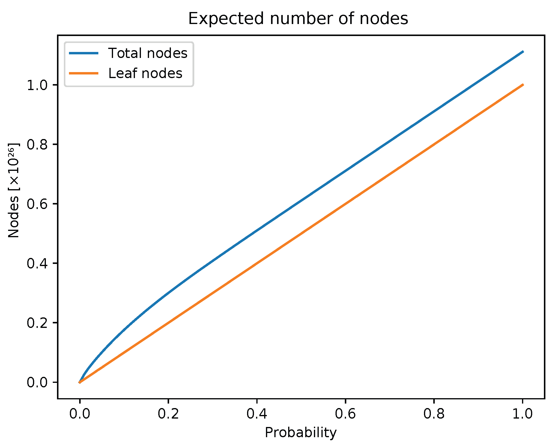
As in any efficient algorithm, there is always some trade-off between space and time complexity. While offering efficient sub- and super-multiset queries, an additional space must be provided for multiset storage. As we increase the parameter p, the number of sets we need to store (i.e., number of leaves) increases linearly. Figure 2 shows that the additional overhead space that our data structure uses does not increase as the tree is becoming more and more dense.

As we see in Figure 2, the value of $\left|\mathcal{M}\right|$ is slightly shifted with respect to the value of $\left|M\right|.$

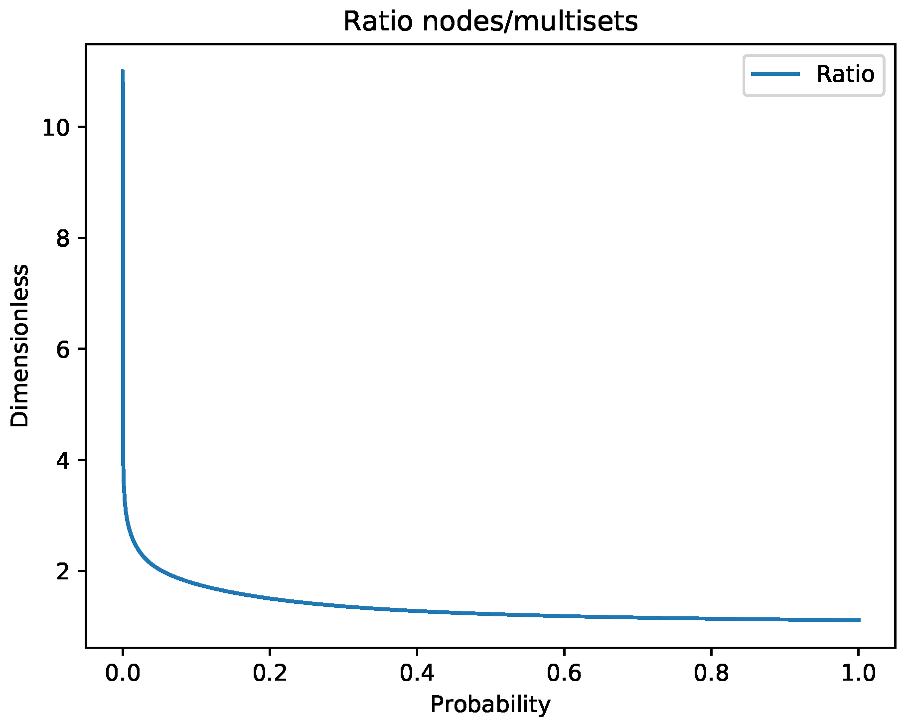
Now, we demonstrate a more descriptive comparison between $\left|\mathcal{M}\right|$ and $\left|M\right|.$ Figure 3 shows the ratio between the expected cardinality of a multiset-trie $\left|\mathcal{M}\right|$ and the actual number of multisets stored $\left|M\right|$ for parameters n and $\sigma$ being 10 and 26, respectively.

Analyzing the graph in Figure 3, we can safely say that the upper bound for the ratio is $\sigma +1.$ The argument holds because of the limit

$$\underset{p\to 0^{+}}{lim}\mathbb{E}\left({\xi }_i\right)=1,$$

(15)

where ${\xi }_i$ is the number of nodes on the i-th level and $1\le i\le \sigma +1.$

However, the ratio $\sigma +1$ can be obtained only with a very small cardinality of the set $M,$ in particular $\left|M\right|=1.$ In order to obtain such a case, the probability p must be at most $\frac{1}{n^{\sigma }}.$

The lower bound for the ratio is obviously at $p=1$ and is equal to 1:

$$\underset{n,\sigma \to \infty }{lim}\frac{n^{\sigma +1}-1}{n^{\sigma }(n-1)}=1.$$

(16)

Since the ratio $\sigma +1$ can be obtained for a very specific case only and with a small increase in probability, the ratio drops rapidly and it can be concluded that the space complexity of the multiset-trie is $O\left(\right|M\left|\right).$

4.3. An Informal Comment on the Mathematical Analysis

In the next section, we show how our data structure preforms in certain environments. We will see, in our view, great results throughout various experiments, even when compared with state-of-the-art approaches such as Inverted Index.

It was very frustrating to us that, despite these indications, it seems that this structure is very difficult to analyze. Even after restricting the analysis to the (usually simple) case wherein the input data are uniformly distributed, and after utilizing reliable probabilistic tools, our approach unfortunately did not provide as clear results as we hoped for. We would be very keen to learn of an approach or technique that would offer more insight into the mathematical analysis of our data structure and its algorithms.

5. Experiments

This section contains the results of experiments that were performed on the multiset-trie data structure. In particular, we tested the functions submsetExistence, supermsetExistence, getAllSubmsets, and getAllSupermsets. We refer to the former two operations as the existence operations, and the later two as the exhaustive operations.

The multiset-trie is implemented in the C++ programming language. The current implementation uses only the standard library of the C++14 version of the standard and has a command line interface [27]. The implementation of the program was optimized for testing, and, therefore, the program operates with files to process queries. After processing all the queries, the results are stored in files for further analysis.

The current implementation of multiset-trie is not optimized for space consumption. A node in the multiset-trie is implemented as a record indicating the level of the tree that corresponds to a symbol from $\Sigma$, and including an array of pointers to its children indexed by the multiplicities of the child symbols. The arrays have fixed length n from the interval $[0,n].$ Only some elements of an array may point to a child node, while others include a $Null$ value.

Before we start, we will give a few definitions of the parameters that were varied throughout the experiments and discuss the experimental data that were used.

Let M be a set of multisets inserted into multiset-trie and let n be the maximal node degree. Let N be the power multiset of $\Sigma ,$ where the multiplicity of each element is bounded from above by $n-1.$ We define the density of a multiset-trie to be the ratio $\frac{\left|M\right|}{\left|N\right|},$ where $|·|$ denotes cardinality.

The selected parameters of the data structure that were varied in the experiments were as follows:

• $\sigma$—the cardinality of the alphabet $\Sigma ;$
• n—the maximal degree of a node, which explicitly defines the maximal multiplicity of elements in a multiset;
• $\varphi$—mapping of letters from $\Sigma$ into a set of consecutive integers;
• d—density of a multiset-trie.

The cardinality of a power multiset N is equal to $n^{\sigma },$ which means that density d of a multiset-trie depends on parameters $\left|M\right|,$$\sigma$ and $n.$ Because parameters $\sigma$ and n are set when a multiset-trie is initialized, the parameter $\left|M\right|$ was varied to change the density in the experiments. As we mentioned in Section 2, the mapping $\varphi$ determines the correspondence of letters to levels in multiset-trie, i.e., it defines the ordering of levels in multiset-trie. It is also true that $\varphi$ defines the ordering in multisets.

In the following Section 1, Section 2, Section 3, Section 4 and Section 5, we will present the behavior of the multiset-trie data structure depending on the selected parameters, as well as the comparative benchmark of the multiset-trie against the B-tree implementation of Inverted Index. We start with experiments that were performed on artificially generated data in order to give a general picture of the multiset-trie’s performance.

In Experiment 1, a special case of the multiset-trie is considered. Only sets are allowed to be stored in the data structure, i.e., the maximally allowed multiplicity is set to 1. The performance is measured with respect to the density of the multiset-trie.

Experiment 2 was an extension of the previous one. Here, we also measured the performance of the multiset-trie depending on its density. The difference was that the allowed multiplicity of an element was raised, i.e., the data structure was populated with multisets.

Summarizing the tests of the performance depending on the density, we present Experiment 3. It shows the nonlinearity of the performance with respect to the density of the multiset-trie.

The fourth experiment on the multiset-trie uses real-world data. In Experiment 4, the influence of the mapping $\varphi$ is studied. The input data are obtained by mapping real words from the English dictionary to the set of consecutive integers using the function $\varphi .$ The experiment shows that the performance of the multiset-trie is noticeably influenced by different mappings $\varphi .$ It also shows the usability of the multiset-trie in terms of real data, demonstrating the high performance of search queries.

Finally, the empirical comparison of the multiset-trie data structure with the B-tree-based Inverted Index is presented in Experiment 5. We use Inverted Index to store and retrieve multisets in the same way as is described in the paper by Helmer and Moerkotte [23] for sets. In the comparison, we use three types of queries: exact, sub-multiset, and super-multiset retrieval.

5.1. Data Generation

We denote by input data the data that are used to fill the structure prior to testing and by test data the set of queries that are used to test the performance of the functions.

The artificially generated input data are obtained by sampling $\left|M\right|$ multisets from $N.$ All the multisets in N are constructed according to parameters $\sigma$ and n and represent the power multiset of the alphabet $\Sigma .$ Every multiset in M is chosen from N with equal probability $p.$ Thus, the probability p gives a collection M of multisets that are sampled from N with uniform distribution. Uniform distribution is chosen in order to simulate random user input.

The test data are generated artificially and constructed as follows. Given the parameters $\sigma$ and $n,$ the possible size of a multiset varies from 1 to $\sigma n.$ The number of randomly generated test multisets for every value of multiset size is 1500. In other words, we perform 1500 experiments in order to measure the number of visited nodes for the queries with a test multiset of distinct sizes. The final value of visited nodes is calculated by taking an arithmetic mean among all 1500 measurements.

5.2. Experiment 1

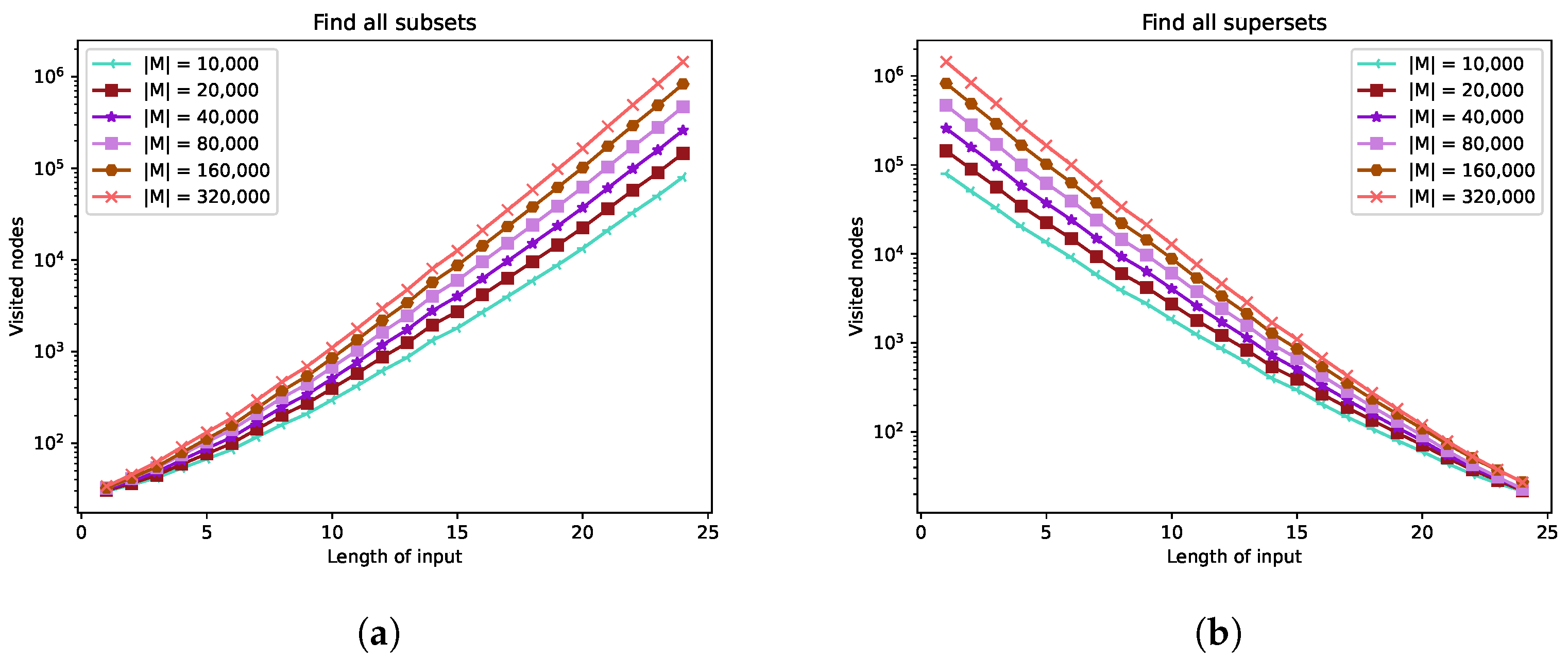
This experiment shows the performance of multiset-trie being used for storing and retrieving sets instead of multisets. We restrict multiset-trie in order to obtain a closer comparison with the set-trie data structure [24]. In this case, we set the maximal node degree n to be 2 and $\sigma$ to be 25. The mapping $\varphi$ does not have an influence in this particular experiment because the input data are generated artificially with uniform distribution. On average, the results will be the same for any $\varphi ,$ since all the multisets are equally likely to appear in $M.$ The parameter $\left|M\right|$ varies from 10,000 sets up to 320,000 sets. According to the parameters n and $\sigma ,$ the cardinality of N is $33,554,432\approx 3.36\times {10}^7.$ Thus, the calculated density of the multiset-trie with respect to $\left|M\right|$ varies from $0.3\times {10}^{-3}$ to $9.5\times {10}^{-3}.$

The performance of the functions submsetExistence and supermsetExistence increases as the density increases (see Figure 4a,b). The results are as expected because the increase in the density increases the probability of finding a sub-multiset or super-multiset in multiset-trie, which leads to a lower number of visited nodes.

The maxima are located between 175 and 375 for submsetExistence and between 175 and 350 for supermsetExistence. According to these maxima, we can deduce that at least 7–15 multisets were checked in order to find a sub-multiset or super-multiset, which is from $0.02\times {10}^{-3}$ to $1.5\times {10}^{-3}$ of the multiset-trie and from $1.9\times {10}^{-7}$ to $4.5\times {10}^{-7}$ of the complete multiset-trie.

As the density increases, the peaks shift from the center to the left or to the right, for submsetExistence and supermsetExistence, respectively. The shifts are the consequence of the uniform distribution of sets in $M.$ Since every set has the same probability of appearing in $M,$ the distribution of set sizes in M is normal. Consequently, with the increase in the density of the multiset-trie, the number of sets in M with cardinality $\frac{1}{2}\sigma$ will be larger than the number of sets with cardinality $\frac{1}{2}\sigma \pm ϵ,$ for $\frac{1}{2}\sigma >ϵ>0.$ Thus, the function submsetExistence needs to visit less nodes for test sets of size $\frac{1}{2}\sigma$ than for test sets of size $\frac{1}{2}\sigma \pm ϵ.$ The function decreases the multiplicity of some elements (in some cases, it skips them) in order to find the closest subset. Hence, the peak shifts to the left. Oppositely, the function supermsetExistence increases the multiplicity of some elements (in this case, adding new elements) in order to find the closest superset. Thus, the peak shifts to the right.

Note that despite the peak shifts, both functions submsetExistence and supermsetExistence have approximately the same worst-case performance.

The performance of the functions getAllSubmsets and getAllSupermsets decreases as the density increases (see Figure 5a,b). This happens because the number of multisets in multiset-trie increases, which means that any multiset in the data structure will have more sub- and super-multisets. The maxima for both functions vary from $8.0\times {10}^4$ to $1.5\times {10}^6$ visited nodes. We can notice that the local maxima for the functions getAllSubmsets and getAllSupermsets differ with respect to the length of input. The explanation is very simple. In order to find all sub-multisets of a small set, the function has to traverse a small part of the multiset-trie. As the size of a set increases, the part of a multiset-trie where all the sub-multisets of a given set are stored also increases. The opposite holds for the function getAllSupermsets.

Despite the fact, that for a lookup of any set/multiset, $\sigma$ nodes must be visited in multiset-trie on average, the data structure has very similar performance results in comparison to the set-trie data structure.

5.3. Experiment 2

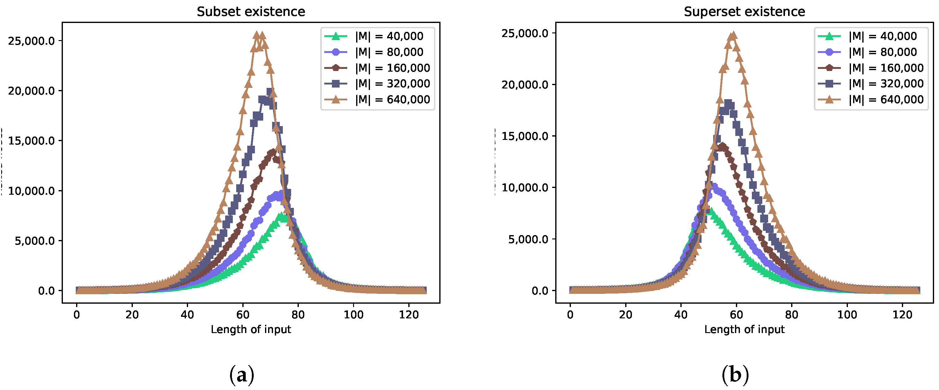
In Experiment 2, we demonstrate the performance of the unrestricted multiset-trie allowing multisets to be inserted into the data structure. We set n to be 6 and retain $\sigma =25$, as in Experiment 1. The mapping $\varphi$ does not have an influence on the results, since the input data are generated artificially with uniform distribution. The cardinality of M varies from 40,000 to 640,000 multisets. Thus, the calculated density d varies from $1.4\times {10}^{-15}$ to $2.25\times {10}^{-14}.$ The density is much smaller than in Experiment 1, because now we allow multisets to be stored in the data structure, and according to the parameters n and $\sigma$, the cardinality of N is $6^{25}=2.84\times {10}^{19}.$

As we can see from the graphs in Figure 6a,b, the performance of the functions submsetExistence and supermsetExistence becomes worse as the density increases. In this case, the number $\left|M\right|$ is slightly larger than in Experiment 1, but the density is very small. Consequently, multiset-trie becomes more sparse. Multisets in a sparse multiset-trie differ more, which leads to a larger number of visited nodes.

The maxima for both functions vary from 7500 to 25,000 visited nodes. According to these maxima, at least 300–1000 multisets were checked in order to find a sub-multiset or super-multiset, which is from $1.5\times {10}^{-3}$ to $7.5\times {10}^{-3}$ of the entire multiset-trie and from $1.1\times {10}^{-17}$ to $3.4\times {10}^{-17}$ of the complete multiset-trie. The percentage of visited multisets with respect to $\left|M\right|$ is larger than in Experiment 1. However, if one would compare the percentage of visited multisets with respect to the complete multiset-trie, then, in the case of Experiment 2, it is less by 10 orders than in Experiment 1.

The peaks are shifted from the center to the left and right for submsetExistence and supermsetExistence, respectively. Such behavior was previously observed in Experiment 1. The explanation is the same: the input data have a uniform distribution, implying that the size of multisets in M is normally distributed. Because of the normal distribution of the size of multisets, the shift in the peak occurs as the density increases.

It can also be observed that, as in the previous Experiment 1, both functions submsetExistence and supermsetExistence have similar worst-case performance.

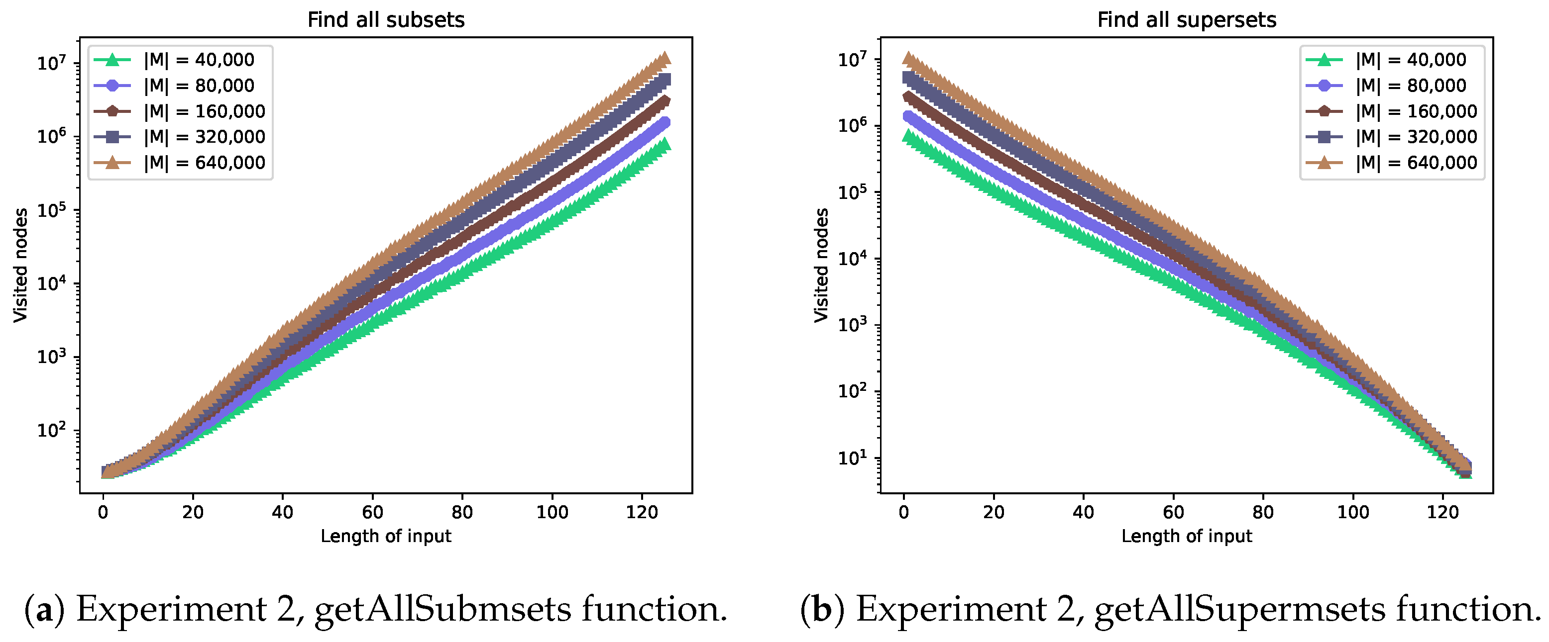
The functions getAllSubmsets and getAllSupermsets decrease their performance as the density increases (see Figure 7a,b). This happens because the number of multisets increases as the density increases. Thus, there are more nodes that have to be visited in order to retrieve all sub- or super-multisets of some multiset. The maximum for both functions varies from $0.9\times {10}^5$ to $1.5\times {10}^7$ visited nodes. As was observed in Experiment 1, the maxima occur at opposite points. For the function getAllSubmsets, it will always be at the largest size of the multiset, which is 125 in our case. Conversely, the maximum for getAllSupermsets is at the smallest size of multiset, which is 0 (an empty set).

The results of Experiment 1 show that the performance of functions submsetExistence and supermsetExistence increases as the density increases. However, we observe the opposite behavior in Experiment 2. We explain the reason for such a contradiction in the next Experiment 3.

5.4. Experiment 3

The results of Experiment 1 and Experiment 2 have shown that as the density of a multiset-trie increases, the performance of functions submsetExistence and supermsetExistence can both become better and worse. The reason for such behavior is that the dependence of the number of visited nodes on the density is not a linear function. The performance of the abovementioned functions is maximal when the multiset-trie is complete. As the multiset-trie becomes more sparse (the density is small), the multisets differ more, and the number of visited nodes increases. However, the multisets differ less when the density is high, so the number of visited nodes decreases. Since the dependence of the number of visited nodes on the density of multiset-trie is a continuous function in the interval $[0,1],$ there exists a global maximum. In other words, there exists such a value of density where the number of visited nodes is maximal.

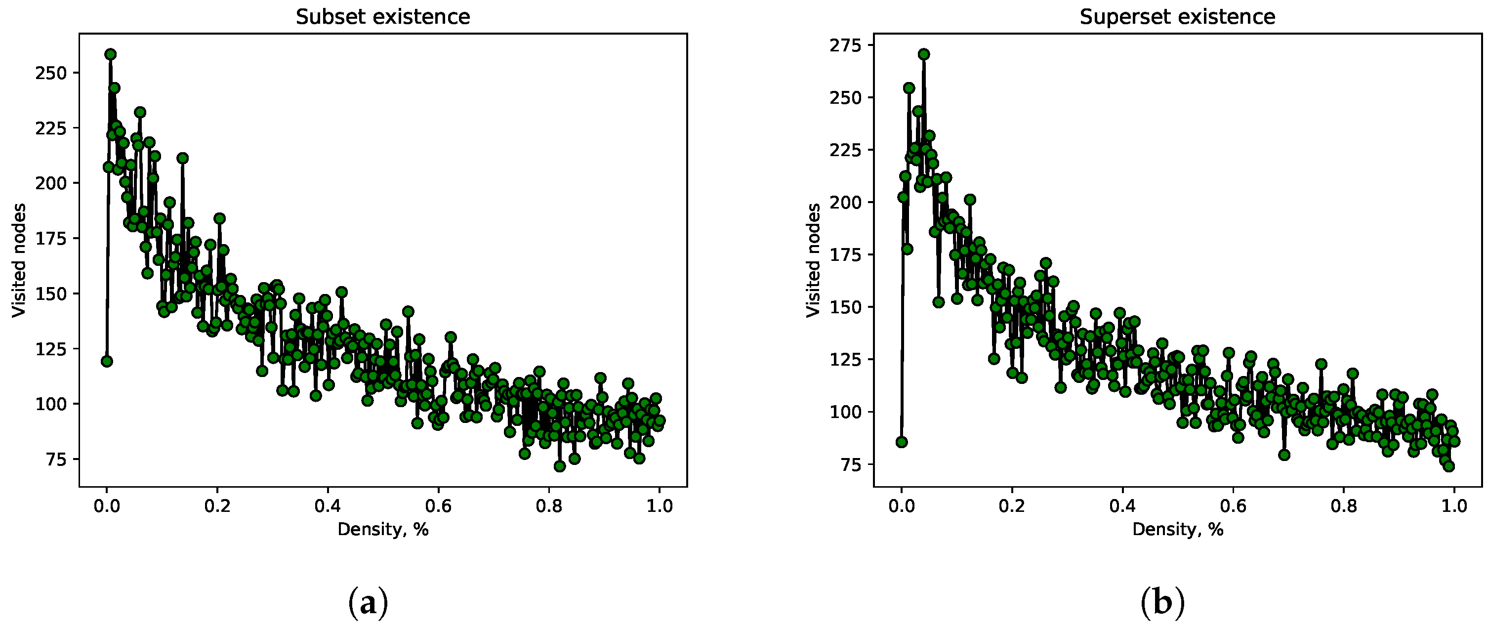
In this experiment, we empirically find the extremum of density for functions submsetExistence and supermsetExistence. The parameters $\sigma$ and n are set to 12 and 5, respectively. The density varies from $1.0\times {10}^{-6}$ to $1.0\times {10}^{-2}.$ The number of visited nodes was chosen to be maximal for each value of a particular density.

As we see in Figure 8a,b both functions submsetExistence and supermsetExistence have the maximum around $d\approx 7.0\times {10}^{-5}.$ The maximum is less than $0.3\times {10}^{-3}$ and greater than $1.4\times {10}^{-15},$ which explains the behavior of multiset-trie in Experiment 1 and Experiment 2. It is safe to say that the maximum may vary depending on parameters n and $\sigma ,$ but such a maximum always exists. Therefore, we omit the experiments with different parameters n and $\sigma .$

5.5. Experiment 4

In previous experiments, the input was generated artificially with a uniform distribution, so there was no influence of the mapping function $\varphi$ on the performance of the tested functions. This experiment shows the influence of the mapping $\varphi$ from alphabet $\Sigma$ to a set of consecutive integers. We obtain the influence by taking the real-world data as input data.

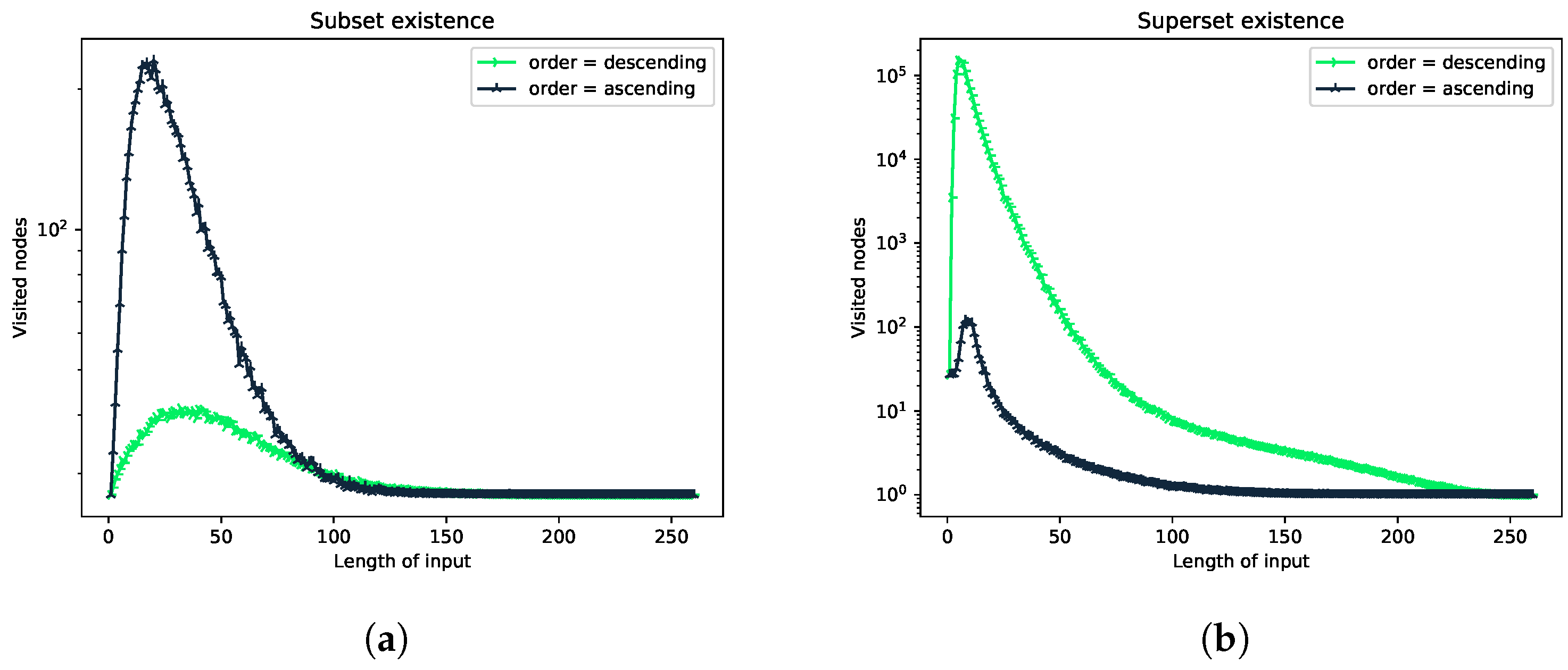
The data are taken from the English dictionary, which contains 235,883 different words. These words are mapped to multisets of integers according to the $\varphi .$ In particular, we are interested in cases where $\varphi (\Sigma )$ enumerates letters by their relative frequency in the English language. We say that $\varphi (\Sigma )$ maps letters in ascending order if the most frequent letter is mapped to number $\sigma .$ Conversely, in descending order, this letter is mapped to the number $1.$ The size of the alphabet $\sigma$ is set to the size of the English alphabet: 26. The degree of a node n is set to 10. On average, the multiplicity of letters is, of course, less than 10. We choose such a large node degree allowing the multiplicity to be up to 10 because the dictionary contains such words.

The results in Figure 9a,b are more balanced when letters are ordered by frequency in ascending order. The maxima for the functions submsetExistence and supermsetExistence are at 250 visited nodes.

According to the design of the data structure multiset-trie, we can say something about multiset only if we try to reach it, i.e., to find the complete path that corresponds to a particular multiset. This means that in order to give an answer about the existance of some multiset, one has to check the leaf level in multiset-trie.

Letters that have the least frequencies are now located at the top of multiset-trie according to the ascending order of letters by frequency. This means that the search becomes narrower because a great deal of invalid paths will be discarded at the top-most levels. Thus, multiset-trie can be traversed faster.

As may have been noticed, the functions getAllSubmsets and getAllSupermsets were not tested in this experiment. These functions are not affected by variations in the mapping $\varphi ,$ because, for any multiset, they retrieve all sub-/super-multisets. This means that the number of visited nodes will not be changed as $\varphi$ varies.

5.6. Experiment 5

In this experiment, we demonstrate the performance of the multiset-trie data structure compared to the Inverted Index based on the B-tree. Both data structures are implemented in the programming language C++, providing in this way an experimental setup for a fair comparison [27].

The Inverted Index is implemented using an idea from [23]. An inverted index structure consists of two parts: a dictionary and postings. In our case, a dictionary is implemented as an in-memory B-tree where keys are all distinct values from a domain represented by a set $\Sigma .$ The postings are represented by lists of multisets that contain a particular element from $\Sigma .$ Each list item in postings contains a cardinality of a multiset, which speeds up the containment queries.

The experiment uses the input data for the construction of the given data structure and the test data for the execution of the operations on the given data structure. The input data comprise a set of randomly generated multisets used for the construction of a data structure. The test data include the set of multisets together with the operations that are evaluated. The input and test data were generated with respect to parameters $\sigma$ and n, as presented in

Table 1. Configuration of $\sigma$ and n in benchmark.

$\mathit{\sigma }$	n
5	1
30	1
5	3
15	3
30	3
10	10

.

We tested all three types of query on all of the configurations from Table 1, resulting in 18 experiments in total, i.e., 6 experiments per query type. In each experiment, we measured the average time consumed by the data structure to process the query. The results of the exact search, sub-multiset, and super-multiset search experiments are presented in

Table 2. Exact search.

$\mathit{\sigma }$	n	Multiset-Trie ($\mathsf{\mu }{s}$)	Inverted Index ($\mathsf{\mu }{s}$)
5	1	3.45	17,782.35
30	1	4.18	24,865.93
5	3	2.20	1508.81
15	3	4.39	2146.36
30	3	10.67	3639.97
10	10	6.93	384.05

,

Table 3. Sub-multiset search.

$\mathit{\sigma }$	n	Multiset-Trie ($\mathsf{\mu }{s}$)	Inverted Index ($\mathsf{\mu }{s}$)
5	1	8.96	73,500.84
30	1	17.33	547,572.74
5	3	117.95	162,360.43
15	3	20.74	443,321.39
30	3	23.75	947,706.14
10	10	55.59	466,022.68

, and

Table 4. Super-multiset search.

$\mathit{\sigma }$	n	Multiset-Trie ($\mathsf{\mu }{s}$)	Inverted Index ($\mathsf{\mu }{s}$)
5	1	10.63	63,073.86
30	1	14.65	449,251.68
5	3	171.04	163,256.77
15	3	43.42	425,733.80
30	3	22.06	729,831.34
10	10	58.32	373,784.81

, respectively.

We can see that multiset-trie outperforms the Inverted Index in all of the experiments by up to four orders of magnitude. In an exact search, multiset-trie has to traverse only up to $\sigma +1$ nodes to obtain a query result. It can be seen from the results that with the increase in $\sigma$, the processing time for multiset-tire also increases. Multiplicity also affects the processing time; however, this happens passively. Multiplicity, or the degree of a node n, defines the shape of multisets that are stored in multiset-trie. Thus, it affects the structure and density of the multiset-trie.

As for the Inverted Index, all three operations must first fetch all postings for each particular element of a test multiset. Afterward, the intersection of postings is computed to answer the query. The operations use more processing time than a simple tree traversal, which we can see from the results. Postings are filtered on-the-fly to reduce the cost of the intersection.

Implementations of the multiset containment operations for searching sub-multisets and super-multisets are similar in the case of the inverted file. The algorithm consists of the same steps. First, the postings are fetched for each element of the test multiset. Depending on the particular operation, postings are filtered on-the-fly. Finally, the union or the intersection of the filtered set of postings is computed. Note that the processing time increases with the size of the inverted index because of the increased sizes of postings.

In the case of multiset-trie, only a traversal of the tree is required, which is much faster than the processing of postings, as we can see from the results. In the worst case, the whole tree is traversed, but the same is for an inverted file.

6. Related Work

The data structure multiset-trie is related to the data structures and indexes designed to store and manage sets and multisets. We mainly focus on the related data structures and indexes that efficiently support the set and multiset containment queries. Firstly, we summarize our previous work on the data structure for managing sets in Section 6.1. Next, we present in Section 6.2 the related work on the inverted files, i.e., the index structure that serves as a central data structure in the area of Information Retrieval (IR), but also for storing sets and multisets in database management systems. The alternative to the inverted file is the signature tree that is presented in Section 6.3. Finally, we describe the related work in the area of database management systems in Section 6.4. We review the novel index structures used for the containment queries and the proposed containment join algorithms.

6.1. Set-Trie

The multiset-trie is closely related to the set-trie data structure introduced by Savnik in [1,24]. A set-trie is a trie data structure that is adapted for the efficient storage and retrieval of sets instead of the sequences of symbols. The set-trie provides the set containment operations, such as the retrieval of the nearest subset or supersets, as well as the retrieval of all subsets and supersets from the sets of sets.

Since we are storing sets where each element of the set can appear only once, and the ordering of elements is not important, the ordering of the elements from the alphabet can be used for guiding the search in set containment operations. Each set is represented in a set-trie by a path including the increasing elements of a set represented by set-trie nodes. Since all sets from a set-trie are ordered by the increasing value of the set elements, the children of each set-trie node n can only be elements larger than the element n. For a given set s and a set-trie S, the set containment operations search solely the subtree of S that includes all the sets (paths from a root to a set-trie node) that are the possible subsets or supersets of s.

The data structure multiset-trie generalizes the set-trie by providing storage for the set of multisets. When the multiset-trie is restricted to store a set of sets, the underlying data structure becomes a simple binary tree. Moreover, all the operations of the set-trie are also supported by the multiset-trie. The generalization comes with a small penalty in performance if we compare the multiset-trie with the set-trie in the performance of the set containment operations. The downside of such a generalization is that multiset-trie no longer supports the path compression that was obtained in set-trie.

6.2. Inverted File

The inverted file [6,7,16] is the most common data structure used to represent a collection of (multi)sets. In the area of IR [8], the inverted files are used for searching documents that contain a given set of words. It is composed of two parts: a dictionary and the postings. The dictionary maps each word to a list of document identifiers together with the locations of words in documents. The dictionary is most often implemented by a variant of a search tree, such as a B+ tree. The postings are implemented as a list of positions that are stored on the disk because of the huge amount of documents usually indexed by the inverted file. Since we can have a large number of postings for one word, the postings are compressed. Furthermore, several possible optimizations exist in the representation and implementation of postings [7], such as the sorting of postings, a technique called skipping, and others.

The empirical analyses [16,23] show that the inverted file is the most efficient data structure for containment queries among the data structures: the sequential signature file, the signature tree, the extendible signature hashing, and the inverted file.

6.3. Signature Trees

A dynamically balanced signature tree [20,28], or S-tree, is an alternative data structure for the representation of multisets. An S-tree stores objects on the basis of their attributes represented in the form of signatures. A signature of an object is formed by the discretization of object attributes. Each attribute is discretized by mapping the attribute values to a sequence of bits. The bit sequences are the abstractions of the values of object attributes. They are glued together to form the signature of an object. The mappings from attribute values to sequences of bits are defined in such a way that allows superimposing a set of signatures by a single signature. Such a signature is often formed by using the operation OR. This property of signatures provides the means for the construction of the hierarchy of signatures that is utilized for efficient search. The multisets can be effectively represented using signatures, and the superposition operation can be implemented by the operation OR. The use of the signature tree for the containment operations was studied by Tousidou et al. [21]. They show that an S-tree that uses linear hash partitioning can be used to implement the containment operations efficiently.

6.4. Multisets in Relational Databases

The index structures for the efficient implementation of the (multi)set containment queries were studied in the framework of the relational DBMS as well as the object-relational DBMS, where we can use multivalued attributes, including sets, multisets (bags), and lists. Zhang et al. [29] compared the performance of the containment queries implemented in a standard relational DBMS (RDBMS) to an information retrieval engine. The results show that, in general, the IR engine performs better than an RDBMS on containment queries. The significant causes that differentiate the performance of the IR and RDBMS implementations are the join algorithms employed and the hardware cache utilization. The differences in join algorithms and the cache access method that makes IR queries faster were identified precisely. First, the multi-predicate merge join of the IR engine is different from the standard merge join, and the index nested-loop join algorithms. Second, the study of the utilization of cache in the multi-predicate merge join, standard merge join, and index-nested loop joins has been done, identifying more precisely the differences in the algorithms. They have presented that with some modifications, an RDBMS could perform this class of queries more efficiently.

The joins in an object-relational DBMS can be defined by means of the containment operations. A number of containment join methods have been proposed [30,31,32,33]. Ramasamy et al. propose the use of the partitioning set join that relies on the representation of sets by using signatures [30]. The signature-based representation allows the efficient implementation of the set comparison operations. The partitioning set join was further improved by Melnik et al. [31] to handle large sets and to speed up the partitioning phase of the algorithm. Further, Jampani et al. introduced the PRETTI join algorithm, which combines an inverted file with a prefix tree for the efficient implementation of the containment joins. The algorithm for $R\bowtie T$ recursively computes record identifiers from T while traversing a prefix tree storing the sets from R. The algorithm uses a single intersection of two lists to enumerate the matching pairs of rid-s. The PRETTI algorithm was improved by Luo at al. [33] by replacing the prefix tree with the Patricia tree.

7. Conclusions and Future Work

One of the conclusions of studying the multiset-trie both theoretically and empirically is that our data structure is input-sensitive. Input sensitivity implies non-consistent performance on different input data. However, our argument that the performance can be optimized by pre-processing the input data is confirmed in Experiment 4. Pre-processing determines the optimal encoding for input data and ensures the best performance of the multiset-trie on particular input data. For example, in the case of storing words in the multiset-trie, the search queries can always be optimized based on the frequencies of letters in a specific language. We also see from Experiments 1 and 2 that the dependence of the multiset-trie’s performance on the density is not a linear function. However, the function is continuous, and the point of inflection is unique on the whole domain, as shown in Experiment 3. This allows us to predict whether multiset-trie can be used for some particular application, offering high performance.

The mathematical analysis section provides a non-trivial insight regarding the behavior of the multiset-trie data structure when used in randomized data. It is estimated that the space complexity of multiset-trie is of order $O\left(\right|M\left|\right)$, which is the minimal possible space required by any data structure for the storage of $\left|M\right|$ objects. As for the running time complexity of algorithms, the basic tree functions such as insert, search, and delete all have constant complexity once the multiset-trie is defined. The “getAll” multiset containment functions have the worst-case running time complexity of $O\left(\right|\mathcal{M}\left|\right),$ where $\left|\mathcal{M}\right|$ is the cardinality of the multiset-trie data structure. The “existence” multiset containment functions have the worst-case running time complexity of $O\left(\right|\mathcal{M}|-|M\left|\right),$ where $\left|\mathcal{M}\right|$ is the cardinality of the multiset-trie and $\left|M\right|$ is the number of inserted multisets (nodes on leaf level).

The implementation of the multiset-trie is not optimized. For example, the main reason for the space inefficiency is in implementing the links from a node to its children. Our implementation uses an array data structure to link a node to its children, where each element of an array, indexed by the multiplicity of the element of the next level, includes a link to a subtree. A custom-implemented small and extendable hash table would significantly decrease the amount of space needed to represent a multiset-trie.

Further steps in our research will be to extend the functionality of the multiset-trie. We are interested in more flexible multiset containment queries where additional conditions constrain the sub- and super-multisets. For example, the multiplicity of an element in a multiset can be bounded in operations getAllSubmsets and getAllSupermsets. Furthermore, the similarity search on multisets can be implemented by modifying the algorithms for searching the sub- and super-multisets. The second line of research is to investigate the multiset-trie as a database index data structure. A disk-based index data structure allows for storing and managing a huge amount of multisets. The mapping from a multiset-trie, i.e., a n-ary search tree, to a block-based index can be easily defined because of the regularity of multiset-trie. It will be interesting to compare the multiset-trie with other existing disk-based index data structures.

References

- Savnik, I.; Akulich, M.; Krnc, M.; Škrekovski, R. Data structure set-trie for storing and querying sets: Theoretical and empirical analysis. PLoS ONE 2021, 2, e0245122. [Google Scholar] [CrossRef] [PubMed]
- Bouros, P.; Mamoulis, N.; Ge, S.; Terrovitis, M. Set containment join revisited. Knowl. Inf. Syst. 2016, 49, 375–402. [Google Scholar] [CrossRef] [Green Version]
- Gripon, V.; Rabbat, M.; Skachek, V.; Gross, W.J. Compressing multisets using tries. In Proceedings of the 2012 IEEE Information Theory Workshop, Lausanne, Switzerland, 3–7 September 2012; pp. 642–646. [Google Scholar]
- Ross, K.A.; Stoyanovich, J. Symmetric relations and cardinality-bounded multisets in database systems. In Proceedings of the Thirtieth International Conference on Very Large Data Bases, Volume 30, VLDB Endowment, Toronto, ON, Canada, 29 August–3 September 2004; pp. 912–923. [Google Scholar]
- Steinruecken, C. Compressing sets and multisets of sequences. IEEE Trans. Inf. Theory 2015, 61, 1485–1490. [Google Scholar] [CrossRef]
- Zobel, J.; Moffat, A.; Sacks-Davis, R. An efficient indexing technique for full-text database systems. In Proceedings of the 18th Conference on Very Large Data Bases, Morgan Kaufmann, Vancouver, BC, Canada, 23–27 August 1992; p. 352. [Google Scholar]
- Zobel, J.; Moffat, A. Inverted files for text search engines. ACM Comput. Surv. (CSUR) 2006, 38, 6. [Google Scholar] [CrossRef]
- Manning, C.D.; Raghavan, P.; Schütze, H. Introduction to Information Retrieval; Cambridge University Press: Cambridge, UK, 2008; Volume 1. [Google Scholar]
- Mannila, H.; Toivonen, H. Levelwise Search and Borders of Theories in Knowledge Discovery. Data Min. Knowl. Discov. 1997, 1, 241–258. [Google Scholar] [CrossRef]
- Flach, P.A.; Savnik, I. Database Dependency Discovery: A Machine Learning Approach. AI Commun. 1999, 12, 139–160. [Google Scholar]
- Forgy, C. Rete: A Fast Algorithm for the Many Pattern/Many Object Pattern Match Problem. Artif. Intell. 1982, 19, 17–37. [Google Scholar] [CrossRef]
- Bayardo, R.J.; Ma, Y.; Srikant, R. Scaling up All Pairs Similarity Search. In Proceedings of the WWW’07: 16th International World Wide Web Conference, ACM, Banff, AB, Canada, 8–12 May 2007; pp. 131–140. [Google Scholar]
- Xiao, C.; Wang, W.; Lin, X.; Yu, J.X.; Wang, G. Efficient Similarity Joins for Near-Duplicate Detection. ACM Trans. Database Syst. 2011, 36, 15. [Google Scholar] [CrossRef]
- Wang, X.; Qin, L.; Lin, X.; Zhang, Y.; Chang, L. Leveraging set relations in exact set similarity join. Proc. VLDB Endow. 2017, 10, 925–936. [Google Scholar] [CrossRef] [Green Version]
- Cormen, T.H.; Leiserson, C.; Rivest, R.L.; Stein, C. Introduction to Algorithms, 2nd ed.; The MIT Press: Cambridge, MA, USA, 2001. [Google Scholar]
- Zobel, J.; Moffat, A.; Ramamohanarao, K. Inverted files versus signature files for text indexing. ACM Trans. Database Syst. (TODS) 1998, 23, 453–490. [Google Scholar] [CrossRef]
- Broder, A.Z.; Eiron, N.; Fontoura, M.; Herscovici, M.; Lempel, R.; McPherson, J.; Qi, R.; Shekita, E. Indexing shared content in information retrieval systems. In Proceedings of the International Conference on Extending Database Technology, Edinburgh, UK, 29 March 2006; Springer: Berlin/Heidelberg, Germany, 2006; pp. 313–330. [Google Scholar]
- Terrovitis, M.; Passas, S.; Vassiliadis, P.; Sellis, T. A Combination of Trie-trees and Inverted Files for the Indexing of Set-valued Attributes. In Proceedings of the 15th ACM International Conference on Information and Knowledge Management, Arlington, VA, USA, 6–11 November 2006; ACM: New York, NY, USA, 2006; pp. 728–737. [Google Scholar]
- Terrovitis, M.; Bouros, P.; Vassiliadis, P.; Sellis, T.; Mamoulis, N. Efficient Answering of Set Containment Queries for Skewed Item Distributions. In Proceedings of the 14th International Conference on Extending Database Technology, Uppsala, Sweden, 21 March 2011; ACM: New York, NY, USA, 2011; pp. 225–236. [Google Scholar]
- Deppisch, U. S-tree: A Dynamic Balanced Signature Index for Office Retrieval. In Proceedings of the 9th Annual International ACM SIGIR Conference on Research and Development in Information Retrieval, Pisa, Italy, 1 September 1986; ACM: New York, NY, USA, 1986; pp. 77–87. [Google Scholar]
- Tousidou, E.; Bozanis, P.; Manolopoulos, Y. Signature-based Structures for Objects with Set-valued Attributes. Inf. Syst. 2002, 27, 93–121. [Google Scholar] [CrossRef] [Green Version]
- Chen, Y.; Shi, Y. Signature Files and Signature File Construction. In Encyclopedia of Database Technologies and Applications; IGI Global: Hershey, PA, USA, 2005. [Google Scholar] [CrossRef]
- Helmer, S.; Moerkotte, G. A performance study of four index structures for set-valued attributes of low cardinality. VLDB J. 2003, 12, 244–261. [Google Scholar] [CrossRef]
- Savnik, I. Index data structure for fast subset and superset queries. In Proceedings of the International Conference on Availability, Reliability, and Security, Vienna, Austria, 23–26 August 2022; Springer: Berlin/Heidelberg, Germany, 2013; pp. 134–148. [Google Scholar]
- Sedgewick, R.; Wayne, K. Algorithms, 4th ed.; Addison-Wesley Professional: Boston, MA, USA, 2011. [Google Scholar]
- Gardiner, C.W. Stochastic Methods; Springer: Berlin/Heidelberg, Germany; New York, NY, USA; Tokyo, Japan, 1985. [Google Scholar]
- Akulich, M. Mstrie Repository. 2019. Available online: https://github.com/nick-ak96/mstrie (accessed on 10 March 2023).
- Pfaltz, J.L.; Berman, W.J.; Cagley, E.M. Partial-match Retrieval Using Indexed Descriptor Files. Commun. ACM 1980, 23, 522–528. [Google Scholar] [CrossRef]
- Zhang, C.; Naughton, J.; DeWitt, D.; Luo, Q.; Luo, Q.; Lohman, G. On Supporting Containment Queries in Relational Database Management Systems. In Proceedings of the SIGMOD, Portland, OR, USA, 14–19 June 2020; ACM: New York, NY, USA, 2001; pp. 425–436. [Google Scholar] [CrossRef]
- Ramasamy, K.; Patel, J.M.; Naughton, J.F.; Kaushik, R. Set containment joins: The good, the bad and the ugly. In Proceedings of the 26th VLDB Conference, Morgan Kaufmann, Cairo, Egypt, 10–14 September 2000. [Google Scholar]
- Melnik, S.; Garcia-Molina, H. Adaptive Algorithms for Set Containment Joins. ACM Trans. Database Syst. 2003, 28, 56–99. [Google Scholar] [CrossRef]
- Jampani, R.; Pudi, V. Using Prefix-Trees for Efficiently Computing Set Joins. In Proceedings of the Database Systems for Advanced Applications, 10th International Conference, DASFAA 2005, Beijing, China, 17–20 April 2005; pp. 761–772. [Google Scholar] [CrossRef]
- Luo, Y.; Fletcher, G.H.L.; Hidders, J.; Bra, P.D. Efficient and scalable trie-based algorithms for computing set containment relations. In Proceedings of the 31st IEEE International Conference on Data Engineering, ICDE 2015, Seoul, Republic of Korea, 13–17 April 2015; pp. 303–314. [Google Scholar] [CrossRef]
Figure 1.
Example of multiset-trie structure containing multisets . The Null children are omitted.
Figure 2.
Size of a tree () compared to the number of stored sets (), as the probability parameter p increases. Parameters and n are 26 and respectively. The additional overhead space that our data structure uses does not increase as the tree is becoming more and more dense.
Figure 3.
The ratio of “data overhead” derived from Figure 2, as the density p of our data structure increases. Unless we are in a very sparse setting, the trade-off in terms of space is small.
Figure 4.
Existence functions of Experiment 1. (a) submsetExistence; (b) supermsetExistence.
Figure 5.
Exhaustive functions of Experiment 1. (a) getAllSubmsets; (b) getAllSupermsets.
Figure 6.
Existence functions in Experiment 2. (a) submsetExistence; (b) supermsetExistence.
Figure 7.
Exhaustive functions in Experiment 2.
Figure 8.
Existence functions in Experiment 3. (a) submsetExistence; (b) supermsetExistence.
Figure 9.
Existence functions in Experiment 4. (a) submsetExistence; (b) supermsetExistence.