1. Introduction
Compared with 2D data, 3D data contains rich spatial information and target details, providing the possibility to achieve more detailed computer vision tasks. At the same time, with the development of 3D vision technology, the cost of acquiring and processing 3D data is getting lower and lower, thus giving rise to emerging application areas such as autonomous driving [
1,
2,
3], augmented reality [
4,
5], and robotics. In recent years, how to process 3D data with the help of deep learning methods [
6,
7,
8], which are more mature in the field of 2D image research [
9,
10,
11,
12,
13,
14], has received a great deal of attention from scholars. However, unlike a 2D image where pixels are uniformly distributed on a 2D grid, a 3D grid is a collection of connected relationships between a series of points and edges in 3D space. This means that the 3D grid model does not have a regular 3D spatial representation, while the input of data is disordered. The structural differences between 2D images and 3D grid models make it impossible to directly apply the more mature neural network design in the field of 2D image research to 3D mesh models.
To overcome the problem of irregularity and disorder in 3D grid models, some studies have pioneered attempts by designing the input format of 3D grid model data and 3D convolution and 3D pooling methods [
15,
16,
17,
18]. Feng et al. and Hanocka et al. [
16,
17] used grid or grid edge as the basic unit to define the standard input format of 3D grid models and, based on the input features, for 3D grid models design convolutional classification networks based on the input features. However, although the convolution and pooling process can weigh the combination of lower-level features to form higher-level features, the spatial information and dependencies of the lower-level features in the higher-level features are lost [
19]. Especially in 3D space, the 3D model is richer in location structure information and the local–local interrelationships are closer.
To preserve inter-feature dependencies, inspired by the self-attentive mechanisms that have been successful in the natural language domain and in the 2D image domain, work such as point cloud transformer (PCT) [
20], point transformer (PT) [
21], and transformer (METRO) [
22] in a 3D point cloud model analysis using transformer architecture. However, these methods applied to the 3D domain encode the input in a way that does not design a self-attentive mechanism based on the local features of the 3D model and are not as interpretable as tokens in NLP. At the same time, such transformer networks, which are stripped from the original convolutional architecture, tend to retain the multi-layered characteristics of convolutional networks, which often implies a huge computational overhead when combined with the self-attentive mechanism with
O(
n2) time complexity in a transformer [
23].
Based on the characteristics of convolutional networks and transformer networks, this paper proposes a self-attentive convolutional network MixFormer for 3D mesh models. The shape features of 3D mesh models are extracted as the semantic information input to the transformer module through the front 3D mesh convolutional module. To ensure that the 3D mesh convolution module can effectively extract the feature information of the 3D mesh model, a 3D convolution kernel is defined in this paper. The introduction of the 3D mesh transformer module enables the network to learn the global association among the 3D mesh shape features, which makes up for the deficiency of the convolution operation in learning long-distance features. And by introducing a vector-type self-noticing mechanism in the transformer network, the spatial information of the 3D grid model is introduced, which makes the transformer module better applicable to the 3D grid model.
In this paper, we conducted classification experiments on SHREC15 and Manifold40 datasets, and segmentation experiments on SCAPE, FAUST, and MIT datasets, and demonstrated the effectiveness of each module on 3D feature learning by ablation experiments. The experiments show that MixFormer can achieve good learning results without stacking multiple layers and with less computational overhead by learning local feature information through the front 3D grid convolution module and establishing dependencies between features by the 3D grid transformer.
In summary, the main contributions of this paper are as follows.
- (1)
A 3D convolutional kernel applicable to 3D mesh models is designed to enable the network to extract feature information on 3D grid models with irregularities and disorder.
- (2)
The vector-based transformer module is designed to better learn the dependencies between features through a vector-based self-attentive mechanism and a learnable position encoding.
- (3)
The shape features extracted by the convolutional network are processed by using the self-attentive mechanism with a pyramidal structure, so that the network can fully establish global feature dependencies while extracting feature information more accurately.
3. MixFormer
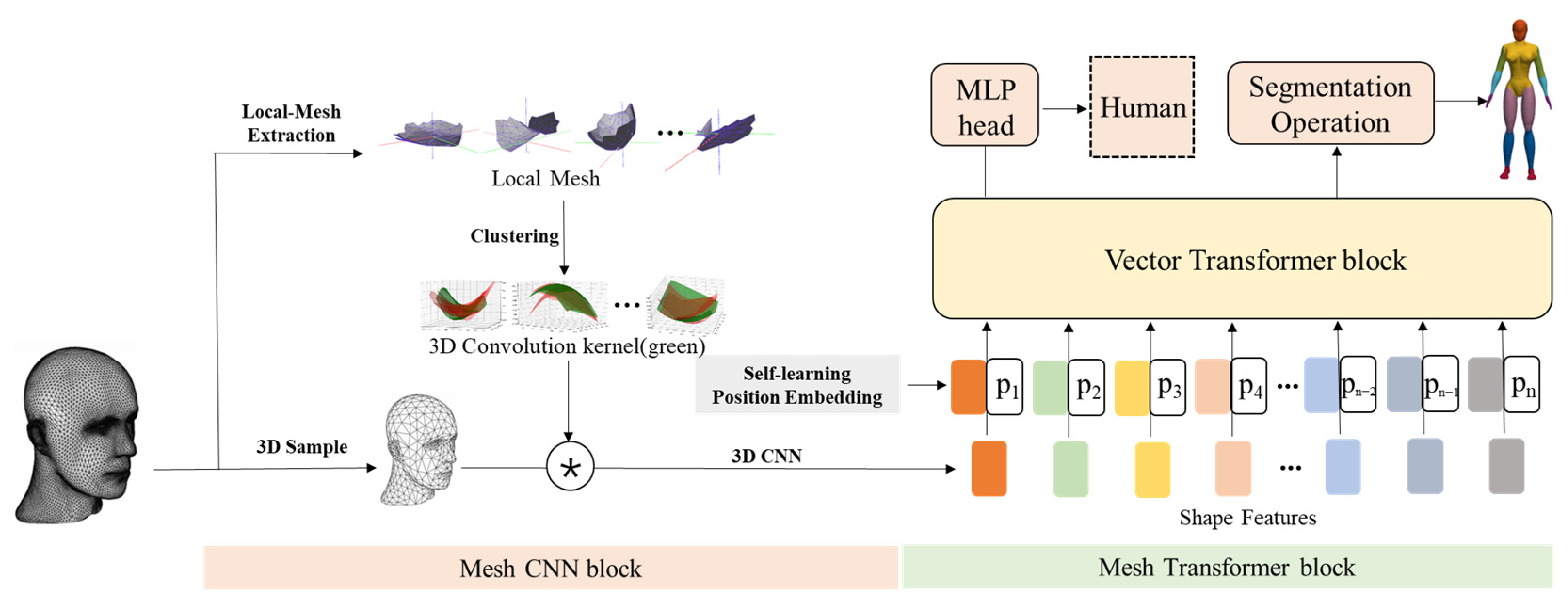
In this paper, we propose a vector self-attention convolutional network, MixFormer, applied to 3D mesh models from the perspective of local feature learning to establish global feature dependencies. The specific network model design is shown in
Figure 1, which can be divided into the following two major blocks.
3D mesh convolution block: For the input 3D mesh data, the 3D mesh convolution block defines the local surface by polynomial expression, and acquires the 3D convolution kernel by aggregating the local surface features through clustering operation. Then the data is reduced by 3D sampling to get the shape feature representation of 3D mesh model data.
3D mesh transformer block: for the shape feature representation of the 3D mesh model data obtained after processing by the convolution block, the spatial feature information of the 3D mesh model is introduced through the learnable position encoding, and the global dependency of its high-level semantic features is established using the vector self-attention, so as to realize the downstream tasks such as classification and semantic segmentation of the 3D mesh models.
Compared with previous methods, this method has the following advantages: (1) A learnable 3D convolutional kernel template is introduced to cope with the problem that traditional convolutional operations are difficult to apply to 3D mesh models. (2) The transformer block, which is suitable for establishing long-distance dependencies, is introduced to learn the association between global features and make up for the deficiency of the convolution block in learning long-distance features. (3) The combination of the convolution block and the transformer block, which learns the shape features in the 3D mesh model through the pre-convolution operation and then establishes the association between the features through the transformer block, makes MixFormer achieve good classification and segmentation results without building a multi-level network architecture. Compared with other network models applied to 3D mesh models, the number of parameters and computational effort is significantly reduced.
3.1. 3D Mesh Convolution Block
To perform convolutional operations on surface features of complex 3D mesh models, a polynomial convolutional kernel is designed in this paper. The method is described as follows.
Taking the vertices of the 3D mesh model as the center of the window, we first perform a breadth-first search on each vertex to obtain its K-neighborhood, and call the 3D mesh surface formed by the vertices and interconnected edges contained in its K-neighborhood a local surface window. For the local surface window, we define the polynomial representation equation of the local surface and fit the surface by weight learning to obtain the polynomial expression of the local surface. The obtained polynomials for local surfaces are then clustered to extract the 25 surface shapes commonly found in the model as the base convolution kernels. The similarity of each local surface to the basic surface convolution kernel is obtained by convolving each local surface using the basic surface convolution kernel. This is used as the local surface feature of the vertex neighborhood.
3.1.1. Mesh Local Surface Representation
First of all, since the same model in the 3D model undergoes translation or rotation, its polynomial expression parameters are changed accordingly. In order to eliminate the effect of translation and rotation on the features, the grid window needs to be orthogonalized so that its window center is the origin of the new coordinate system (translation) and its normal vector is the z-axis of the new coordinate system (rotation).
Second, for each vertex’s K-neighborhood, we have the following definition.
Here denotes the set of vertices contained in the K-neighborhood of vertex , is the set of vertices contained in the window with vertex as the window center, and is the set of edges contained in the window with vertex as the window center.
Since the local window contains only a small amount of 3D surface mesh when the local window is designed small, the ability to aggregate its neighborhood information is limited. Moreover, when the window is designed larger, the window shape becomes complex, and the original 3D coordinates of the vertices alone are not sufficient to describe the mesh features. Therefore, geodesic distances are introduced in related works. However, the calculation of geodesic distance often requires a lot of computational resources, so block distance d is chosen as the approximation of geodesic distance.
Therefore, the fitting function of the local window is shown in Equation (3).
Let the fitting function of the local window surface equal to 0, train the learnable parameters therein, and fit the local surface polynomial. The function obtained after fitting is the approximate representation of the local window.
In the training process, the loss function is the mean loss:
In order to obtain the basis surfaces in the model as the base convolution kernel, the obtained local window expression features need to be clustered. In this paper, it is divided into 25 types of basis surfaces. The feature representation of the base surface obtained by clustering is the base convolution kernel. Finally, we use the base convolution kernel to convolve each positive-definite local surface to obtain the similarity between the local surface and the base surface as its shape features.
3.1.2. Similarity Measure
In order to perform the clustering operation on the local window, the similarity definition of the local surface polynomials is needed to evaluate the clustering effect. To define the similarity between local surfaces, in this paper, the average distance between surfaces is used as a measure of the similarity between surfaces. For this purpose, combined with Equation (3), we have the following equation:
where the surface polynomials
and
corresponding to the local surface
and the target surface
(the center of clustering), respectively.
denotes the distance between the points of the local surface
and the target surface
. Since Equation (5) only represents the one-way distance, to reduce loss, we define a two-way difference metric based on Equation (5).
For each local spatial surface of the 3D mesh model, the polynomial representation function is
. We assume that the local space surfaces in the 3D mesh model obey a Gaussian distribution on the data with variance
σ and mean
μ. Then, for any local space surface
, the probability that the surface belongs to the target surface is Equation (7).
3.1.3. Definition of 3D Convolution Operations
In the convolution operation of 2D images, the 2D convolution kernel convolves the local image, the essence of which can be understood as computing the similarity between the 2D convolution kernel and the local image. In
Section 3.1.2, we define the similarity function
, which is used to perform the clustering operation on the local surface windows to obtain the standard surface windows (clustering centers). The standard surface window obtained by the clustering operation can be used as a 3D convolution kernel for the 3D convolution operation. The 3D convolution operation is the process of calculating the 3D convolution kernel and the local surface window, so the similarity measure can still be used in Equation (7).
To make the similarity function
closer to the common convolution operation, taking the logarithm of the full probability equation yields.
This formula can be converted into a convolution formula:
represents the feature vector
and
represents the feature at vertex
. For example 0, 1 can represent the presence or absence of vertex
on a local surface, where
represents the weight vector
, and b represents the bias corresponding to the feature vector.
3.1.4. Three-Dimensional Sampling
After the convolution operation by the polynomial convolution kernel, each vertex aggregates the local surface features of its neighborhood. However, this introduces a new problem, as each vertex contains the local surface features of its neighborhood, so there is a large amount of data redundancy. To reduce the amount of data in the network, 3D sampling can be performed based on the vertices.
Unlike the 3D point cloud models, the 3D mesh models represent the contour features of the model by the combination of vertices and triangulated facets, and the vertices and triangulated facets are also not uniformly distributed on the model, showing a partly dense and partly sparse feature. Therefore, if the vertices are to be sampled, the farthest sampling method, which is commonly used in point cloud models to cover all points in space as uniformly as possible, is not very suitable for 3D mesh models. To solve this problem, we found that Poisson disk sampling can achieve uniform sampling according to the model contour.
The algorithm for Poisson disk sampling is shown in Algorithm 1.
| Algorithm 1: Poisson disk sampling |
Input: Input vector , desired number of samples
Output: Output vector Build a kd tree for samples for each sample to store the weights Si ← pull the top sample from heap For each sample around Remove from Update the heap position of
|
3.2. 3D Mesh Transformer Block
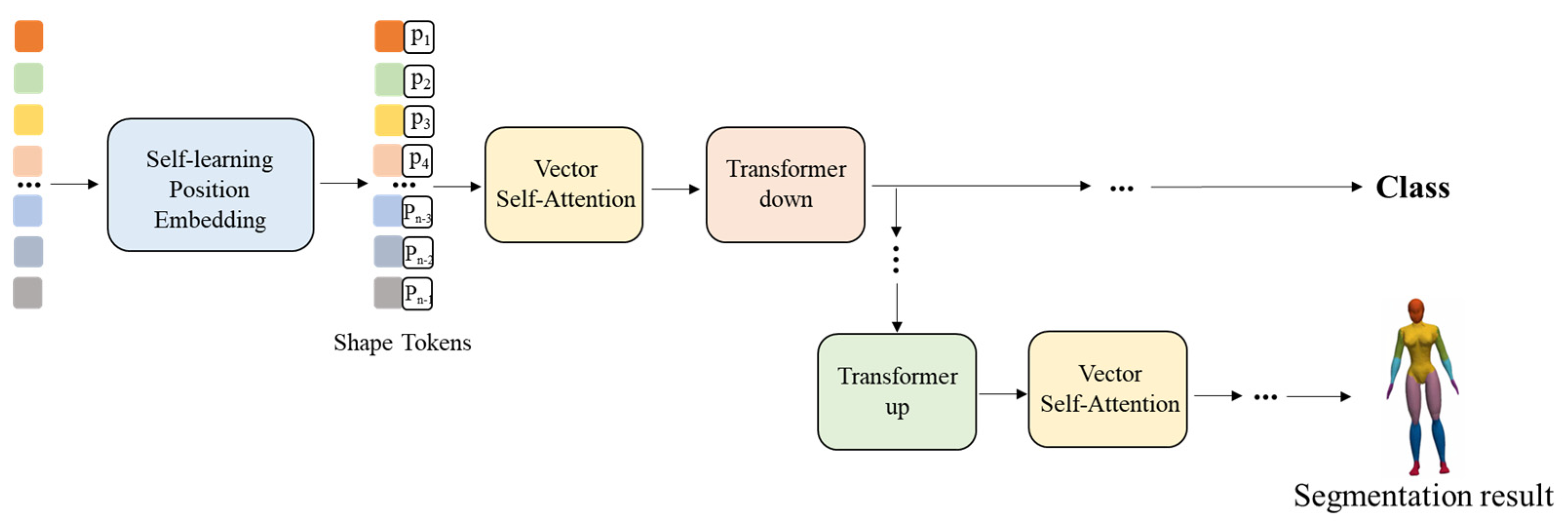
Through the 3D convolution operation, we extract the local shape features of the 3D mesh model. In order to establish the dependencies between the features, the local shape features of the 3D mesh model need to be input into the 3D mesh transformer block. The core structure of the 3D mesh transformer block is shown in
Figure 2.
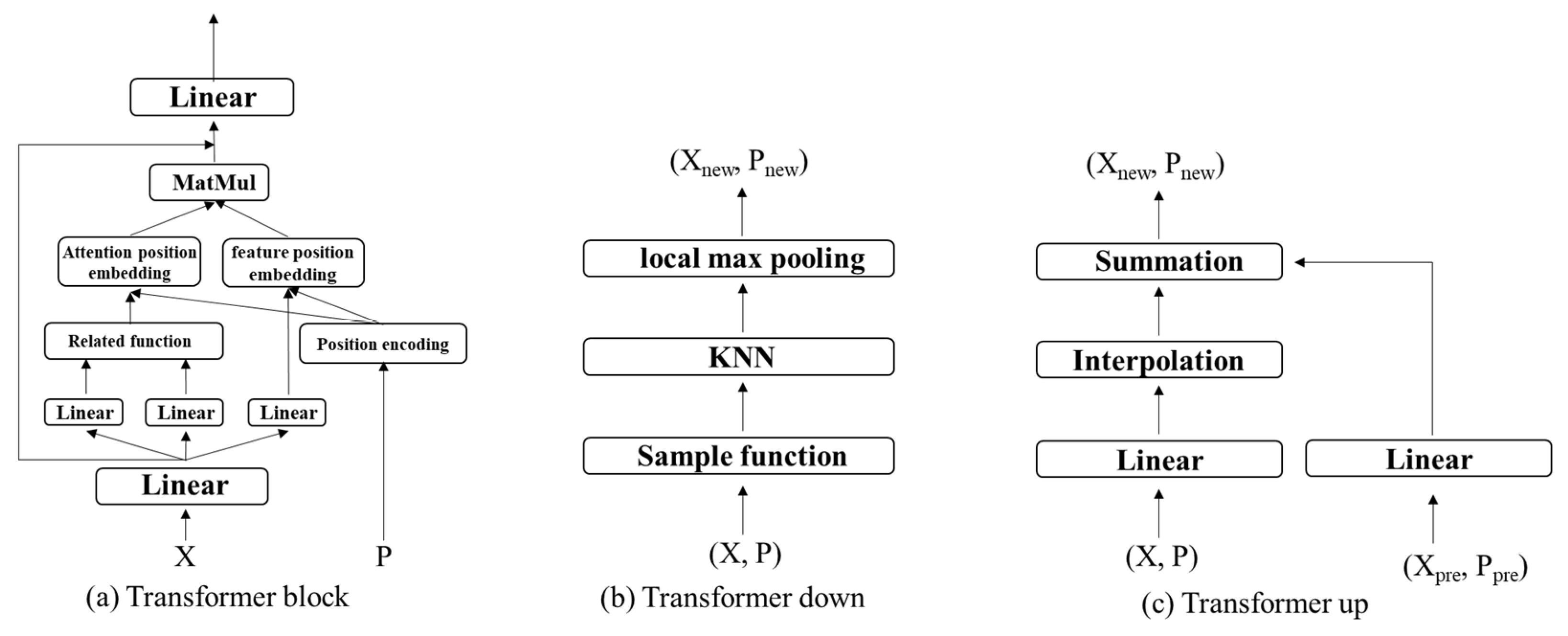
Considering the disorder of data in the 3D mesh model, i.e., the model features of the vertices in the 3D mesh are independent of the input order, an MLP network with shared weights is introduced in the first layer of the network to eliminate the effect of input order and extract the 3D mesh model features, feature mapping is performed for local shape features, and then the 3D mesh is mapped through multiple transformer layer and down layers to The global features of the model are then learned through multiple transformer layers and down layers. Finally, the features of the model are aggregated by a global maximum pooling operation and the model type is predicted by an MLP layer. For semantic segmentation operation, the transformer up layer is introduced to restore features to predict the semantic labels of mesh. The internal implementation of the transformer layer, down layer, and up layer is shown in
Figure 3.
3.2.1. Vector Self-Attention
The core of the model is the transformer layer containing residual blocks. vector self-attentiveness enables the exchange between local features and the acquisition of associations between global features. By linear mapping, the dimensionality of the data computed by the vector-based self-attention can be reduced.
The input of the traditional transformer’s self-attention contains three matrices,
,
and
.
,
represent query, key, and value.
,
is like a key–value relationship, which is a one-to-one correspondence.
Self-attentions can be divided into two categories: scalar self-attentions and vector self-attentions.
The scalar self-attention can be expressed as Equation (13).
Corresponding to each input feature
,
is the output feature. ψ is a normalization function, such as softmax. pos is a position encoding function.
q,
k, and
v represent the query, key, and value generated by the corresponding
. It can be expressed as Equation (14).
, , and are affine transformations, such as linear mappings or multilayer perceptrons.
In vector self-attentions, the representation of the self-attentive functions differs, like in Equation (15).
is the set of vertices representing the vertices adjacent to , and φ is a correlation function, e.g., +, −, ×, or ⊙. α is a mapping function that maps a self-attentive vector to a self-attentive feature, e.g., MLP.
For the 3D mesh model, the 3D mesh transformer layer used in this paper is based on the vector transformer design. The obtained self-attention function is as follows.
is the set representing the vertices adjacent to (in this experiment it is the nearest neighbor k vertices), and the local self-attention mechanism is applied in the local neighborhood around each vertex. The correlation function φ is chosen as the Hadamard product, and the mapping α function is an MLP with two linear layers and a Relu layer.
3.2.2. Learnable Position Encoding
In the self-attention, positional encoding can mark the relative position relationship between elements and introduce more spatial information. Therefore, positional encoding is often introduced to enhance the model effect in natural language processing or 2D image processing. In the 3D model, its original 3D coordinate information can reflect the position relationship between elements, in order to eliminate the influence of the coordinate system and coordinate scale on the results. We introduce a learnable position encoding method.
and
denote the 3D coordinates corresponding to the vertices
and
of the 3D mesh model. β is an MLP with two linear layers and a Relu layer.
After processing by the transformer layer, new semantic features are obtained after performing local feature fusion. To reduce the number of parameters, a down layer is introduced to sample tokens. First, the input is sampled, and for processing convenience, the sampling function here is the farthest point sampling. Since some feature information is lost after sampling, the KNN method is introduced. The sampled tokens that aggregate the feature information of their K-neighborhoods are obtained by an MLP layer consisting of normalization and Relu and a K-neighborhood local maximum pooling layer.
3.2.3. Transformer down Layer
To extract the low-level features into high-level features and reduce the feature dimension, we design the transformer down layer. The transformer down layer is shown in
Figure 3b. Where X represents the input feature vector and P represents the input vertex set. X
new represents the output feature vector and P
new represents the output feature vector. First, by sampling, we select a well-distributed subset of vertices P
new, P
new ∈ P. To pool the feature vector X associated with P onto the feature vector X
new associated with P
new, we use KNN for P and then max-pool each point in P from the K neighboring points in P.
3.2.4. Transformer up Layer
For the semantic segmentation task, we combine the main modules of MixFormer with the U-net network. To decode the feature information extracted by the network, we designed the transformer up layer to map features from the set of downsampled input points P to its superset P
new. The transformer up layer is shown in
Figure 3c. For this purpose, each input point feature is processed by a linear layer, followed by batch normalization and Relu, and then the features are mapped to a higher resolution point set P
new by trilinear interpolation. Finally, the interpolated features from the previous decoder level are provided with the corresponding encoder-level feature summaries by a jump connection.
3.3. Time Complexity Analysis
At the end of this chapter, we will discuss the time complexity of the methods in this paper.
In the mesh CNN block, we use Equation (7) to perform the similarity measure between the 3D convolution kernel and the local surfaces, which is calculated only with respect to the number of points in the local surfaces, and the number of points in the local surfaces is a custom constant K, so the similarity calculation time is a constant . To obtain a specified number of standard surfaces as 3D convolution kernels by clustering, all local surfaces need to be traversed to calculate similarity. The time complexity is . In order to perform 3D convolution operation on a 3D mesh model using 3D convolution kernels, each convolution kernel needs to calculate similarity with all local surfaces, so the time complexity of convolution operation is . In summary, without considering the operations of the downsampling and local surface division, the time complexity of the 3D convolution module is , where I, k, and t can be regarded as constants, so the time complexity can be simplified to .
In the mesh transformer block, the time complexity is mainly focused on the operations of the self-attention. For the self-attention operation of layer L, the input token number is N/4L, and the feature dimension d is 64*2L−1. Therefore, the time complexity of self-attention is O((N/4L)2d), where d and 4L can be regarded as constants, so the time complexity can be simplified to O(N2).
4. Results and Discussion
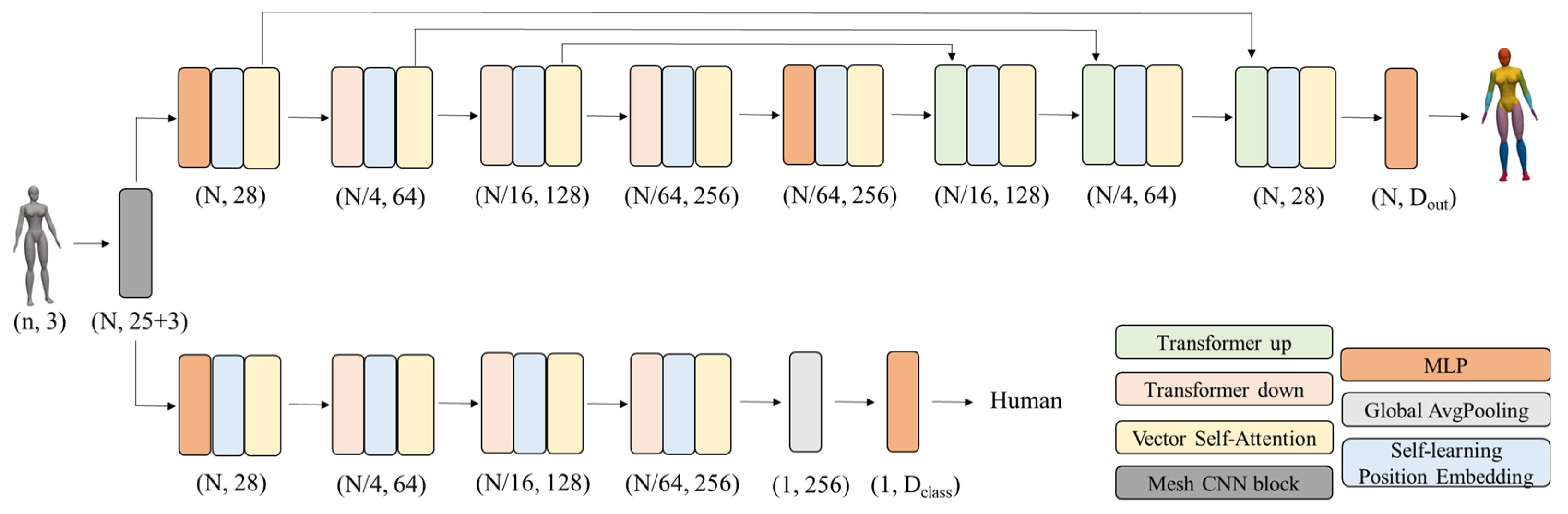
In this section, we verify the effectiveness of our method in two applications: 3D mesh model classification and surface semantic segmentation. The network design details of the experiments are shown in
Figure 4. We also have done ablation experiments for the sampling method, for the related function, and for the position encoding. We also tried different parameters in the mesh transformer block to explore the effect of the number of transformer layers and transformer output layer dimension on the experimental results.
The experimental host configuration is NVIDIA GeForce RTX 2080 Ti graphics card, Intel(R) Core(TM) i5-9600 CPU processor, and 32G RAM.
4.1. Model Parameters
The network model is built based on the Pytorch framework with Pytorch version 1.8.1. The 3D mesh model data is first convolved by the 3D mesh convolution block, and the convolved surface window is taken with the vertex as the center, and the neighborhood range is 152 vertices close to the vertex. The vertices with the convolved surface information aggregated to the neighborhood are sampled by Poisson disk to take 10% of the points, which are then mapped to the feature space by the MLP layer and input to the 3D mesh transformer block.
4.2. Classification Experiments
4.2.1. Classification Experiments Based on SHREC15 Dataset
The SHREC15 dataset is derived from SHREC11 and SHREC14 and contains both rigid and non-rigid models. The SHREC15 dataset contains 50 categories with 24 models in each category, for a total of 1200 3D mesh models. The maximum mesh resolution in the dataset is 60,210 vertices, and the average mesh resolution is 21,141 vertices. In the ratio of 3:1, 18 3D mesh models are randomly selected from each category as the training set and the rest as the test set.
In order to verify the classification effect of MixFormer proposed in this paper, this paper compares the traditional manual feature-based classification method SPH with the 3D convolution-based classification methods MeshNet and MeshCNN. The accuracy and parametric number comparison of each method for classification in the SHREC15 dataset are given in
Table 1.
Due to the large number of classes included in SHREC15, only the class classification accuracies and the average accuracy of each method for all real columns for 11 of these models are shown in
Table 1. It can be seen that the classification effect of the MixFormer proposed in this paper is better than other comparison methods, and the classification accuracy is 96.7%, which is 5 percentage points better than the optimal method MeshCNN among the comparison methods. This shows that the MixFormer proposed in this paper does have a good ability to learn features on 3D grid models and can achieve good classification results without deep network architecture
Table 2 compares the time and space complexity of the methods in this paper with those of other classification methods. The column Parmas shows the total number of parameters of the network, and the column FLOPs shows the number of floating point operations performed on each input sample, representing the spatial and temporal complexity, respectively. By learning local feature information through the front 3D grid convolution module and establishing dependencies between features through the 3D grid transformer, MixFormer has a stronger feature learning capability, so good learning results can be achieved without stacking multiple layers and with less computational overhead.
4.2.2. Classification Results Based on the Manifold40 Dataset
Manifold40 [
46] is derived from the ModelNet40 dataset, which is a new dataset contributed by Hu et al. after repairing the models in ModelNet40 to tight manifolds. In the Manifold40 dataset, 12,300 models with 40 categories are included. Manifold40 is more challenging due to the reconstruction error and simplification distortion in the Manifolds dataset.
To further validate the classification effect of the proposed MixFormer proposed in this paper, experiment was also conducted on the Manifold40 dataset and compared with the vertex-based methods: PointNet++ and PCT, and the mesh feature-based methods: MeshNet, MeshWalker, and SubdivNet. The accuracy of the classification of each method on the Manifold40 dataset is given in
Table 3.
From the comparison of the point cloud methods, it can be seen that the transformer-based PCT method works better than the PointNet++ based on multilayer convolutional networks, which implies that it may be important to obtain the dependencies of global features by introducing the transformer structure. From the comparison applied to the 3D grid model, it can be seen that the method in this paper improves by 2.1 percentage points over the SubdivNet method, which is the best among the compared methods, further indicating that the self-supervised convolutional architecture proposed by the method in this paper can learn the 3D mesh model features better.
4.3. Semantic Segmentation Experiments
To validate the feature learning effect of the proposed MixFormer in this paper, we used 370 models from SCAPE, FAUST, MIT, and Adobe Fuse as training data and 18 models from the human category in the SHREC07 dataset as test data. All models were segmented by Maron [
49] et al. into eight categories of labels: head, torso, thigh, forearm, hand thigh, calf, and foot.
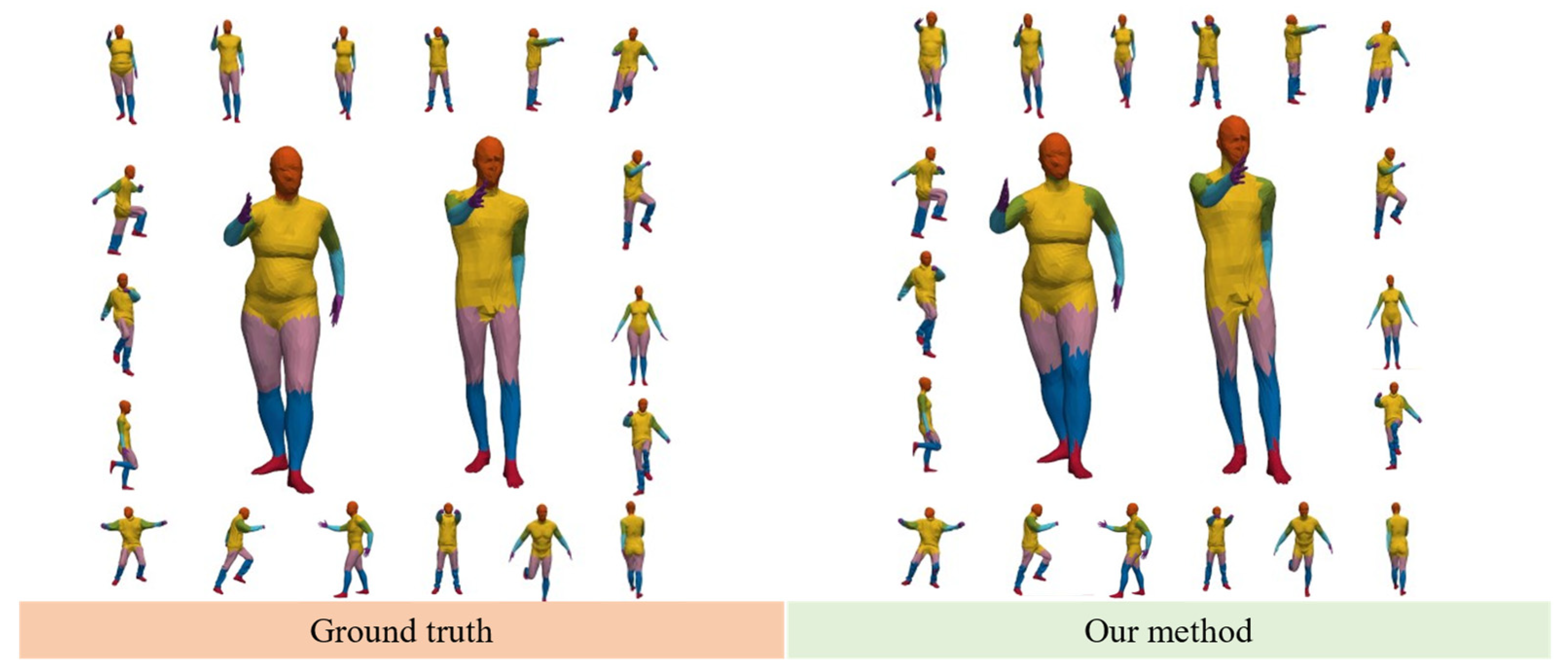
We combined the main module of MixFormer with the U-Net network to use the acquired model features for downstream tasks, such as semantic segmentation. Limited by the memory size of the graphics card, we first downsampled the model to 1024 local surfaces during the training process, and then predicted the human model. The semantic segmentation effect is shown in
Figure 5.
From the segmentation visualization results, it can be seen that the proposed MixFormer has good feature extraction ability and the ability to establish inter-feature dependencies, and can clearly delineate all parts of the human body and achieve good segmentation results. On the sampled model, mIoU is 0.849. However, some errors do exist at the joint demarcation line, which may be due to the fact that the marker of the model is not particularly fine and the joint demarcation line is difficult to define from the semantic point of view.
4.4. Ablation Experiments
To verify the effectiveness of the sampling method in MixFormer and the feature extraction method in transformer block, the following sets of ablation experiments are done for the sampling method, the correlation function, and the position encoding, respectively.
4.4.1. Sampling Method Validity
For the sampling methods, we selected random point sampling, farthest point sampling, and Poisson disk sampling for comparison. The experimental results are shown in
Table 4. Compared with the other sampling methods, the sampling points selected by the Poisson disk can better reflect the surface contour characteristics of the original 3D mesh model. As far as the classification results are concerned, the Poisson disk sampling is used for data preprocessing to obtain better classification results for the classification network, 96.7%, which is 3.6 percentage points higher than the optimal method of farthest point sampling among the compared methods.
4.4.2. Related Function
In the scalar transformer, the similarity is often calculated by dot product operation. In this paper, we adopt a vector transformer, which uses addition, subtraction, Hadamard product, or splicing as the correlation function, and obtains the vector output by the correlation function φ, which is used to measure the similarity between vectors. The experimental results in
Table 5 show that compared with the traditional dot product operation of the scalar transformer, better classification results are often achieved by using the vector transformer, which indicates that the vector transformer may be more suitable than the scalar transformer for extracting the spatial features of the 3D mesh model. When the Hadamard product is used as the correlation function, a good classification result can be obtained with a relatively low number of parameters and arithmetic power consumption.
4.4.3. Position Encoding
For location coding, the following experiments were also conducted in this paper to compare several different location coding methods. As can be seen in
Table 6, the classification accuracy of the model is 92.79% when no location encoding is introduced. When the conventional relative location encoding is introduced, the classification accuracy of the model improves to 94.08%, indicating that location encoding can indeed model the location relationship between tokens and introduce spatial information. The classification accuracy is further hinted at when we introduce the learnable location encoding, indicating that the learnable location encoding method can indeed better model the relative location and dependency relationships among tokens. To further explore the sensitivity of each part to location encoding, we acted location encoding on the attention part and feature part separately, and the experimental results showed that the attention part was more sensitive to location encoding. In this network, the learnable location encoding acting on the attention part and feature part together can achieve the optimal feature learning effect of 96.76%, which is nearly 4% higher than that without the introduction of location encoding.
4.4.4. Number of Mesh Transformer Blocks
For the number of mesh transformer blocks, this paper tries different numbers of transformer blocks to explore their effects on the experimental results. From
Table 7, we can see that the model performs best when the number of blocks is 2. When there are fewer transformer blocks, the network may not have enough deep-learning features. When there are more transformer blocks, the number of tokens input to the deep transformer block decreases and the token semantic information is blurred, and too many parameters are also introduced, which may reduce the network performance.
4.4.5. Feature Dimensions of the Output Layer
We also tried different output layer feature dimensions to explore their effects on the model performance, and the experimental results are shown in
Table 8. The network performance is optimal when the output layer feature dimension is 256.


