Article

A Novel Intelligent Method for Fault Diagnosis of Steam Turbines Based on T-SNE and XGBoost

1
National Center for Materials Service Safety, University of Science and Technology Beijing, Beijing 100083, China
2
Innovation Group of Marine Engineering Materials and Corrosion Control, Southern Marine Science and Engineering Guangdong Laboratory (Zhuhai), Zhuhai 519080, China
3
Research Institute of Macro-Safety Science, University of Science and Technology Beijing, Beijing 100083, China
*
Author to whom correspondence should be addressed.
Algorithms 2023, 16(2), 98; https://doi.org/10.3390/a16020098
Submission received: 26 December 2022 / Revised: 4 February 2023 / Accepted: 7 February 2023 / Published: 9 February 2023
(This article belongs to the Special Issue Artificial Intelligence for Fault Detection and Diagnosis)

Abstract

:
Since failure of steam turbines occurs frequently and can causes huge losses for thermal plants, it is important to identify a fault in advance. A novel clustering fault diagnosis method for steam turbines based on t-distribution stochastic neighborhood embedding (t-SNE) and extreme gradient boosting (XGBoost) is proposed in this paper. First, the t-SNE algorithm was used to map the high-dimensional data to the low-dimensional space; and the data clustering method of K-means was performed in the low-dimensional space to distinguish the fault data from the normal data. Then, the imbalance problem in the data was processed by the synthetic minority over-sampling technique (SMOTE) algorithm to obtain the steam turbine characteristic data set with fault labels. Finally, the XGBoost algorithm was used to solve this multi-classification problem. The data set used in this paper was derived from the time series data of a steam turbine of a thermal power plant. In the processing analysis, the method achieved the best performance with an overall accuracy of 97% and an early warning of at least two hours in advance. The experimental results show that this method can effectively evaluate the condition and provide fault warning for power plant equipment.

1. Introduction

Thermal power plays an important role in power generation. Thermal power generation consumes enormous amounts of available coal energy, resulting in a shortage of coal energy. In order to conserve energy consumption, reduce pollution and protect the environment, thermal power plants should adopt advanced scientific and technological means to reduce energy efficiency loss, and strengthen research on fault diagnosis of main power generation (e.g., steam boilers and turbines) [1,2,3].
In recent years, the rapid development of information technologies, computer technologies and other new technologies has brought new progress in equipment condition monitoring and fault diagnosis [4,5]. The application of machine learning in intelligent diagnosis has achieved good results. The main machine learning algorithms include support vector machines (SVM) [6,7] and its improved algorithms, decision trees, its improved algorithms [8,9], artificial neural network (ANN), and its improved algorithms [10,11], etc. These algorithms can achieve better classification results for data sets with a large number of fault tags. Deng et al. [12] used the improved particle swarm optimization (PSO) algorithm to optimize the parameters of least squares support vector machines (LS-SVM) to construct an optimal LS-SVM classifier, which is used to classify the fault. In Sun’s research [13], a fault diagnosis method based on wavelet packet analysis and SVM was proposed. Firstly, the wavelet packet transform was used to decompose and denoise the signal, and the original fault feature vector was extracted for reconstruction. The improved SVM algorithm was used to diagnose the fault based on the new fault feature vector. Wu et al. [14] proposed a deep transfer learning method based on the hybrid domain adversarial learning (HDAL) strategy for rotating machines in nuclear power plants.
Since failure of steam turbines occurs frequently and causes huge losses in thermal plants, it is important to identify the fault in advance. Thermal power plants use big data technology to deeply mine data value [15,16,17,18], which also makes itself more optimized, safer, and more economical. The steam turbine is one of the most important equipment in thermal power plants [19,20]. A large amount of steam turbine data, such as condition monitoring data, fault data and so on, has been accumulated in power plant automation systems, which contain characteristic data about the steam turbine fault condition. Accurate fault diagnosis can find the fault in time, repair it in advance, and ensure normal production. However, due to data acquisition and artificial records, the fault records cannot be directly related to the automatic acquisition of time series data. More seriously, due to the low efficiency and low quality of manual recording, the sample data with a large number of labels cannot be directly obtained. In addition, the turbine has high reliability and is in normal operation for a long time, which makes it difficult to provide a large amount of faulty sample data. Since the signals collected by the automatic system are nonlinear and non-stationary, the fault features are often drowned by external factors such as noise and the traditional signal processing; thus, analysis technology is severely limited. Therefore, an effective method for feature extraction and fault diagnosis for steam turbines is needed for this condition.
After analyzing the recent progress, a novel fault diagnosis method based on t-distribution stochastic neighborhood embedding (t-SNE), K-means clustering, synthetic minority over-sampling technique (SMOTE) and extreme gradient boosting (XGBoost) is proposed in this paper. Since the vibration signal collected by samplers had a high dimensional feature and the data could not be visualized, t-SNE was used to map the high-dimensional data to the low-dimensional space. Most of the data collected from the thermal plant was unlabeled, so the data clustering method of K-means was used in the low-dimensional space to distinguish the fault data from the normal data for automatic fault identification. The imbalance problem in the data was processed by the SMOTE algorithm to obtain the steam turbine characteristic data set with fault labels. Finally, the XGBoost algorithm was used to solve this multi-classification problem. When the steam turbines were detected by the trained model in this paper, the prediction information fed back to the thermal power plant immediately. This early warning information for a predictive failure will give the thermal power plant enough time to deal with the problems in advance. During this time, the plant could use other methods to reasonably determine when to take action. Compared with the above literature, the differences between the proposed method and other studies are shown in Table 1. The main objective of the proposed method was to develop a novel procedure for actual power plant data.
The rest of this paper is organized as follows. Section 2 discusses methods. Section 2.1 introduces and discusses the performance indicator extraction based on t-SNE and K-means. Section 2.2 introduces the imbalanced data recognition model based on SMOTE and XGBoost. A model evaluation method is presented in Section 2.3. Section 3 presents the data experiment and results and discussion of the proposed method. Finally, conclusions are drawn in Section 4.

2. Methods

2.1. Performance Indicator Extraction Based on t-SNE and K-Means

The t-SNE algorithm is a nonlinear dimensionality reduction algorithm that maps multi-dimensional data into two or more dimensions by the similarity of high-dimensional data [21,22]. It has been applied to many fields, including image processing [23], genetics [24], and materials science [25]. In this paper, the input of t-SNE is signal features extracted by data acquisition equipment. According to the similarity of signal features, these features are further reduced. The main algorithm is as follows and the source code of the t-SNE algorithm is in Appendix A.
(1) The conditional probability of distribution p j | i between the corresponding data x i and x j in the high-dimensional space is calculated to represent the similarity between the data. The high-dimensional data, x i and x j , correspond to the mapping points y i and y j in a low dimension and q j | i is their similar conditional probability distribution. The initial value is Y 0 = y 1 y 2 y n . p j | i and q j | i are calculated as follows.
p j | i = exp ( x i x j 2 / 2 σ i 2 ) k i exp ( x i x k 2 / 2 σ i 2 )
q j | i = exp ( y i y j 2 ) k i exp ( y i y k 2 )
where σ i is the Gaussian distribution variance centered on x i .
(2) Calculating the joint probability density p i j of high dimensional samples.
p i j = p j | i + p i | j 2 n
(3) Calculating the joint probability density q i j of the low dimensional samples.
q i j = 1 + y i y j 2 1 k l 1 + y k y l 2 1
(4) Calculating the loss function C and its gradient. C is defined by the Kullback–Leibler (KL) distance to evaluate the similarity degree of joint probability density p i j and q i j .
C = KL = i j p i j log p i j q i j
δ C δ y i = 4 j p i j q i j y i y j 1 + y i y j 2 1
(5) Iterative updating.
Y t = Y t 1 + η δ C δ y + α t Y t 1 Y t 2
where t is the number of iterations, η is the learning rate, and α · is the momentum factor.
(6) Returning to (4) and (5) until the number of iterations is reached.
After obtaining the low-dimensional data output by the t-SNE algorithm, the K-means clustering algorithm [26] was used to classify the data into two categories. This algorithm is used to classify fault dangerous intervals. When a single fault hazardous interval is identified, the data is divided into fault data and normal data. However, the lack of failure records leads to an imbalance problem.

2.2. Imbalanced Data Recognition Model Based on SMOTE and XGBoost

Sampling methods are very popular for balancing the class distribution. Over- and under-sampling methodologies have received considerable attention to counteract the effect of imbalanced data sets. The SMOTE algorithm is simple and efficient, has good anti-noise ability, and can improve the generalization of the model [27,28]. The formal procedure is as follows.
The minority class is over-sampled by taking each minority class sample and inserting synthetic examples along the line segments connecting any/all of the k minority class nearest neighbors. Depending on the amount of over-sampling required, neighbors are randomly selected from the k nearest neighbors. Synthetic samples are generated as follows: take the difference between the feature vector of sample and its nearest neighbor; multiply this difference by a random number between 0 and 1, and add it to the feature vector under consideration. This results in the selection of a random point along the line segment between two specific features. This approach effectively forces the decision region of the minority class to become more general [29].
Boosting is a machine learning technique that can be used for regression and classification problems. It generates a weak learner at each step and accumulates them in the overall model. If the weak learner for each step is based on the gradient direction of the loss function, it can be called gradient boosting decision tree (GBDT) [30]. The difference with GBDT is that only the first derivative of the loss function is used to compute the objective function. The XGBoost approximates the loss function using the second order Taylor expansion. The main algorithm is as follows and the source code of the XGBoost algorithm is in Appendix A.
Assume that a data set is D = x i , y i D = m , x i R n , y i R , then we obtain n observations with m features each and with a corresponding variable y . Let y ^ be defined as a result given by an ensemble represented by the generalized model as follows:
y ^ i = ϕ x i = k = 1 K f k x i , f k F
where f k is a regression tree, and f k x i represents the score given by the k-th tree to the i-th observation in data. In order to functions f k , the following regularized objective function should be minimized:
L ϕ = i l y ^ i , y i + k Ω f k
where l is the loss function. To prevent too large complexity of the model, the penalty term Ω is included as follows:
Ω f k = γ T + 1 2 λ ω 2
where γ and λ are parameters controlling penalty for the number of leaves T and magnitude of leaf weights ω respectively. The purpose of Ω f k is to prevent over-fitting and to simplify models produced by this algorithm.
An iterative method is used to minimize the objective function. The objective function that minimized in j-th iterative to add f j is:
L j = i = 1 n l y i , y ^ i t 1 + f j x i + Ω f j
Equation (11) can be simplified by using the Taylor expansion. Then, a formula can be derived for loss reduction after the tree split from a given node:
L s p l i t = 1 2 i I L g i 2 i I L h i + λ + i I R g i 2 i I R h i + λ i I g i 2 i I h i + λ γ
where I is a subset of the available observations in the current node and I L , I R are subsets of the available observations in the left and right nodes after the split. The functions g i and h i are defined as follows:
g i = y ^ j 1 l y i , y ^ j 1
h i = y ^ j 1 2 l y i , y ^ j 1
The XGBoost algorithm has many advantages: it prevents over-fitting by increasing the complexity and compression of the loss function; it optimizes the number of iterations through cross-validation; and it improves the computational efficiency of the model through parallel processing. This algorithm is implemented in the “xgboost” package for the “Python” language provided by the creators of the algorithm.

2.3. Model Assessment Method

The confusion matrix [31] is a classical method for evaluating the results of classification models:
C q = N 11 N 12 N 1 k N 21 N 22 N 2 k N k 1 N k 2 N k k
where N i j represents the probability that class i is divided into class j on the verification set.
Accuracy, recall, and F1-score [32] play a role in the evaluation of the classification model. Through these complementary evaluation indexes, with the results of the confusion matrix, the algorithm model can be evaluated, optimized and screened, and the optimal algorithm model suitable for the data can be obtained.
Accuracy refers to the ratio of the predicted correct number in the test results of the test set to the total number of samples, which is expressed as follows.
A c c u r a c y = i N i i i j N i j
The precision of class i indicates the ratio between the number of class i predicted correctly and the number of class i predicted in the test set results, which is expressed as follows:
P r e c i s i o n = N i i j N i j
Recall refers to the ratio between the number of correct class i predicted in the test results of the test set and the number of class i. The equation is as follows:
R e c a l l = N i i i N i j
F1-score is calculated by precision and recall. Since these two values are not intuitive enough, they are more intuitive after conversion. The larger the value, the better the result. The formula is as follows:
F 1 = 2 P R P + R
where P is the accuracy and R represents the recall rate.
Through the accuracy rate, recall rate, and F1-score, which can reflect the quality of classification results, we can adjust and optimize the classification model.
To better understand the proposed fault diagnosis of the steam turbine process, we summarize the main procedures as follows.
Step 1: Extraction of performance indicators. The t-SNE algorithm is used for dimension reduction. Then, cluster analysis is performed on the low-dimensional data. With the fault records, the fault data and normal data of the clustering result are distinguished.
Step 2: Imbalanced data detection model. The imbalance problem in the data is processed by the SMOTE algorithm. We used the XGBoost algorithm to solve this multiclassification problem.
Step 3: Model evaluation method. The confusion matrix is used to evaluate the results of classification models.
Figure 1 shows a schematic diagram of the proposed fault diagnosis of the steam turbine process in this paper.

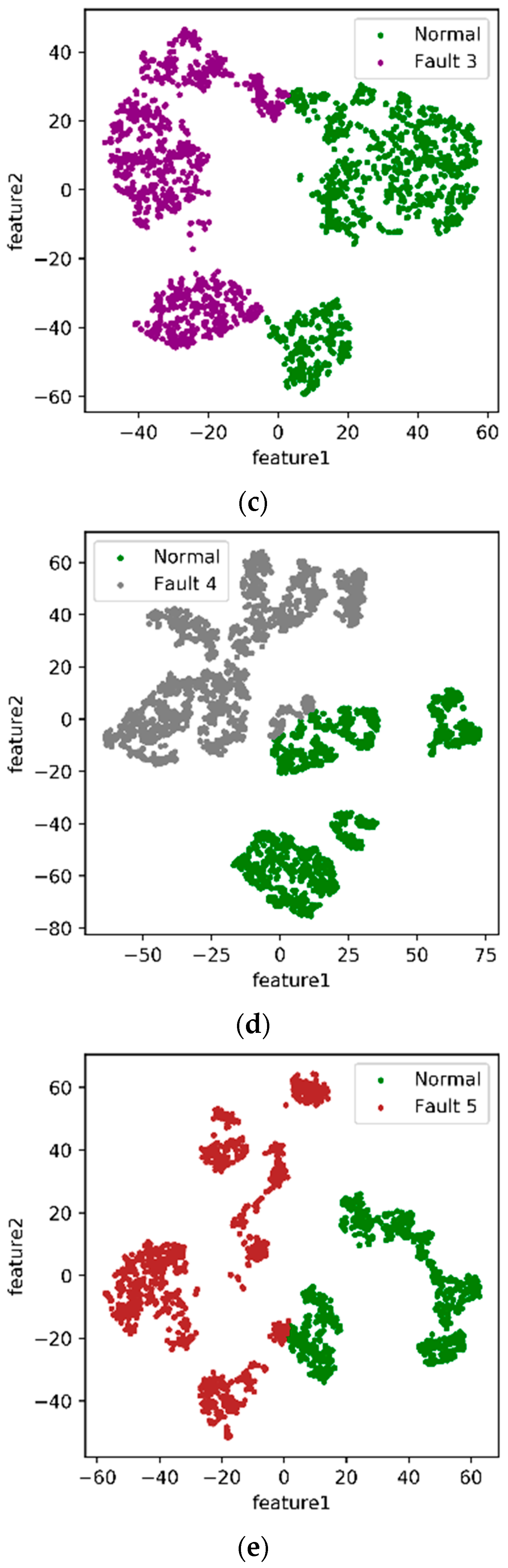
3. Experiments, Results and Discussion

3.1. Introduction of Data Set

The data set in this paper was derived from the time series data of Steam Turbine 2 in a thermal power plant in China. The data set include the following two parts.
(1) One was from the supervisory control and data acquisition (SCADA) system. The original sampling period of the SCADA system was less than one millisecond. The data set was the interval sampling data of every one second.
(2) The other was the fault information from the manual record and the system application and product (SAP). The fault information mainly came from the manual record of the power plant, including the fault content and the recorded time. However, some of the fault information was not part of the equipment operation faults and could not be effectively identified by the automated acquisition system. Therefore, in this paper, the fault information was filtered.
After excluding measurement points with severe data loss or no data records, the steam turbine data set contained 34 variables, such as the time stamp, operating condition parameters and status parameters. The acquisition time was eight months, and the size of the effect data was approximately 340,000.
Table 2 shows the statistical information of the steam turbine data set. In addition, more detailed information of the data set can be seen in Appendix B, Table A1.
The fault information was obtained from the fault records manually recorded by the power plant, including the fault content and recording time. Since some fault records were not plant operation faults and could not be effectively identified by the data, the available fault information was screened. The fault records selected for use are shown in Table 3.

3.2. Setting Labels for Different or Normal Faults

We used the fault detection time in the data record to determine the time that the fault occurred. The data of 8~24 h before and after each fault record of the steam turbine were intercepted for analysis. First, the t-SNE algorithm described in the previous section was adopted to map the 34-dimensional data to a two-dimensional space. Then, the K-means clustering method was used to separate the fault data from the normal data. The processing results of the algorithm are visualized in Figure 2. Green data points represent normal data, and other colors represent different fault data points.
The time-series data after clustering was compared to fault records to distinguish fault data from normal data. As shown in Figure 3, each figure is a data graph of different faults arranged by time. In the figure, the time of the red line is the actual time recorded for the five types of faults.
Table 4 shows the information of failure data for five types. Compared to the time of fault records, it can be seen that this method can distinguish fault data and normal data of steam turbines, and it has a certain predictive ability.

3.3. Dealing with Data Imbalance

After labelling the data, the problem to be solved was the data imbalance.
The total number of fault data was 5118 and the number of normal data was 335,350. The ratio of normal data to faulty data was approximately 67:1, which is a very high imbalance. The imbalance needed to be processed before building a classification model. Immediate imbalance processing of this data set could introduce noise, which would affect the accuracy of subsequent classification algorithms.
The normal data were sampled in sections, and the data of one day every four days were extracted and reassembled into the normal data. The SMOTE algorithm was used to deal with the unbalanced data of the newly formed data, and the resulting sample data set is shown in Table 5.

3.4. Test Results

After optimizing the data imbalance in the previous section, the XGBoost algorithm could be used for fault diagnosis. The data set was divided into a training set and a test set and divided according to the ratio of 3:7. The results of the confusion matrix are shown in Table 6.
To better calculate the performance of the model, precision, recall rate and F1-score were calculated, and the calculation results are shown in Table 7.
Table 6 and Table 7 show the classification results of the model for five faults of the steam turbine. As is well-known, for a classification model, if precision, recall and F1-score have higher values at the same time without considering other factors, the model is considered to have better performance. The model based on the XGBoost classifier had high accuracy in fault diagnosis of steam turbines and could identify the different types of faults.

3.5. Results and Discussion

In this paper, we developed a novel procedure for the actual data of the power plant, and obtained the expected results for the power plant. In order to further illustrate the superiority of the proposed method in this paper over other methods, it is necessary to discuss the following issues.
(1) Computational efficiency.
The research object of this paper was a power plant’s big data, so the complexity of the algorithm was one of the important issues to be considered. The complexity of the T-SNE algorithm used in the research method of this paper is large. In general, applying the T-SNE algorithm for dimensionality reduction for a data set of millions of samples may take several hours. The number of samples calculated in this paper was about 340,000, and the training time of the model including the dimensionality reduction algorithm was less than one hour. Such computational efficiency is perfectly acceptable for an enterprise-level data application system. In addition, since the probability of serious faults in power plant enterprises is often low, we generally recommend that power plants update the training model every six months with new data, and the time to update the model here is at most a few hours. For the calculation time of the final classification model, achievement of the real-time effect can be considered (generally no more than 1 s).
(2) Comparison with other algorithms.
The purpose of this research paper was to develop a procedure of fault diagnosis and prediction for the power plant data. For the data dimensionality reduction algorithm, we chose the t-SNE algorithm. In the research process, we also compared a principal component analysis (PCA) algorithm at the same time. Although, the PCA method had a faster computational speed, it was still less effective than nonlinear dimensionality reduction algorithms, such as t-SNE, for complex data of the power plant due to the linear dimensionality reduction method [33].
For the final classification algorithm, in addition to the XGBoost algorithm, we also compared algorithms such as SVM and random forest (RF). From the application effect of the data in this paper, the computational results of the XGBoost algorithm and the RF algorithm were better than SVM; moreover, considering that the XGBoost algorithm borrows from RF and can support column sampling processing, which can not only reduce overfitting, but also reduce computational effort [34], the XGBoost algorithm was finally chosen in this paper.
(3) Improvement of the algorithm.
For a fault diagnosis and prediction system that is really applied to the power plant, the most important purpose was to be able to detect and warn about the dangerous faults in advance based on the large historical data. In this paper, the algorithm was trained with more than 300,000 samples of data for nearly eight months, and the algorithm had some limitations. However, in the actual application system, we used more than seven years of historical data of the power plant to train the used model, which proved to have a good application effect.
Furthermore, in addition to the application data set in this paper, we also validated the pneumatic feed pump data set for this power plant. The results also showed that the method proposed in this paper was also applicable to other equipment in the power plant. In general, the accuracy of 90% of the actual data can meet the needs of the enterprise management. Therefore, the research algorithm in this paper has been practically applied in the power plant and has achieved satisfactory results.

4. Conclusions

A model based on t-SNE and XGBoost was proposed to detect the early failure of steam turbines. The model with high accuracy was verified by the data of steam turbine units of thermal power plants in China.
(1) The uncertainty problem of feature extraction in the unlabeled data set was solved using t-SNE and K-means. This method can distinguish fault data and normal data, and it has a certain foresight because it can distinguish the time when the fault occurs, which is earlier than the fault record of manual inspection, making it more suitable for practical application in fault diagnosis of steam turbines.
(2) The problem of data imbalance caused by fewer fault records was solved by using the SMOTE algorithm, which is of great significance to the fault diagnosis of the steam turbine and other mechanical equipment with fewer faulty samples.
(3) In the identification of new data, the accuracy and other indicators of the model based on XGBoost reached more than 97%, which shows that this method has high value in turbine fault diagnosis.

Author Contributions

Conceptualization, L.Z. and X.W.; methodology, L.Z. and X.W.; software, X.W.; validation, Z.L., L.Z. and X.W.; formal analysis, L.Z.; investigation, X.W.; resources, L.Z.; data curation, L.Z.; writing—original draft preparation, X.W.; writing—review and editing, Z.L. and L.Z.; supervision, L.Z.; project administration, L.Z.; funding acquisition, L.Z. All authors have read and agreed to the published version of the manuscript.

Funding

This research was supported by Innovation Group Project of Southern Marine Science and Engineering Guangdong Laboratory (Zhuhai) of China (No. 311021013), National Natural Science Foundation of China (No. 51775037), and Fundamental Research Funds for Central Universities of China (No. FRF-BD-18-001A).

Institutional Review Board Statement

Not applicable.

Informed Consent Statement

Not applicable.

Data Availability Statement

Data is contained within the article.

Acknowledgments

The authors thank the National Center for Materials Service Safety for support of the simulation and data platform.

Conflicts of Interest

The authors declare no conflict of interest.

Appendix A

The following source code for reference is the t-SNE algorithm.
Algorithm A1. T-SNE algorithm.
#!/usr/bin/env python
    # coding: utf-8
    
    import os
    import sys
    os.chdir (os.path.split (os.path.realpath (sys.argv [0]))[0])
    
    import numpy
    from numpy import *
    import numpy as np
    
    from sklearn.manifold import TSNE
    from sklearn.datasets import load_iris
    from sklearn.decomposition import PCA
    import matplotlib.pyplot as plt
    
    import pandas as pd
    
    df1 = pd.read_excel (‘D:/data/gz5.xlsx’)
    
    df1.label.value_counts ()
    
    def get_data (data):
                X = data.drop (columns = [‘time’, ‘label’]).values
                y = data.label.values
                n_samples, n_features = X.shape
                return X, y, n_samples, n_features
    
    X1, y1, n_samples1, n_features1 = get_data (df1)
    
    X_tsne = TSNE (n_components = 2,init = ‘pca’, random_state = 0).fit_transform (X1)
    
    def plot_embedding (X, y, title = None):
                x_min, x_max = np.min(X, 0), np.max(X, 0)
                X = (X − x_min) / (x_max − x_min)
    
                plt.figure ()
                ax = plt.subplot (111)
                for i in range (X.shape [0]):
                            plt.text (X [i, 0], X [i, 1], ‘.’,
                                                color = plt.cm.Set1 (y[i] * 3/10.),
                                                fontdict = {‘weight’: ‘bold’, ‘size’: 9})
                plt.xticks ([]), plt.yticks ([])
                if title is not None:
                            plt.title (title)
    
    
    plot_embedding (X_tsne, y1)
    
    from sklearn.cluster import KMeans
    from sklearn.externals import joblib
    from sklearn import cluster
    
    estimator = KMeans (n_clusters = 2)
    
    res = estimator.fit_predict (X_tsne)
    
    lable_pred = estimator.labels_
    
    centroids = estimator.cluster_centers_
    
    inertia = estimator.inertia_
    
    from pandas import DataFrame
    XA = DataFrame (res)
    XA.to_csv (‘D:/data/gz5out.csv’)
The following source code for reference is the XGBoost algorithm.
Algorithm A2. XGBoost algorithm.
#!/usr/bin/env python
    # coding: utf-8
    
    from xgboost import plot_importance
    from matplotlib import pyplot as plt
    
    import xgboost as xgb
    from sklearn.model_selection import train_test_split
    from sklearn.metrics import accuracy_score
    import numpy as np
    import pandas as pd
    from xgboost.sklearn import XGBClassifier
    
    # load data
    data = pd.read_csv (‘D:/data/suanfa/kyq.csv’)
    x, y = data.loc [:,data.columns.difference ([‘label’])].values, data [‘label’].values
    x_train, x_test, y_train, y_test = train_test_split (x, y, test_size = 0.3)
    
    data.label.value_counts ()
    
    params ={‘learning_rate’: 0.1,
                            ‘max_depth’: 2,
                            ‘n_estimators’:50,
                            ‘num_boost_round’:10,
                            ‘objective’: ‘multi:softprob’,
                            ‘random_state’: 0,
                            ‘silent’:0,
                            ‘num_class’:6,
                            ‘eta’:0.9
                    }
    
    model = xgb.train (params, xgb.DMatrix (x_train, y_train))
    y_pred = model.predict (xgb.DMatrix (x_test))
    yprob = np.argmax (y_pred, axis = 1) # return the index of the biggest pro
    
    model.save_model (‘testXGboostClass.model’)
    
    yprob = np.argmax (y_pred, axis = 1) # return the index of the biggest pro
    
    predictions = [round (value) for value in yprob]
    
    # evaluate predictions
    accuracy = accuracy_score(y_test, predictions)
    print (“Accuracy: %.2f%%” % (accuracy * 100.0))
    
    plot_importance (model)
    plt.show ()
    
    xgb1 = XGBClassifier (
                            learning_rate = 0.1,
                            n_estimators = 20,
                            max_depth = 2,
                            num_boost_round = 10,
                            random_state = 0,
                            silent = 0,
                            objective = ‘multi:softprob’,
                            num_class = 6,
                            eta = 0.9
                            )
    
    xgb1.fit (x_train, y_train)
    
    y_pred1 = xgb1.predict_proba (x_test)
    
    yprob1 = np.argmax (y_pred1, axis = 1) # return the index of the biggest pro
    
    from sklearn.metrics import confusion_matrix
    confusion_matrix (y_test.astype (‘int’), yprob1.astype (‘int’))
    
    from sklearn.metrics import classification_report
    print (‘Accuracy of Classifier:’,xgb1.score (x_test, y_test.astype (‘int’)))
    print (classification_report (y_test.astype (‘int’), yprob1.astype (‘int’)))

Appendix B

Table A1. Variable name.
No.Description
F0Time stamp
F1Turbine Speed
F2Main Steam Pressure
F3Reheat Steam Pressure
F4Main Steam Temp
F5Bearing Bushing 11
F6Bearing Bushing 12
F7Bearing Bushing 21
F8Bearing Bushing 22
F9Bearing Bushing 31
F10Bearing Bushing 32
F11Bearing Bushing 41
F12Bearing Bushing 42
F13Bearing Bushing 51
F14Bearing Bushing 61
F15Bearing Vibration 1X
F16Bearing Vibration 1Y
F17Bearing Vibration 1Z
F18Bearing Vibration 2X
F19Bearing Vibration 2Y
F20Bearing Vibration 2Z
F21Bearing Vibration 3X
F22Bearing Vibration 3Y
F23Bearing Vibration 3Z
F24Bearing Vibration 4X
F25Bearing Vibration 4Y
F26Bearing Vibration 4Z
F27Bearing Vibration 5X
F28Bearing Vibration 5Y
F29Bearing Vibration 5Z
F30Bearing Vibration 6X
F31Bearing Vibration 6Y
F32Bearing Vibration 6Z
F33Turbine Differential Expansion
F34Rotor Eccentricity

References

  1. Yu, J.; Jang, J.; Yoo, J.; Park, J.H.; Kim, S. A fault isolation method via classification and regression tree-based variable ranking for drum-type steam boiler in thermal power plant. Energies 2018, 11, 1142. [Google Scholar] [CrossRef]
  2. Madrigal, G.; Astorga, C.M.; Vazquez, M.; Osorio, G.L.; Adam, M. Fault diagnosis in sensors of boiler following control of a thermal power plant. IEEE Lat. Am. Trans. 2018, 16, 1692–1699. [Google Scholar] [CrossRef]
  3. Wu, Y.; Li, W.; Sheng, D.; Chen, J.; Yu, Z. Fault diagnosis method of peak-load-regulation steam turbine based on improved PCA-HKNN artificial neural network. Proc. Inst. Mech. Eng. O J. Risk Reliab. 2021, 235, 1026–1040. [Google Scholar] [CrossRef]
  4. Cao, H.; Niu, L.; Xi, S.; Chen, X. Mechanical model development of rolling bearing-rotor systems: A review. Mech. Syst. Signal Process. 2018, 102, 37–58. [Google Scholar] [CrossRef]
  5. Xu, Y.; Zhen, D.; Gu, J.; Rabeyee, K.; Chu, F.; Gu, F.; Ball, A.D. Autocorrelated Envelopes for early fault detection of rolling bearings. Mech. Syst. Signal Process. 2021, 146, 106990. [Google Scholar] [CrossRef]
  6. Kazemi, P.; Ghisi, A.; Mariani, S. Classification of the Structural Behavior of Tall Buildings with a Diagrid Structure: A Machine Learning-Based Approach. Algorithms 2022, 15, 349. [Google Scholar] [CrossRef]
  7. Shi, Q.; Zhang, H. Fault Diagnosis of an Autonomous Vehicle With an Improved SVM Algorithm Subject to Unbalanced Datasets. IEEE Trans. Ind. Electron. 2021, 68, 6248–6256. [Google Scholar] [CrossRef]
  8. Zhang, P.; Gao, Z.; Cao, L.; Dong, F.; Zhou, Y.; Wang, K.; Zhang, Y.; Sun, P. Marine Systems and Equipment Prognostics and Health Management: A Systematic Review from Health Condition Monitoring to Maintenance Strategy. Machines 2022, 10, 72. [Google Scholar] [CrossRef]
  9. Li, X.; Wu, S.; Li, X.; Yuan, H.; Zhao, D. Particle swarm optimization-Support Vector Machine model for machinery fault diagnoses in high-voltage circuit breakers. Chin. J. Mech. Eng. 2020, 33, 6. [Google Scholar] [CrossRef]
  10. Zan, T.; Liu, Z.; Wang, H.; Wang, M.; Gao, X.; Pang, Z. Prediction of performance deterioration of rolling bearing based on JADE and PSO-SVM. Proc. Inst. Mech. Eng. C J. Mech. Eng. Sci. 2020, 235, 1684–1697. [Google Scholar] [CrossRef]
  11. Fink, O.; Wang, Q.; Svensen, M.; Dersin, P.; Lee, W.-J.; Ducoffe, M. Potential, challenges and future directions for deep learning in prognostics and health management applications. Eng. Appl. Artif. Intell. 2020, 92, 103678. [Google Scholar] [CrossRef]
  12. Deng, W.; Yao, R.; Zhao, H.; Yang, X.; Li, G. A novel intelligent diagnosis method using optimal LS-SVM with improved PSO algorithm. Soft Comput. 2019, 23, 2445–2462. [Google Scholar] [CrossRef]
  13. Sun, H.; Zhang, L. Simulation study on fault diagnosis of power electronic circuits based on wavelet packet analysis and support vector machine. J. Electr. Syst. 2018, 14, 21–33. [Google Scholar]
  14. Wang, Z.; Xia, H.; Yin, W.; Yang, B. An improved generative adversarial network for fault diagnosis of rotating machine in nuclear power plant. Ann. Nucl. Energy 2023, 180, 109434. [Google Scholar] [CrossRef]
  15. Kang, C.; Wang, Y.; Xue, Y.; Mu, G.; Liao, R. Big Data Analytics in China’s Electric Power Industry. IEEE Power Energy Mag. 2018, 16, 54–65. [Google Scholar] [CrossRef]
  16. Ma, Y.; Huang, C.; Sun, Y.; Zhao, G.; Lei, Y. Review of Power Spatio-Temporal Big Data Technologies for Mobile Computing in Smart Grid. IEEE Access 2019, 7, 174612–174628. [Google Scholar] [CrossRef]
  17. Lai, C.S.; Locatelli, G.; Pimm, A.; Wu, X.; Lai, L.L. A review on long-term electrical power system modeling with energy storage. J. Clean. Prod. 2021, 280, 124298. [Google Scholar] [CrossRef]
  18. Dhanalakshmi, J.; Ayyanathan, N. A systematic review of big data in energy analytics using energy computing techniques. Concurr. Comput. Pract. Exp. 2021, 34, e6647. [Google Scholar] [CrossRef]
  19. Li, W.; Li, X.; Niu, Q.; Huang, T.; Zhang, D.; Dong, Y. Analysis and Treatment of Shutdown Due to Bearing Vibration Towards Ultra-supercritical 660MW Turbine. IOP Conf. Ser. Earth Environ. Sci. 2019, 300, 42006–42008. [Google Scholar] [CrossRef]
  20. Ashraf, W.M.; Rafique, Y.; Uddin, G.M.; Riaz, F.; Asin, M.; Farooq, M.; Hussain, A.; Salman, C.A. Artificial intelligence based operational strategy development and implementation for vibration reduction of a supercritical steam turbine shaft bearing. Alex. Eng. J. 2022, 61, 1864–1880. [Google Scholar] [CrossRef]
  21. van der Maaten, L.; Hinton, G. Visualizing Data using t-SNE. J. Mach. Learn. Res. 2008, 9, 2579–2605. [Google Scholar]
  22. Gisbrecht, A.; Schulz, A.; Hammer, B. Parametric nonlinear dimensionality reduction using kernel t-SNE. Neurocomputing 2015, 147, 71–82. [Google Scholar] [CrossRef] [Green Version]
  23. Wang, H.-H.; Chen, C.-P. Applying t-SNE to Estimate Image Sharpness of Low-cost Nailfold Capillaroscopy. Intell. Autom. Soft Comput. 2022, 32, 237–254. [Google Scholar] [CrossRef]
  24. Xu, X.; Xie, Z.; Yang, Z.; Li, D.; Xu, X. A t-SNE Based Classification Approach to Compositional Microbiome Data. Front. Genet. 2020, 11, 620143. [Google Scholar] [CrossRef]
  25. Yi, C.; Tuo, S.; Tu, S.; Zhang, W. Improved fuzzy C-means clustering algorithm based on t-SNE for terahertz spectral recognition. Infrared Phys. Technol. 2021, 117, 103856. [Google Scholar] [CrossRef]
  26. Gutierrez-Lopez, A.; Gonzalez-Serrano, F.-J.; Figueiras-Vidal, A.R. Optimum Bayesian thresholds for rebalanced classification problems using class-switching ensembles. Pattern Recognit. 2023, 135, 109158. [Google Scholar] [CrossRef]
  27. Arora, J.; Tushir, M.; Sharma, K.; Mohan, L.; Singh, A.; Alharbi, A.; Alosaimi, W. MCBC-SMOTE: A Majority Clustering Model for Classification of Imbalanced Data. CMC-Comput. Mater. Contin. 2022, 73, 4801–4817. [Google Scholar] [CrossRef]
  28. Kumar, A.; Gopal, R.D.; Shankar, R.; Tan, K.H. Fraudulent review detection model focusing on emotional expressions and explicit aspects: Investigating the potential of feature engineering. Decis. Support Syst. 2022, 155, 113728. [Google Scholar] [CrossRef]
  29. Guo, S.; Chen, R.; Li, H.; Zhang, T.; Liu, Y. Identify Severity Bug Report with Distribution Imbalance by CR-SMOTE and ELM. Int. J. Softw. Eng. Knowl. Eng. 2019, 29, 139–175. [Google Scholar] [CrossRef]
  30. Duan, G.; Han, W. Heavy Overload Prediction Method of Distribution Transformer Based on GBDT. Int. J. Pattern Recognit. Artif. Intell. 2022, 36, 2259014. [Google Scholar] [CrossRef]
  31. Liu, X.; Liu, W.; Huang, H.; Bo, L. An improved confusion matrix for fusing multiple K-SVD classifiers. Knowl. Inf. Syst. 2022, 64, 703–722. [Google Scholar] [CrossRef]
  32. Maldonado, S.; López, J.; Jimenez-Molina, A.; Lira, H. Simultaneous feature selection and heterogeneity control for SVM classification: An application to mental workload assessment. Expert Syst. Appl. 2020, 143, 112988. [Google Scholar] [CrossRef]
  33. Anowar, F.; Sadaoui, S.; Selim, B. Conceptual and empirical comparison of dimensionality reduction algorithms (PCA, KPCA, LDA, MDS, SVD, LLE, ISOMAP, LE, ICA, t-SNE). Comput. Sci. Rev. 2021, 40, 100378. [Google Scholar] [CrossRef]
  34. Khan, N.; Taqvi, S.A.A. Machine Learning an Intelligent Approach in Process Industries: A Perspective and Overview. ChemBioEng Rev. 2023. [Google Scholar] [CrossRef]
Figure 1. Flow chart of model construction.
Algorithms 16 00098 g001
Figure 2. Two-dimensional features of five faults. (a) Two-dimensional fusion features of Fault 1. (b) Two-dimensional fusion features of Fault 2. (c) Two-dimensional fusion features of Fault 3. (d) Two-dimensional fusion features of Fault 4. (e) Two-dimensional fusion features of Fault 5.
Algorithms 16 00098 g002aAlgorithms 16 00098 g002b
Figure 3. Time series data of five faults. (a) Clustering results of Fault 1 based on time series. (b) Clustering results of Fault 2 based on time series. (c) Clustering results of Fault 3 based on time series. (d) Clustering results of Fault 4 based on time series. (e) Clustering results of Fault 5 based on time series.
Algorithms 16 00098 g003
Table 1. Research comparison of the proposed method.
Proposed MethodOther Literatures
Data set sourceActual data from the actual plantExperimental data or numerical simulation data
Data lengthLarger (months or even years)Smaller (hours or days)
Fault labelPartly missing or being blurredIdentified by the experiment
Fault verificationBased on real faults in the plantBased on simulated faults
Iterative strategy for research Determined by the actual operation of the plantUnable to iterate
Significance of researchSolving practical problemsContinuous improvement of research algorithms
Table 2. Statistical information of the data set on steam turbines.
Data SetSample SizeTime Range
Steam turbine340,468January to August in 2018
Table 3. Five types of faults in the fault record.
No.Fault Discovery Time
13 Feb 2018 2:07
211 Feb 2018 6:19
313 Mar 2018 7:28
410 Jun 2018 7:44
57 Aug 2018 23:17
Table 4. Five types of fault data information table.
No.Start TimeEnd TimeAdvanced Time (min)
13 Feb 2018 0:143 Feb 2018 6:45113
210 Feb 2018 22:0211 Feb 2018 16:16497
312 Mar 2018 19:3213 Mar 2018 11:10716
49 Jun 2018 14:5310 Jun 2018 17:251011
57 Aug 2018 12:078 Aug 2018 6:25670
Table 5. The amount of fault data.
Original Databy SMOTE
Normal78,51378,513
Fault 13925832
Fault 2109516,823
Fault 393914,402
Fault 4159324,655
Fault 5109916,801
Ratio15:11:1
Table 6. Results of confusion matrix.
Confusion MatrixPredicted Result (%)
012345
097.060.081.090.670.370.73
10.0699.940000
21.24098.76000
32.360097.6400
40.4100099.590
50.27000099.72
Table 7. Precision, recall and F1-score results.
Fault LabelPrecisionRecall RateF1-Score
099.18%96.80%97.98%
198.74%100.00%99.37%
294.54%99.02%97.07%
396.52%97.63%97.07%
498.52%99.70%99.11%
596.58%99.72%98.13%
Disclaimer/Publisher’s Note: The statements, opinions and data contained in all publications are solely those of the individual author(s) and contributor(s) and not of MDPI and/or the editor(s). MDPI and/or the editor(s) disclaim responsibility for any injury to people or property resulting from any ideas, methods, instructions or products referred to in the content.

