

Image Quality Assessment for Gibbs Ringing Reduction


School of Electrical and Electronic Engineering, University College Dublin, D04 V1W8 Dublin, Ireland
*
Author to whom correspondence should be addressed.
Algorithms 2023, 16(2), 96; https://doi.org/10.3390/a16020096
Submission received: 14 December 2022
/
Revised: 7 February 2023
/
Accepted: 8 February 2023
/
Published: 9 February 2023
(This article belongs to the Collection Traditional and Machine Learning Methods to Solve Imaging Problems)
Abstract
:Gibbs ringing is an artefact that is inevitable in any imaging modality where the measurement is Fourier band-limited. It impacts the quality of the image by creating a ringing appearance around discontinuities. Many novel ways of suppressing the artefact have been proposed, including machine learning methods, but the quantitative comparisons of the results have frequently been lacking in rigour. In this paper, we examine image quality assessment metrics on three test images with different complexity. We determine six metrics which show promise for simultaneously assessing severity of Gibbs ringing and of other error such as blurring. We examined applying metrics to a region of interest around discontinuities in the image and use the metrics on the resulting region of interest. We demonstrate that the region of interest approach does not improve the performance of the metrics. Finally, we examine the effect of the error threshold parameter in two metrics. Our results will aid development of best practice in comparison of algorithms for the suppression of Gibbs ringing.
1. Introduction
Gibbs ringing is an artefact that arises when a discontinuous signal is reconstructed from its Fourier series; the Fourier reconstruction does not converge correctly around discontinuities. It is an artefact that affects all discontinuous images reconstructed from discrete Fourier data. For example, ringing is a common problem in numerical wave optics. Gibbs ringing reduction has been studied for reconstructing digital holograms [1,2], optical diffraction tomography [3] and quadratic phase imaging techniques [4]. Shimobaba et al. note that Fourier-transform-based diffraction calculations can be corrupted by the introduction of strong ringing artefacts due to zero-padding to avoid circular convolution or to control the sampling period [5]. Another common field in which ringing arises is magnetic resonance imaging (MRI) where it can lead to misdiagnosis [6].
Classical Gibbs ringing reduction methods were carefully designed for Gibbs ringing reduction based on prior knowledge of the problem. Both filtered Fourier reconstruction and Gegenbauer polynomial smoothing [6,7,8,9] used the knowledge that the ringing components have a higher frequency and therefore could be filtered out. The difference is that filtered Fourier reconstruction applies linear low-pass filters to the Fourier reconstruction and Gegenbauer polynomial smoothing filters out ringing by limiting the order of the polynomial. Another classical Gibbs ringing reduction method is the sub-voxel shifting method [10,11]. The sub-voxel shifting method utilizes the knowledge that the reconstruction oscillates with peak error near the discontinuity of approximately 9% of the jump.
Deep learning methods that use convolutional neural networks (CNNs) have also been proposed for Gibbs ringing reduction. Unlike the classical methods, learning approaches do not benefit from prior knowledge of Gibbs ringing but take advantage of large labelled datasets to learn. In the work that proposed CNNs for Gibbs ringing reduction, Zhang et al. used 17k+ MR images [12], Muckley et al. trained on synthetic non-MRI images [13] and Wang et al. trained with patches, extracted from a mixture of 60+ Shepp–Logan phantom images with introduced ringing and 200 MRI images [14]. Zhao et al. proposed a novel method based on deep CNNs and transfer learning. They trained their model first on natural images with introduced ringing and then retrained this network on medical images [15]. The classical approaches and learning approaches can be combined, such as in [16], which combined a deep learning model with the sub-voxel shifting method.
Reconstruction results—regardless of whether a classical approach, a learning approach or a combination of both was used—are often evaluated subjectively, which is time-consuming and requires professional knowledge. With objective image quality assessment metrics, it is possible to automate the process of determining the quality of reconstruction results, giving us essential tools to determine which approach is the most suitable. Many metrics have been used for indicating the success or failure of the reconstruction. However, it is not clear what metrics would be able to give the most useful feedback. Machine learning algorithms are as good as their cost functions and the metrics can be used as cost functions for machine learning approaches. Hence, with the rise of machine learning techniques, the refinement of automatic assessment of image quality becomes ever more important. Metrics can be full reference, reduced reference or no reference. In this paper, we mostly focus on full reference metrics specifically for evaluating Gibbs ringing.
In [17], we evaluated twelve metrics—such as mean squared error and entropy—that were used in previous Gibbs ringing related studies and rejected them all as unfit for purpose. We plotted these metrics for a signal with ringing that was processed with a Gaussian filter. All of the metrics were monotonic with the parameter of the filter, meaning that they could measure blur, but not identify an inflection point where blur was balanced against ringing reduction. We proposed a new full reference metric for evaluating Gibbs ringing suppression results called . That paper did not compare the inflection point of the curve with human perception of the image quality. The Structural Similarity Index (SSIM) is known to be correlated with human perception. We now make the comparison between , SSIM, a corrected definition of entropy and other loss functions commonly used in regression problems. The Multi-scale SSIM index (MS-SSIM) is usually performed at multiple scales through a multi-step downsampling process. It is a more advanced form of SSIM and also investigated in this paper. The entropy analysed in [17] was based on its used in [18,19]. The definition of entropy in those papers is incorrect, being applied to the pixel values rather than the image histogram. We therefore test the corrected definition of entropy in this paper. Huber loss, also known as the smooth loss, behaves similar to (and somewhat similar to mean squared error). It deliberately exaggerates the impact of large errors. MAE, also known as the loss, measures the average of the sum of absolute differences between the reconstructions and the ground truth. Neither of these two metrics have been used previously in relation to Gibbs ringing and are primarily known as machine learning loss functions used in robust regression. In this paper, we discuss the advantages and drawbacks of using different metrics to evaluate the reconstruction methods using three different test images. This discussion is essential to place the choice of loss function for Gibbs ringing suppression networks on a robust evidence base.
Gibbs ringing is largest close to discontinuities (edges) in an image. We therefore speculate that applying metrics to a limited region near edges could enhance their sensitivity to ringing, which could overcome the problems we identified previously. Not only region of interest could be a sensible approach for classical approaches, learning-based approaches could also be potentially useful. Although an attention-guided CNN model has not been proposed for Gibbs ringing reduction, it has been proposed for image denoising [20]. In this paper, we introduce a three-step method for identifying the region of interest for Gibbs ringing removal. We apply metrics on that region of interest in order to determine if SSIM, MS-SSIM , Huber loss, MAE, entropy or any of the metrics we tested in [17] are improved by this approach.
For both Huber loss and , there is a threshold which divides large errors from small. We have previously used the mean error of the unfiltered Fourier reconstruction to identify this threshold. However, that choice was for convenience. In this paper, we aim to place the determination of the threshold on firmer ground.
The structure of this paper is as follows. In Section 2, we introduce three test images with increasing complexity. In Section 3, we investigate and compare candidate metrics of image ringing and blur. In Section 4, we apply the metrics to a region of interest around edges instead of to the whole image. In Section 5, we investigate the effect of varying the error threshold in Huber loss and . Finally, we present our conclusions.
2. Test Images
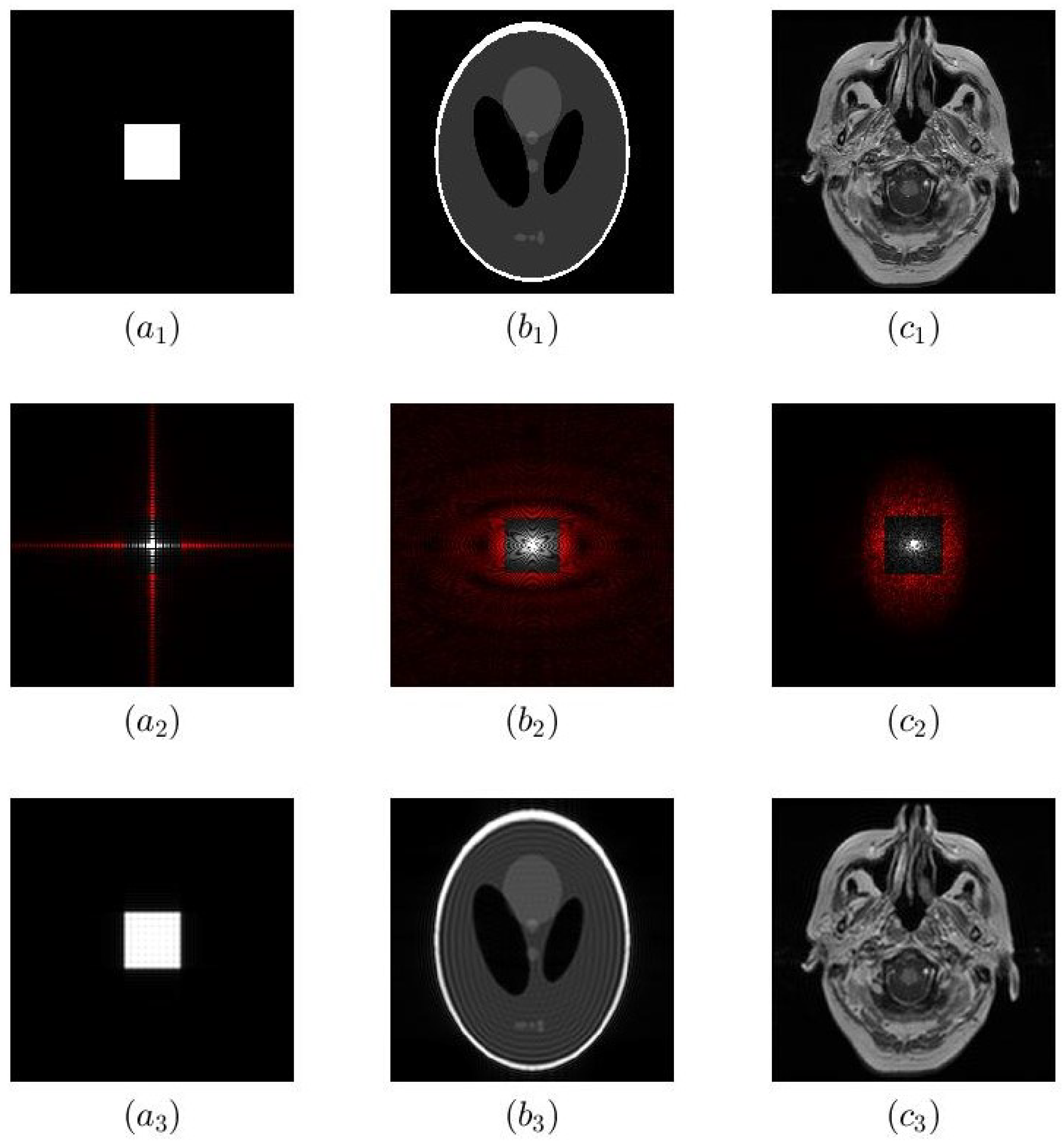
In this Section, we introduce the three test images, depicted in Figure 1. These range from the minimalist rectangle function, which provides a discontinuity and little else to confound analysis, to an example slice of an MRI for a more realistic test. This variety of test images makes our analysis more robust.
The first test image is a 400 × 400 image of a 2D rectangle function shown in Figure 1(). The central 200 × 200 pixels have value 1 and the remaining pixels are zeros. One of the advantages of this test image is that its Fourier transform can easily be calculated mathematically: it is a 2D sinc function. This means that we know the space and Fourier domain samples exactly, as opposed to other examples where we know only one domain exactly and must determine the other numerically at the cost of aliasing.
was sampled with 400 × 400 sampling points up to a cutoff frequency of 10,000 lines/mm in both x and y. The spectrum is truncated (in Figure 1(), truncation of 80% of Fourier coefficients is shown) and inverse Fourier transformed. The resulting image (Figure 1()) exhibits Gibbs ringing and can be compared with sampled at 20,000 lines/mm.
The second test image is shown in Figure 1() is a 400 × 400 Shepp–Logan phantom. It was developed as a test image for MRI reconstruction algorithms, resembling an MRI head section, and is a widely used test image in Gibbs ringing reduction studies in MRI [6,9,14]. The Fourier coefficients can be approximated by discrete Fourier transform of the phantom. We know the ground truth in the space domain, but do not know the Fourier domain samples exactly.
Finally, the third test image is a 512 × 512 pixel MRI slice obtained from the Brain Tumor Progression dataset [21] of The Cancer Imaging Archive [22]. We will refer to this as MR image. It is shown in Figure 1(). As before, we can use a discrete Fourier transform of the image to estimate the Fourier coefficients but, as with the Shepp–Logan phantom, we have a reduced reference. There is a small difference: the phantom is defined in the space domain, whereas the MR image was reconstructed from Fourier samples in the first place.
These three test images have increasing complexity: the rectangle function is a highly simplified test image; the phantom has edges that are not aligned with the x or y axis, which are not straight and which overlap; and the MRI is a real image with intricate details which lacks such clearly defined edges. We also have different knowledge about the ground truth of each image.
For all three images, we introduce ringing the same way. In the plots up to Figure 7, the central 20% of Fourier data remained on both the x and y axis. The magnitude of the Fourier data is shown in Figure 1(–). Fourier coefficients that are highlighted in red are set to zero. Adjusting the fraction of coefficients which are set to zero allows us to control the amount of ringing but maintain the number of samples to simplify comparisons. Figure 1(–) show the Fourier reconstruction based on the Fourier coefficients after truncation in the Fourier domain. There is visible ringing showing around the edges in all three images.
3. Metrics
Many previous studies that propose a novel reconstruction algorithm or post-processing method evaluate the outcomes qualitatively. Objective image quality metrics are desirable to facilitate automation of this assessment in order to facilitate the development of machine learning techniques and to eliminate inter- and intra-observer variation. In [17], we surveyed the literature on Gibbs ringing for MRI and found 12 metrics (e.g., PSNR, RMSE, entropy) that had been used in the past for assessing the quality of ringing reduction methods. We tested these twelve metrics to assess if they could pass a simple test: given a test image with ringing and a Gaussian filter of adjustable variance , could they identify which value of resulted in the best outcome. Large values of will blur the image less, but also will reduce ringing less. Small values of will suppress the ringing more, but will introduce more blurring. ’Best’, in this case, means that the ringing is suppressed and the blurring from the filter is not excessive. A suitable metric must exhibit a global minimum or maximum in this situation. We were forced to conclude that none of the 12 metrics were suitable for this problem.
We proposed a new full reference metric for evaluating Gibbs ringing suppression results called . We did not compare the inflection point of the curve with human perception of the image quality. We investigate the effect of varying in Section 5.
SSIM is known to be correlated with human perception. In this paper, we make the comparison between and SSIM. We also test SSIM as a potential full reference metric for ringing reduction. The definition of structural similarity index of two images, x and y, can be found in Equation (12) in [23].
The structural similarity ranges from 0 to 1. When the two images are identical, the value of SSIM is equal to one. The SSIM evaluates luminance, contrast and structure at the same time. SSIM is a commonly used metric for various fields. In our problem, we define y as the reconstructed image and x as the targeted ground truth. SSIM was used as a metric for Gibbs ringing measurement mostly in machine learning papers [12,14,15].
We evaluate SSIM for quantifying Gibbs ringing suppression in Section 3.1. Because SSIM is known to be correlated with human perception, we then use it as a benchmark when we investigate the effect of varying in Section 5.
It has been suggested that “For image quality assessment, it is useful to apply the SSIM index locally rather than globally” [23], which is one reason we investigate regions of interest in Section 4. However, the papers that utilized SSIM for evaluating Gibbs suppression all used it globally on the entire reconstructed image rather than on the region of interest with ringing artefacts. Therefore, we investigate MS-SSIM as a potential metric for evaluating Gibbs ringing suppression.
MS-SSIM was first proposed in [24]. The definition of MS-SSIM between image x and y can be found in Equation (7) in [24]. MS-SSIM is more flexible than SSIM because it has the ability to incorporate the variations of image resolution and viewing conditions. In this paper, the number of scales for MS-SSIM is five. The weights for each scale are 0.0545, 0.2442, 0.4026, 0.2442 and 0.0545. The weights follow a Gaussian distribution because human visual sensitivity peaks at middle frequencies and decreases in both directions.
MAE, also known as the loss, is a loss function used in linear regression models and is a useful measure widely used in model evaluations. MAE can be defined as
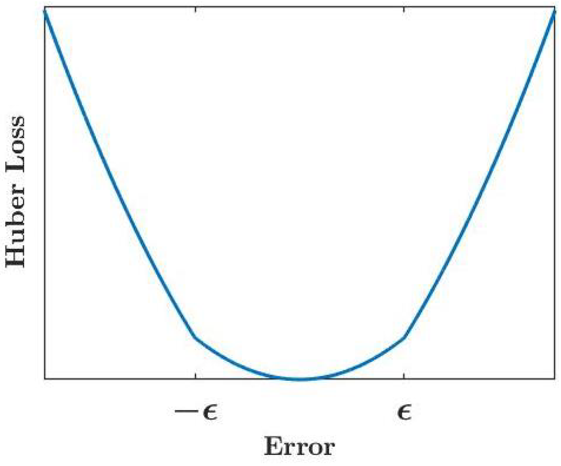
As we noted, works by counting the pixels with error above a certain threshold. Huber loss [25] is a loss function used in robust regression commonly used in statistics and machine learning. The Huber loss combines the strengths of MAE and MSE by balancing the MSE and MAE together. There is a parameter for Huber loss called the transition point. Huber loss can be defined as:
where is the transition point where the loss changes from a quadratic function to a linear function. represents the division between small errors we can tolerate and larger errors we wish to suppress. The transfer function of Huber loss is shown in Figure 2. When , Huber loss is also known as smooth loss. The definition used above is identically 0 when , so we replace that definition in the limiting case with MAE.
We evaluate Huber loss for quantifying Gibbs ringing suppression in Section 3.1 and investigate the effect of varying in Section 5.
Entropy of the reconstructed image was tested in [17], based on its use in [18,19], and proved unsatisfactory. However, in preparing this work, we have discovered that the definition of entropy in those papers is incorrect, using the pixel values of the reconstruction image in place of the normalized histogram of the reconstruction. We therefore test the correct definition of entropy in this paper.
where p contains the normalized histogram counts.
There are other metrics that were used in Gibbs ringing removal studies before, namely peak signal-to-noise ratio (PSNR) [12,14,15,18,19], mean squared error (MSE) [12,18], variance [19], variance of error [18], maximum error [26], signal-to-noise ratio (SNR) [27], energy [19], correlation [11,19], high frequency error norm (HFEN) [14], power spectral ratio (PSR) [13] and edge preservation index (EPI). It has been demonstrated that these metrics do not consistently find the balance between blurring and Gibbs ringing reduction in [17]. However, we also test those metrics in Section 4 to see if they show more promise when applied to a region of interest. PSR shows some interesting behaviour, so we additionally define it here.
3.1. Metrics Comparison Results
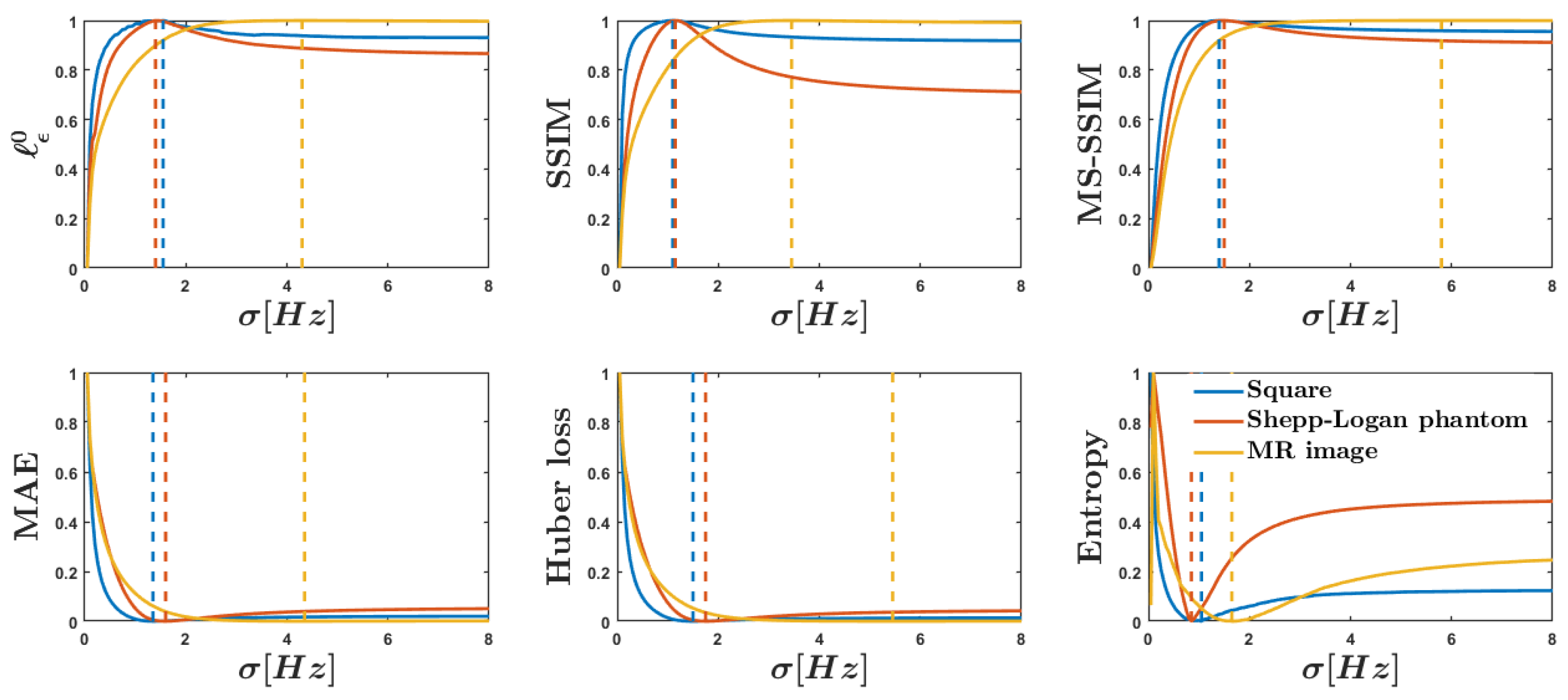
In this Section, we evaluate , SSIM, MS-SSIM, MAE, Huber loss and entropy for our problem. We compare the metrics using a series of filtered Fourier reconstruction results generated by Gaussian filters. Gaussian filters change the degree of filtering based on the single parameter that affects the cut-off frequency.
Figure 3 shows the evaluation of different Gaussian filters using , SSIM, MS-SSIM, MAE, Huber loss and entropy, all normalized to the range 0 to 1. The value of used for and Huber loss was , which is the order of magnitude of the median error of the Fourier reconstruction. It can be seen from the figure that all six metrics show peaks or nadirs for all three test images. We can see that for the phantoms the six metrics suggest comparable settings while, for the MRI, and MAE are the two that most closely agree with SSIM. and Huber loss could be further tuned to better fit human perception of ringing by adjusting . We note that MS-SSIM suggests more lenient filtering in comparison with the results of SSIM. We will discuss that further in Section 5.
We conclude that all six of these metrics are candidates for assessing Gibbs ringing quantitatively.
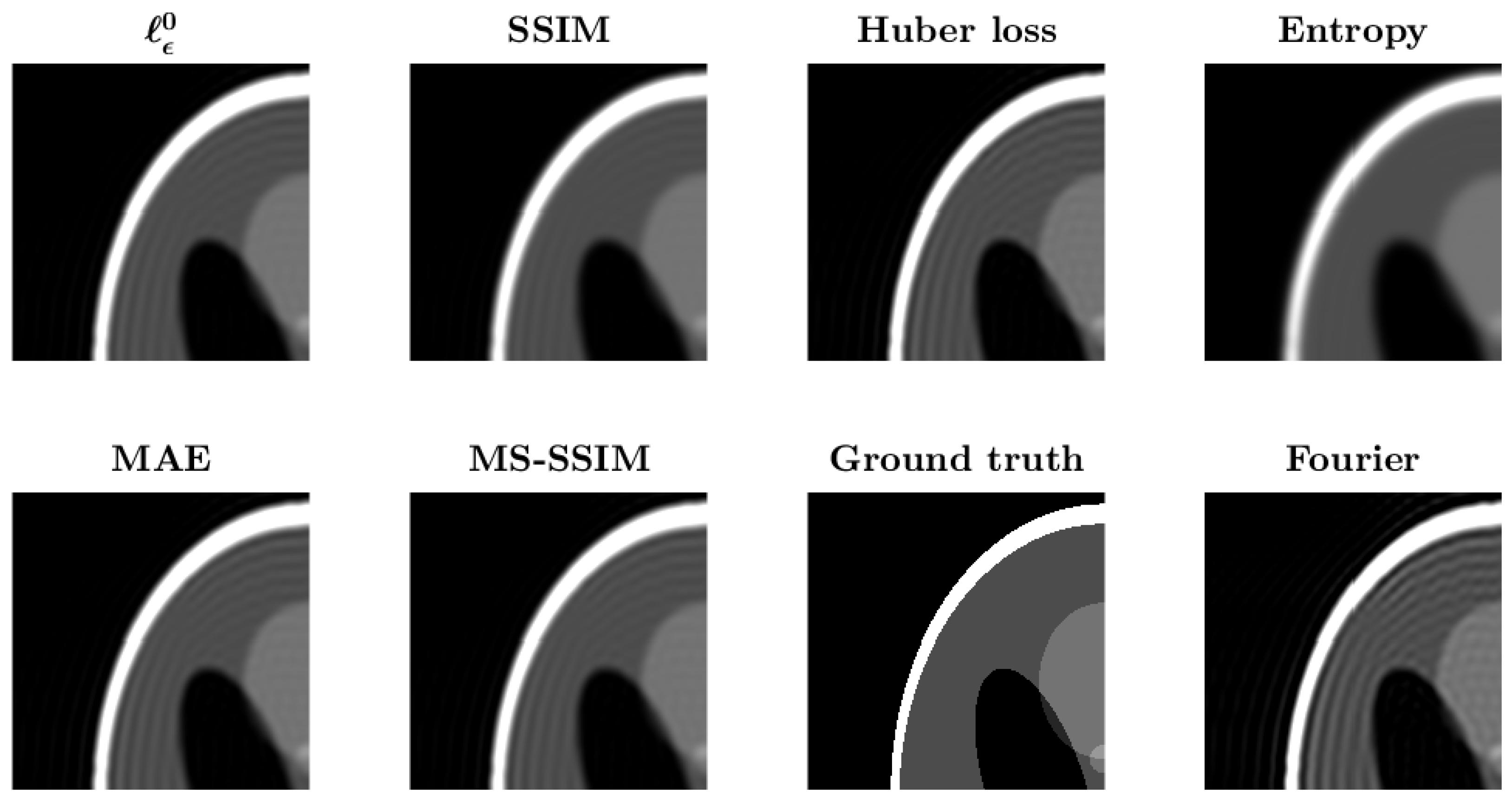
In Figure 4, we present the optimal reconstructions of the Shepp–Logan phantom from the different metrics. For reference, we also show the ground truth without ringing and the Fourier reconstruction with added ringing. It can be seen from the figure that , Huber loss and MAE agree with the result of SSIM. The suggestion of entropy is blurry, which suggests too much filtering, whereas the results of MS-SSIM does not reduce ringing as much as possible.
4. Region of Interest
As we noted earlier, it has been suggested that “For image quality assessment, it is useful to apply the SSIM index locally rather than globally” [23]. Gibbs ringing is the most severe around discontinuities. We therefore speculate that applying metrics to a limited region near edges could enhance their sensitivity to ringing, which could overcome the problems we identified previously. This approach of identifying the region of interest (RoI) means that the spatial information of each pixel is taken into account. Will the performances of the metrics increase with the use of an RoI? In this section, we propose a method to identify the RoI based on high pass filtering, binarization, and erosion and dilation. We then evaluate 16 metrics on this region of the test image.
The steps we used to calculate the RoI are shown in Figure 5. For space reasons, we limit the example to the phantom, though we have also tested it on the other two test images. It is assumed that the ground truth is known. In practical situations, the RoI might have to be estimated from a Fourier reconstruction. Figure 5a shows the original Shepp–Logan phantom (i.e., without ringing).
- The image is normalized to have maximum value 1.
- A Laplacian of Gaussian (LoG) filter with rotational symmetry, kernel size of 4 × 4 and standard deviation = 0.2.
- The image is then binarized with threshold 0.5.
- Image erosion is applied with a flat morphological structuring element object of size 3 × 3.
- Image dilation is applied with a flat morphological structuring element object of size 20 × 20.
Steps 1–3 highlight the regions where intensity changes rapidly. Figure 5b shows the result after passing the original image through the LoG filter and binarization. It can be seen that the locations of edges were extracted from the original image. Step 4 is shown in Figure 5c. Image erosion removes small objects. Step 5 then dilates the resulting edges to go from a representation of the edges to one of the region around edges. The final results are shown in Figure 5d. The parameters of the image erosion and dilation were chosen empirically.
Figure 6 shows the 200th row of the Shepp–Logan phantom (with ringing) and the corresponding RoI. The red line shows the RoI and the blue line shows the remainder of the signal. It is evident that the RoI includes the parts of the image where the ringing is strongest.
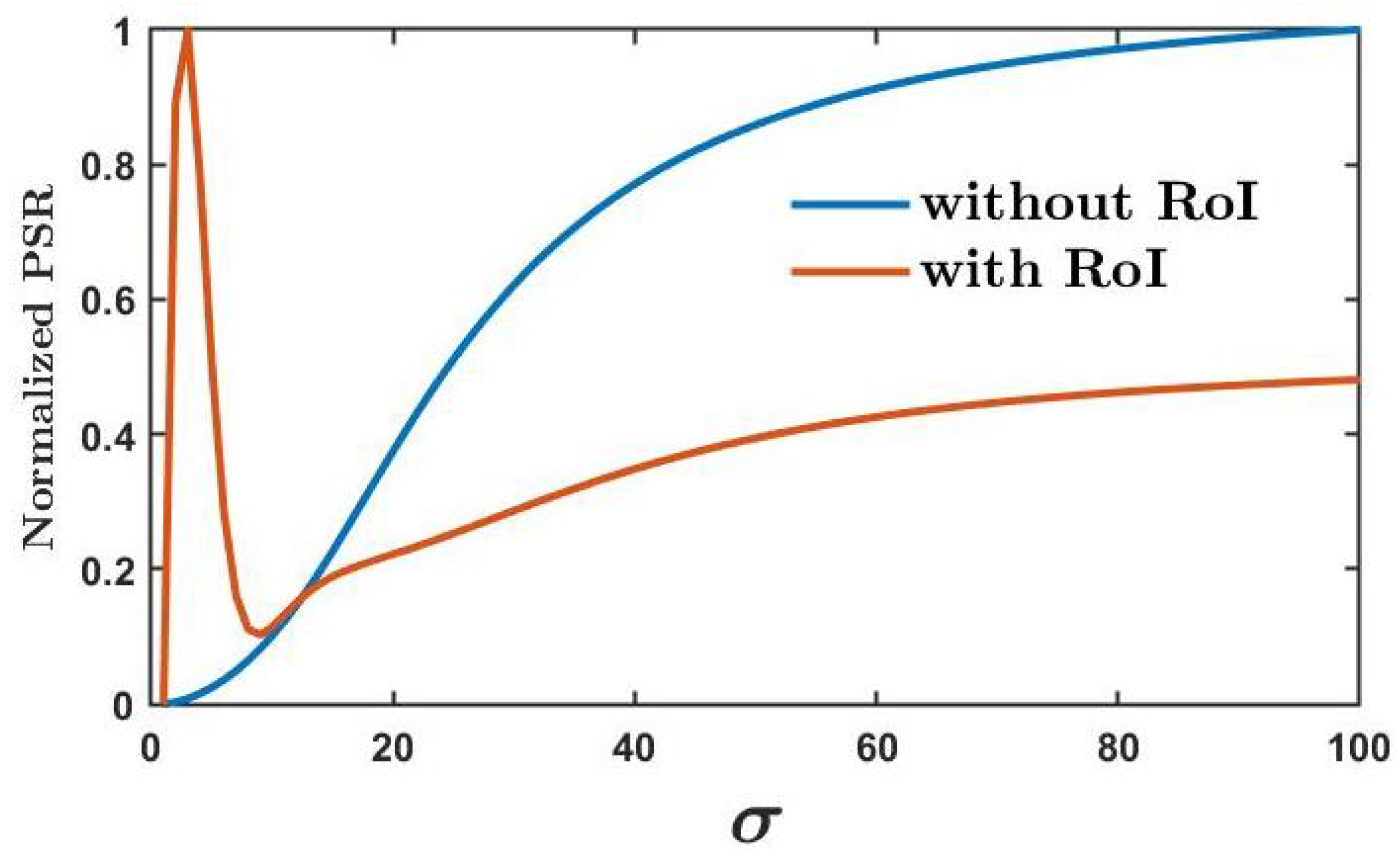
Next, we apply , SSIM, MS-SSIM, Huber loss, MAE, entropy and all 12 metrics discussed in [17] to the RoI. Unfortunately, almost all of the metrics show no significant changes. , SSIM, Huber loss, MAE and entropy show peaks or nadirs for similar values of when applied to the RoI or to the whole image. All other metrics but one show no peak with or without RoI. The exception is PSR.
Figure 7 shows the behaviour of PSR with and without the RoI. It can be seen that, applied to the whole image, PSR shows a monotonic upward trend. Applied to the RoI, PSR shows a peak and a local minimum. The peak is for very small , which would introduce an unreasonable amount of blurring. Taken in isolation, the local minimum is more potentially useful. However, given there are several other metrics which show useful global maxima and minima, this metric remains of limited utility.
We have demonstrated that most Gibbs metrics do not benefit from being applied to an RoI rather than the whole image.
5. The Effect of Varying the Threshold, , on and Huber Loss
In this section, we focus on the significance of the parameter . For two of the metrics discussed in Section 3, namely and Huber loss, is the boundary between small errors—which can be either completely ignored () or diminished by squaring (Huber loss)—and larger errors which contribute to the measurement of error. As ringing is an oscillating artefact with zero mean, we have speculated that any error metric that weights larger errors more highly than lower ones may also be able to distinguish ringing from other errors such as blur. Our investigation in Section 3.1 demonstrates that this is indeed the case for those two metrics. In our previous work, when we proposed as a metric in Gibbs suppression, we chose to use the median error of the Fourier reconstruction as a somewhat arbitrary but easily obtained value for , which seemed to work satisfactorily. We now wish to set that parameter based on something more evidence-based. Ideally, that evidence base would have some relationship to human perception. We note the concept of “just noticeable difference” (JND) [28]. The JND is “the minimum amount by which a stimulus intensity must be changed relative to a background intensity in order to produce a noticeable variation in sensory experience” [29]. Such perceptual thresholds depend on ambient light, the display screen and the idiosyncrasies of the vision of the observer, frustrating the desire for a single definitive answer. With that caveat, we now wish to address the question: how can we choose ?
Our standard problem to evaluate a metric, as depicted in, e.g., Figure 3, is truncate a test signal or image in the Fourier domain, use Gaussian filters of different variance, , to suppress the ringing in the Fourier reconstructed image and plot the metric as a function of . The for which the peak (or minimum) value of the metric is observed is then taken to characterize a ’best’ filter according to that metric. We have observed that both -dependent metrics exhibit a peak for many possible values of . However, the location of this peak varies with .
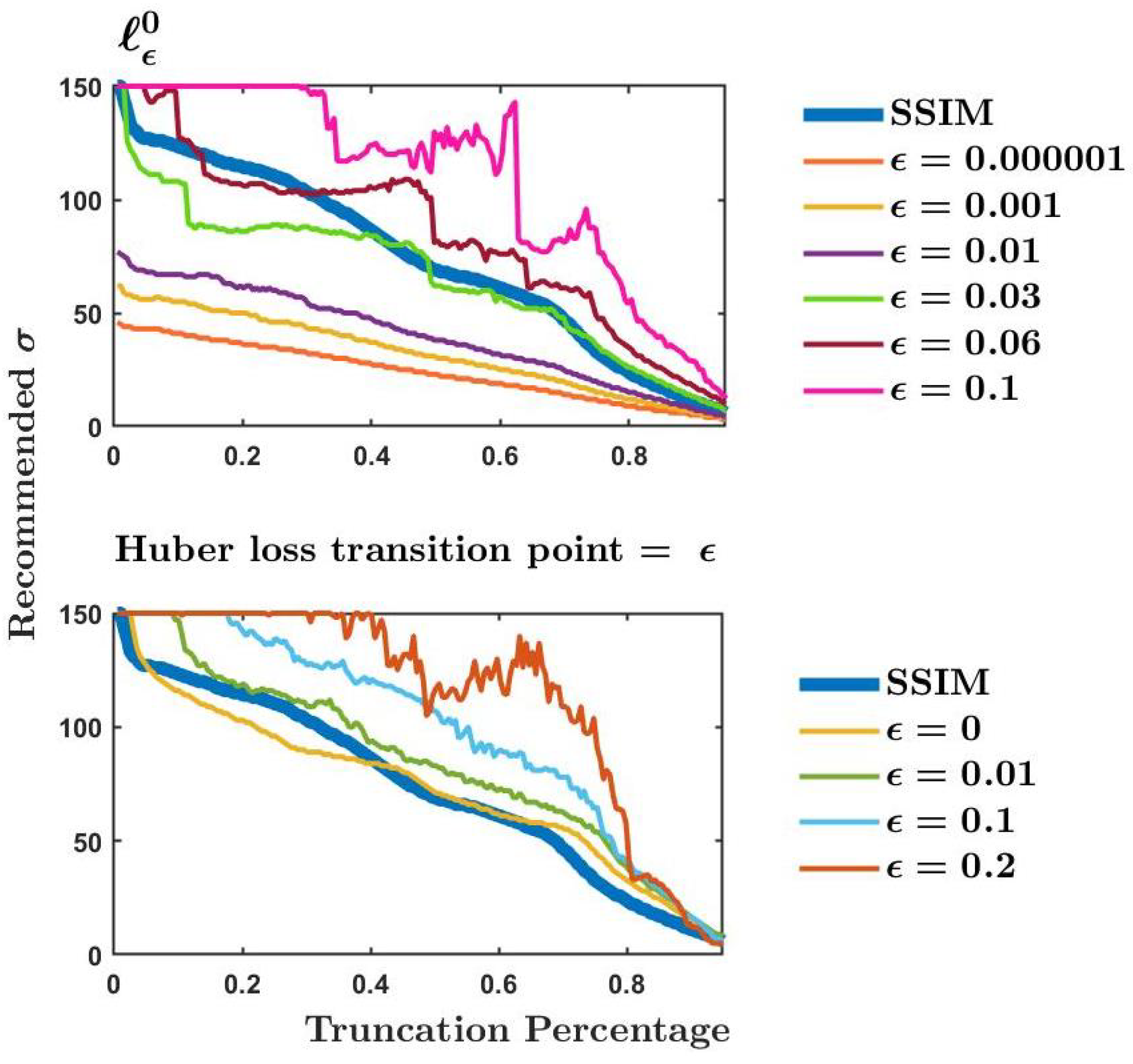
We can obtain a continuum of test images by treating the fraction of the Fourier coefficients that are set to zero as a variable. This ’truncation percentage’ was fixed for Figure 3 at 80% (i.e., only the central 20% of coefficients are retained). In Figure 8, we plot the ’best’ according to our two -dependent metrics as a function of truncation percentage for a variety of values of . We also plot the ’best’ according to SSIM as a benchmark against which to compare the other metrics. This, it must be acknowledged, is a somewhat arbitrary benchmark, but (a) it has been shown to be a useful metric for this problem and (b) it has been shown to correlate with human perception. In the absence of a large user evaluation study, we are forced to rely on a proxy metric of this kind. We do not claim that the results are therefore a definitive determination of the best but rather they are indicative of the general trends associated with varying that parameter. We also note that our test images are normalized to have maximum values of 1. The results in Figure 8 are for the Shepp–Logan phantom only in order to simplify the presentation of results, but we have also performed these simulations for the other two test images described in Section 2 with similar results.
First let us consider , in the upper plot of Figure 8. We observe near-linear plots for small , small here meaning . and approximately bracket the SSIM curve, meaning that the maximal agreement between and SSIM is in this region of . Larger values of result in an erratic plot, which does not inspire confidence in the recommendation of the ’best’ .
Next, we consider Huber loss, in the lower plot of Figure 8. For the case, we use the norm. We observe that small values of () cause Huber loss to track the SSIM curve rather well. The SSIM curve almost acts as a limiting case of Huber loss: no value of causes Huber loss to recommend significantly lower than SSIM. This means that Huber loss is biased towards less aggressive filtering, favouring less blur over better ringing suppression.
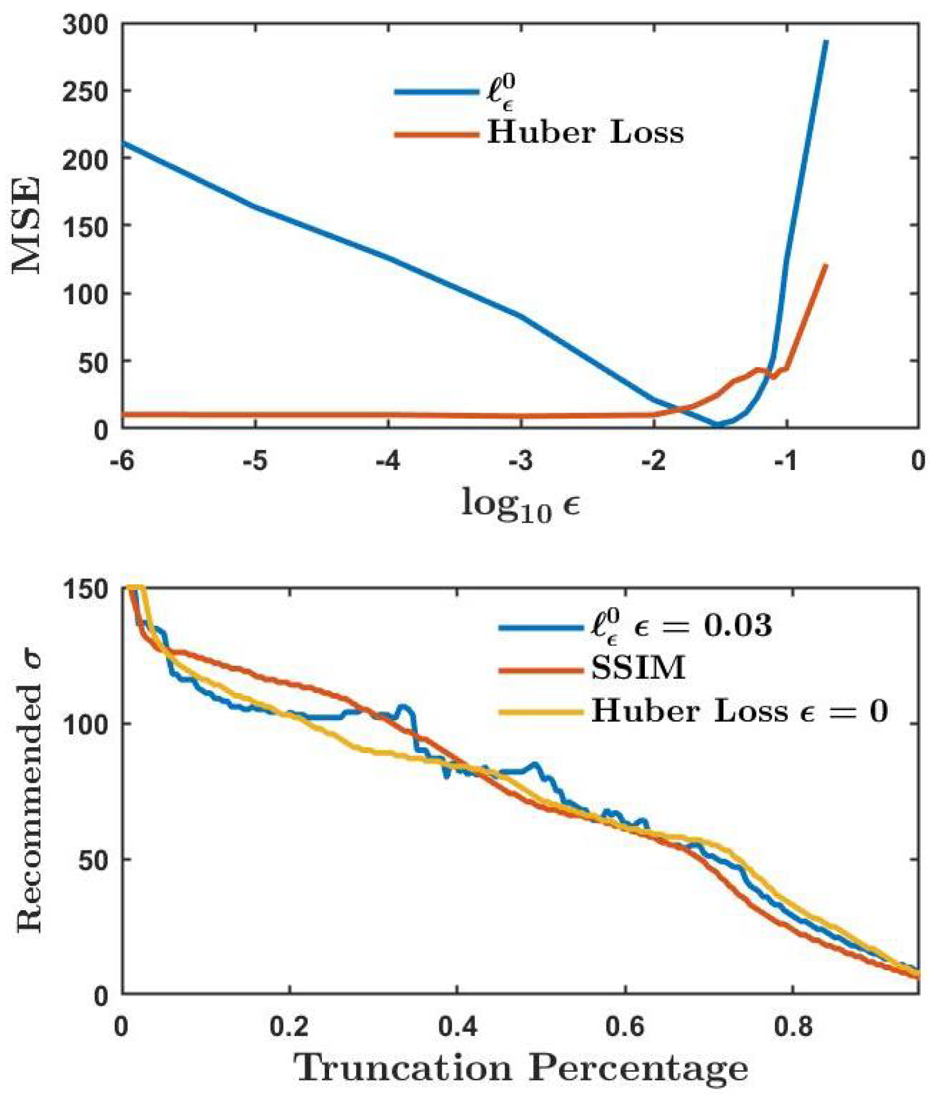
Next, we consider the upper plot in Figure 9. This shows the mean squared error between the curves in Figure 8 and the SSIM curve as a function of (which is log-scaled for clarity because of the distribution of values tested). The blue curve depicts the MSE between the recommendations of and of SSIM. It suggests that, when , the MSE between and SSIM is minimized. The red curve shows the MSE between Huber loss and SSIM. It shows that, when , the MSE between Huber loss and SSIM is minimized. With the caveats noted earlier, values close to 0.03 and 0 are therefore the optimal values of for and Huber loss, respectively, given test images normalized to a peak value of 1. Both metrics correlate well with SSIM for these choices of and therefore presumably with human perception. This is depicted in the lower plot of Figure 9.
We have shown the significance of , the threshold used in and in Huber loss. We have determined optimal values of these thresholds.
6. Conclusions
Gibbs ringing is an imaging problem that could be suppressed through both traditional and learning approaches. These methods, including the combined methods, all intend to provide images with less ringing. In the literature, the merits of Gibbs suppression algorithms have been assessed with a mixture of qualitative and a variety of quantitative metrics. In a recent paper, the authors surveyed the quantitative metrics used in previous reports of novel Gibbs suppression algorithms and found them wanting [17]. However, it is only with good, consistent and convenient quantitative metrics can we provide critical comparisons between traditional and learning methods.
We proposed the metric for this purpose in our previous paper [17]. In this paper, we have extended our analysis to consider SSIM, MS-SSIM, Huber loss, MAE and a corrected definition of entropy. We have shown that those metrics join in passing our test: given a variety of Gaussian filters, they can identify a ’best’ one which trades off ringing suppression against blur. This is a necessary requirement of a good quantitative metric, though we do not claim it is a sufficient one.
We had good reasons to investigate a region of interest limited to parts of the image close to edges as a means of enhancing or rehabilitating the 17 metrics we have investigated. We proposed an algorithm for finding such a region, but have found the approach had limited effect on the metrics.
Finally, two of the metrics depended on an error threshold. We have investigated the effects of varying that threshold. Our results show that Huber loss is optimized by minimizing the threshold; in the limit, it becomes the norm. For this minimal threshold, it provides good agreement with the SSIM. We have also seen that has good agreement with SSIM for a suitable choice of . For smaller values of , it tolerates less error and so recommends more aggressive filters. It does so quite consistently: a small increase in Fourier domain truncation results in a small increase in the recommended filtering. For larger values of , this consistency is lost and the metric may not be as reliable as we might like. Thus, larger values of the threshold are recommended against.
The work in this paper will help provide a foundation of evidence-led best practice in the comparison of Gibbs suppression algorithms, both traditional and learning approaches included.
Author Contributions
Conceptualization, Y.W. and J.J.H.; methodology, J.J.H.; software, Y.W.; validation, Y.W.; formal analysis, Y.W. and J.J.H.; investigation, Y.W.; resources, J.J.H.; data curation, Y.W.; writing—original draft preparation, Y.W. and J.J.H.; writing—review and editing, Y.W. and J.J.H.; visualization, Y.W. and J.J.H.; supervision, J.J.H.; project administration, J.J.H.; funding acquisition, Y.W. and J.J.H. All authors have read and agreed to the published version of the manuscript.
Funding
This research was funded by GliMR EU COST Action grant number CA18206. Yue Wang was funded by Irish Research Council Government of Ireland Postgraduate Scholarship.
Institutional Review Board Statement
Not applicable.
Informed Consent Statement
Not applicable.
Data Availability Statement
Not applicable.
Acknowledgments
The authors would like to thank University College Dublin for support. The authors would like to thank our colleague Cliodhna Gartland for constructive conversations in relation to this work.
Conflicts of Interest
The authors declare no conflict of interest.
Abbreviations
The following abbreviations are used in this manuscript:
| MRI | Magnetic resonance imaging |
| CNN | Convolutional neural network |
| SSIM | Structural similarity index |
| MS-SSIM | Multi-scale SSIM index |
| MAE | Mean absolute error |
| PSNR | Peak signal-to-noise ratio |
| SNR | Signal-to-noise ratio |
| RMSE | Root mean square error |
| EPI | Edge preservation index |
| MSE | Mean square error |
| HFEN | High frequency error norm |
| PSR | Power spectral ratio |
| RoI | Region of interest |
| LoG | Laplacian of Gaussian |
| JND | Just noticeable difference |
References
- Sotthivirat, S.; Fessler, J.A. Penalized-likelihood image reconstruction for digital holography. J. Opt. Soc. Am. A 2004, 21, 737–750. [Google Scholar] [CrossRef]
- León-Rodríguez, M.; Cordero, R.R.; Rayas, J.A.; Martínez-García, A.; Martínez-Gonzalez, A.; Labbe, F.; Téllez-Quiñones, A.; Flores-Muñoz, V. Reduction of the ringing effect in off-axis digital holography reconstruction from two reconstruction distances based on Talbot effect. Opt. Eng. 2015, 54, 104110. [Google Scholar] [CrossRef]
- Sung, Y.; Dasari, R.R. Deterministic regularization of three-dimensional optical diffraction tomography. J. Opt. Soc. Am. A 2011, 28, 1554–1561. [Google Scholar] [CrossRef]
- Godden, T.; Muñiz-Piniella, A.; Claverley, J.; Yacoot, A.; Humphry, M. Phase calibration target for quantitative phase imaging with ptychography. Opt. Express 2016, 24, 7679–7692. [Google Scholar] [CrossRef]
- Shimobaba, T.; Hoshi, I.; Shiomi, H.; Wang, F.; Hara, T.; Kakue, T.; Ito, T. Mitigating ringing artifacts in diffraction calculations using average subtractions. Appl. Opt. 2021, 60, 6393–6399. [Google Scholar] [CrossRef]
- Archibald, R.; Gelb, A. A method to reduce the Gibbs ringing artifact in MRI scans while keeping tissue boundary integrity. IEEE Trans. Med. Imaging 2002, 21, 305–319. [Google Scholar] [CrossRef]
- Gottlieb, D.; Shu, C.W.; Solomonoff, A.; Vandeven, H. On the Gibbs phenomenon I: Recovering exponential accuracy from the Fourier partial sum of a nonperiodic analytic function. J. Comput. Appl. Math. 1992, 43, 81–98. [Google Scholar] [CrossRef]
- Gottlieb, D.; Shu, C.W. On the Gibbs phenomenon and its resolution. SIAM Rev. 1997, 39, 644–668. [Google Scholar] [CrossRef]
- Gelb, A. A hybrid approach to spectral reconstruction of piecewise smooth functions. J. Sci. Comput. 2000, 15, 293–322. [Google Scholar] [CrossRef]
- Ferreira, P.; Gatehouse, P.; Kellman, P.; Bucciarelli-Ducci, C.; Firmin, D. Variability of myocardial perfusion dark rim Gibbs artifacts due to sub-pixel shifts. J. Cardiovasc. Magn. Reson. 2009, 11, 1–10. [Google Scholar] [CrossRef] [Green Version]
- Kellner, E.; Dhital, B.; Kiselev, V.G.; Reisert, M. Gibbs-ringing artifact removal based on local subvoxel-shifts. Magn. Reson. Med. 2016, 76, 1574–1581. [Google Scholar] [CrossRef]
- Zhang, Q.; Ruan, G.; Yang, W.; Liu, Y.; Zhao, K.; Feng, Q.; Chen, W.; Wu, E.X.; Feng, Y. MRI Gibbs-ringing artifact reduction by means of machine learning using convolutional neural networks. Magn. Reson. Med. 2019, 82, 2133–2145. [Google Scholar] [CrossRef]
- Muckley, M.J.; Ades-Aron, B.; Papaioannou, A.; Lemberskiy, G.; Solomon, E.; Lui, Y.W.; Sodickson, D.K.; Fieremans, E.; Novikov, D.S.; Knoll, F. Training a neural network for Gibbs and noise removal in diffusion MRI. Magn. Reson. Med. 2021, 85, 413–428. [Google Scholar] [CrossRef]
- Wang, Y.; Song, Y.; Xie, H.; Li, W.; Hu, B.; Yang, G. Reduction of Gibbs artifacts in magnetic resonance imaging based on Convolutional Neural Network. In Proceedings of the 2017 IEEE 10th International Congress on Image and Signal Processing, Biomedical Engineering and Informatics (CISP-BMEI), Shanghai, China, 14–16 October 2017; pp. 1–5. [Google Scholar]
- Zhao, X.; Zhang, H.; Zhou, Y.; Bian, W.; Zhang, T.; Zou, X. Gibbs-ringing artifact suppression with knowledge transfer from natural images to MR images. Multimed. Tools Appl. 2020, 79, 33711–33733. [Google Scholar] [CrossRef]
- Penkin, M.; Krylov, A.S.; Khvostikov, A.V. Hybrid Method for Gibbs-Ringing Artifact Suppression in Magnetic Resonance Images. Program. Comput. Softw. 2021, 47, 207–214. [Google Scholar] [CrossRef]
- Wang, Y.; Healy, J.J. Automated filter selection for suppression of Gibbs ringing artefacts in MRI. Magn. Reson. Imaging 2022, 93, 3–10. [Google Scholar] [CrossRef]
- Roberts, B.; Wan, M.; Kelly, S.P.; Healy, J.J. Quantitative comparison of Gegenbauer, filtered Fourier, and Fourier reconstruction for MRI. In Proceedings of the Multimodal Biomedical Imaging XV—International Society for Optics and Photonics, San Francisco, CA, USA, 1–6 February 2020; Volume 11232, p. 112320L. [Google Scholar]
- Seetha, J.; Raja, S.S. Denoising of MRI images using filtering methods. In Proceedings of the 2016 IEEE International Conference on Wireless Communications, Signal Processing and Networking (WiSPNET), Chennai, India, 23–25 March 2016; pp. 765–769. [Google Scholar]
- Tian, C.; Xu, Y.; Li, Z.; Zuo, W.; Fei, L.; Liu, H. Attention-guided CNN for image denoising. Neural Netw. 2020, 124, 117–129. [Google Scholar] [CrossRef]
- Schmainda, K.; Prah, M. Data from Brain-Tumor-Progression. The Cancer Imaging Archive. 2018. Available online: https://wiki.cancerimagingarchive.net/display/Public/Brain-Tumor-Progression (accessed on 13 December 2022).
- Clark, K.; Vendt, B.; Smith, K.; Freymann, J.; Kirby, J.; Koppel, P.; Moore, S.; Phillips, S.; Maffitt, D.; Pringle, M.; et al. The Cancer Imaging Archive (TCIA): Maintaining and operating a public information repository. J. Digit. Imaging 2013, 26, 1045–1057. [Google Scholar] [CrossRef]
- Wang, Z.; Bovik, A.C.; Sheikh, H.R.; Simoncelli, E.P. Image quality assessment: From error visibility to structural similarity. IEEE Trans. Image Process. 2004, 13, 600–612. [Google Scholar] [CrossRef]
- Wang, Z.; Simoncelli, E.P.; Bovik, A.C. Multiscale structural similarity for image quality assessment. In Proceedings of the IEEE Thrity-Seventh Asilomar Conference on Signals, Systems & Computers, Pacific Grove, CA, USA, 9–12 November 2003; Volume 2, pp. 1398–1402. [Google Scholar]
- Huber, P.J. Robust estimation of a location parameter. In Breakthroughs in Statistics; Springer: New York, NY, USA, 1992; pp. 492–518. [Google Scholar]
- Di Bella, E.; Parker, D.; Sinusas, A. On the dark rim artifact in dynamic contrast-enhanced MRI myocardial perfusion studies. Magn. Reson. Med. Off. J. Int. Soc. Magn. Reson. Med. 2005, 54, 1295–1299. [Google Scholar] [CrossRef] [PubMed] [Green Version]
- Parker, D.L.; Gullberg, G.T.; Frederick, P.R. Gibbs artifact removal in magnetic resonance imaging. Med. Phys. 1987, 14, 640–645. [Google Scholar] [CrossRef] [PubMed]
- Jayant, N.; Johnston, J.; Safranek, R. Signal compression based on models of human perception. Proc. IEEE 1993, 81, 1385–1422. [Google Scholar] [CrossRef]
- Ferzli, R.; Karam, L.J. A no-reference objective image sharpness metric based on the notion of just noticeable blur (JNB). IEEE Trans. Image Process. 2009, 18, 717–728. [Google Scholar] [CrossRef] [PubMed]
Figure 1.
The three test images before and after introducing ringing. () Original 400 × 400 numerically simulated square. () Original 400 × 400 Shepp–Logan phantom. () Original 512 × 512 MR image. (–) Spectra of (–). Fourier coefficients highlighted in red are set to zero, simulating zero padding of a reduced number of measured Fourier coefficients. (–) Fourier reconstruction using (–) showing visible ringing.

Figure 2.
The transfer function of Huber loss. is the transition point.

Figure 3.
Evaluation of different Gaussian filters using , SSIM, MS-SSIM, MAE, Huber loss and entropy. In all sections of the figure, we plot the results for the ideal square test image (blue), the Shepp–Logan phantom (red) and an MR head section (yellow). The dotted vertical lines of the same colour indicate a peak/nadir of the three metrics.

Figure 4.
The optimal reconstructions of the Shepp–Logan phantom from the different metrics. For reference, we also show the ground truth without ringing and the Fourier reconstruction with added ringing.
Figure 4.
The optimal reconstructions of the Shepp–Logan phantom from the different metrics. For reference, we also show the ground truth without ringing and the Fourier reconstruction with added ringing.

Figure 5.
The process of determining the RoI. (a) Original Shepp–Logan phantom. (b) After LoG filter and binarization. (c) Image erosion of (b). (d) Image dilation of (c).
Figure 5.
The process of determining the RoI. (a) Original Shepp–Logan phantom. (b) After LoG filter and binarization. (c) Image erosion of (b). (d) Image dilation of (c).

Figure 6.
1D slice of the Shepp–Logan phantom with ringing. The RoI is in red. The excluded regions are in blue.
Figure 6.
1D slice of the Shepp–Logan phantom with ringing. The RoI is in red. The excluded regions are in blue.

Figure 7.
The behaviours of PSR applied to the whole image (blue) and to the RoI (red). Applied to the RoI, the metric shows a local maximum and a local minimum.
Figure 7.
The behaviours of PSR applied to the whole image (blue) and to the RoI (red). Applied to the RoI, the metric shows a local maximum and a local minimum.

Figure 8.
(top) SSIM (thick blue) and for various values of . (bottom) SSIM (thick blue) and Huber loss for various values of .
Figure 8.
(top) SSIM (thick blue) and for various values of . (bottom) SSIM (thick blue) and Huber loss for various values of .

Figure 9.
(top) Mean squared error as a function of between SSIM and (blue), and between SSIM and Huber loss (red). Best values of are identified by the minima. (bottom) Best for the Gaussian filter as a function of truncation percentage, as recommended by the three metrics (using as identified above).

Disclaimer/Publisher’s Note: The statements, opinions and data contained in all publications are solely those of the individual author(s) and contributor(s) and not of MDPI and/or the editor(s). MDPI and/or the editor(s) disclaim responsibility for any injury to people or property resulting from any ideas, methods, instructions or products referred to in the content. |
© 2023 by the authors. Licensee MDPI, Basel, Switzerland. This article is an open access article distributed under the terms and conditions of the Creative Commons Attribution (CC BY) license (https://creativecommons.org/licenses/by/4.0/).
Share and Cite
MDPI and ACS Style
Wang, Y.; Healy, J.J. Image Quality Assessment for Gibbs Ringing Reduction. Algorithms 2023, 16, 96. https://doi.org/10.3390/a16020096
AMA Style
Wang Y, Healy JJ. Image Quality Assessment for Gibbs Ringing Reduction. Algorithms. 2023; 16(2):96. https://doi.org/10.3390/a16020096
Chicago/Turabian StyleWang, Yue, and John J. Healy. 2023. "Image Quality Assessment for Gibbs Ringing Reduction" Algorithms 16, no. 2: 96. https://doi.org/10.3390/a16020096
Note that from the first issue of 2016, this journal uses article numbers instead of page numbers. See further details here.