Article

A Constructive Heuristics and an Iterated Neighborhood Search Procedure to Solve the Cost-Balanced Path Problem

by
Daniela Ambrosino
*,†,
Carmine Cerrone
and
Anna Sciomachen
Department of Economics and Business Studies, University of Genoa, 16126 Genoa, Italy
*
Author to whom correspondence should be addressed.
These authors contributed equally to this work.
Algorithms 2022, 15(10), 364; https://doi.org/10.3390/a15100364
Submission received: 31 July 2022 / Revised: 24 September 2022 / Accepted: 27 September 2022 / Published: 29 September 2022

Abstract

:
This paper presents a new heuristic algorithm tailored to solve large instances of an NP-hard variant of the shortest path problem, denoted the cost-balanced path problem, recently proposed in the literature. The problem consists in finding the origin–destination path in a direct graph, having both negative and positive weights associated with the arcs, such that the total sum of the weights of the selected arcs is as close to zero as possible. At least to the authors’ knowledge, there are no solution algorithms for facing this problem. The proposed algorithm integrates a constructive procedure and an improvement procedure, and it is validated thanks to the implementation of an iterated neighborhood search procedure. The reported numerical experimentation shows that the proposed algorithm is computationally very efficient. In particular, the proposed algorithm is most suitable in the case of large instances where it is possible to prove the existence of a perfectly balanced path and thus the optimality of the solution by finding a good percentage of optimal solutions in negligible computational time.

1. Introduction

In many optimization problems arising in the decision science area, given a finite set E of elements having a vector cost c associated with them, the objective function is to find a feasible subset F E , such that the difference in value between the most costly and the least costly selected elements is minimized. Such problems are denoted as balanced optimization problems (BOPs). One of the first approaches to solve a BOP is presented in [1], where the authors consider the set E as an n × n assignment matrix, the cost c e as the value contained in a generic cell e of the assignment matrix, and the subset F the selected cells of the defined assignment, thus obtaining the balanced assignment problem. Successively, Ref. [2] introduced the minimum deviation problem, which minimizes the difference between the maximum and average weights in a solution. In the same paper, the authors proposed a general solution scheme also suitable for BOPs. Since then, numerous real-world applications have been defined and solved as BOPs, always with the goal of minimizing the deviation between the highest and lowest cost, or making the performance indices of interest as equal as possible. In the latter case, the most proposed applications in the literature as BOPs include, though are not limited to, production line operations in manufacturing systems (e.g., see [3,4,5,6] among others) and supply chain management [7,8]. Other BOPs were proposed in the class of flow and routing problems on networks, where the goal is to design either a single path or a subset of paths in which the arcs or nodes belonging to the solution have a homogeneous value of their relative weights, such as travel time, length, etc. (see [9,10,11], among others).
This paper deals with a variant of the Shortest Path Problem ( S P P ) that fits into the class of BOPs. This problem, recently introduced in the literature [12], is denoted Cost Balanced Path Problem ( C B P P ).
The C B P P is defined on a directed weighted graph G ( N , A ) , where N is the set of nodes and A is the set of directed arcs. For each arc ( i , j ) A there is a weight c i j R ; the weights represent either the increment (in case of positive weight) or the decrement (in case of negative weight) of the cost to balance along the path. The problem is to select in graph G a path p from an origin node o to a destination node d that minimizes the absolute value of the sum of the weights of path p. More formally, the objective function of the C B P P is given by:
M I N | c ( p ) | = | ( i , j ) p c i j |
In [12] the authors demonstrate that the C B P P , as many variants of the S P P [13], is NP-hard in its general form. Moreover, they demonstrate that, in the following two particular cases, the C B P P can be solved in polynomial time:
  • When all costs are non-negative or non-positive (i.e., c i j 0 or c i j 0 , ( i , j ) A ). In this case, the problem is equivalent to the S P P ;
  • When the cost of the arc is a function of the elevation difference of the two nodes associated with the arc.
The reader may observe that the objective function (1) imposes minimization of an always positive value. For this reason, zero is a lower bound for the CBPP. This implies that any solution with zero objective function value, coincident with the lower bound, will always be optimal. The C B P P can be used for modelling various real problems that require the decision-maker to choose a path in a graph from an origin node to a destination one balancing some elements. Among others, the problems of route design for automated guided vehicles, the vehicles’ loading in pick-up and delivery, and storage and retrieval problems in warehouses and yards deserve attention. Another interesting application of the CBPP concerns electric vehicles with limited battery levels, considering, for example, that maintaining a lithium battery at a charge value of about 80 % helps to extend its life. In this case, given a graph, the positive or negative values associated with arcs represent, respectively, energy consumption or recharging obtained on downhill roads or through charging stations. Identifying a path in this graph so that the car arrives at its destination with a similar level of charge as at the start would extend the average life of a battery.
In [12], the authors proposed a mixed-integer linear programming model for solving the C B P P and tested it by using different sets of random instances. Experimental tests on the model showed that the computation time of instances that do not have zero as the optimal solution is significantly higher. For these more complex instances, it is, therefore, necessary to develop heuristic algorithms. Unfortunately, at least to the authors’ knowledge, no solution approaches for the C B P P have been proposed in the literature. Instead, heuristic algorithms have been presented for some problems closely related to the C B P P .
One of the most relevant and similar problem to the C B P P is the cost-balanced Travelling Salesman Problem ( T S P ) introduced in [14], in which the main objective is to find a Hamiltonian cycle in a graph with total travel cost as close to zero as possible. In [15], the authors propose a variable neighborhood search algorithm, which is a local search with multiple neighborhood structures, to solve the cost-balanced T S P . The balanced T S P is widely described in [16], where an equitable distribution of resources is the main objective. The authors cited many balanced combinatorial optimization problems studied in the literature, and proposed four different heuristics, derived by the double-threshold algorithm and the bottleneck one, to solve the balanced T S P . To solve the same problem, in [17] an adaptive iterated local search is proposed with a perturbation and a random restart that can help in escaping local optimum. In [18], a multiple balanced TSP is analyzed to model and optimize the problems with multiple objectives (salesmen). The goal is to find m Hamiltonian cycles in a graph G by minimizing the difference between the highest edge cost and the smallest edge cost in the tours.
Another problem on graphs closely related to the C B P P is the search for the balanced trees [19], defined as the most appropriate structures (precisely the balanced tree structures) for managing networks with the aim of balancing two or more objectives. In [20], the authors face the problem of finding two paths in a tree with positive and negative weights. They presented two polynomial algorithms with the goal of minimizing, respectively, the sum of the minimum weighted distances from every node of the tree to the two paths, and the sum of the weighted minimum distances from every node of the tree to the two paths.
To cover the above-mentioned lack of efficient solution methods for the C B P P , the main aim of this paper is to propose a heuristic algorithm able to solve large instances of the problem. Since it is not possible to make comparisons with other heuristics proposed in the literature for the C B P P 
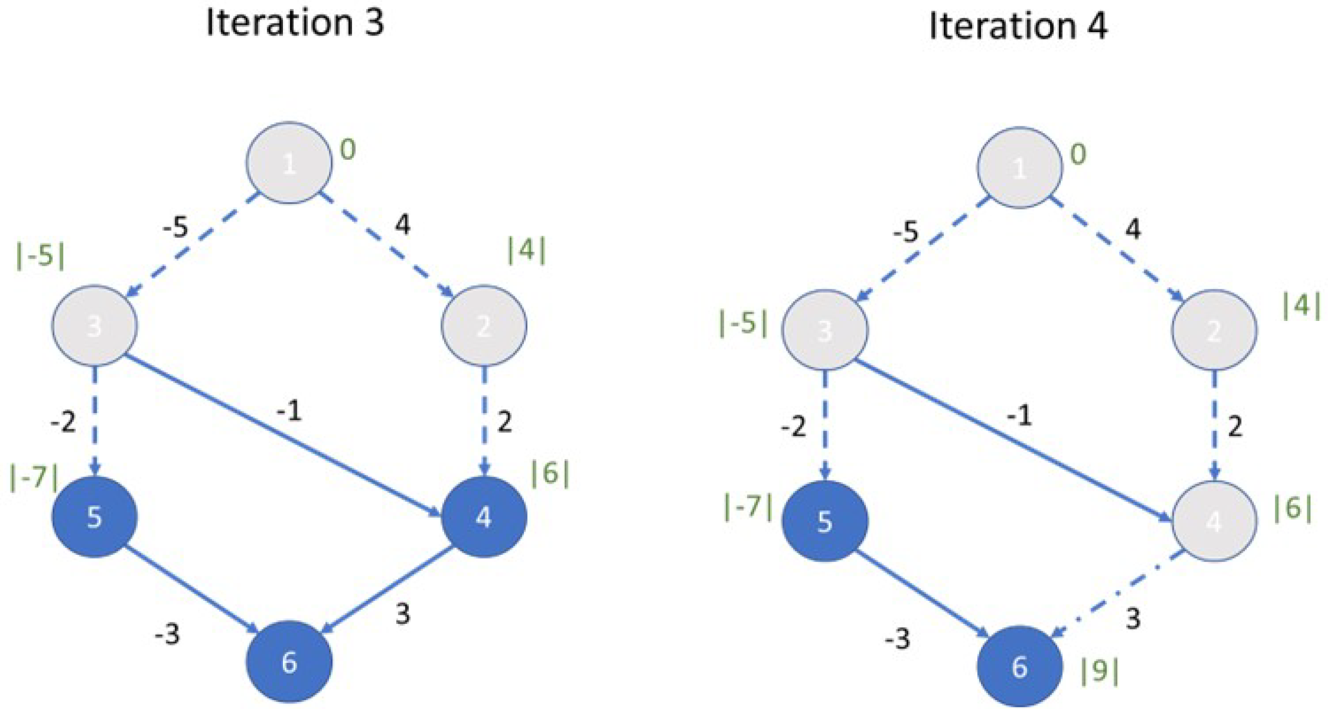
, to validate the computational results, an iterative heuristic algorithm is presented. Thus, in the present paper, two heuristic approaches are described, tested, and compared. The first is a two-step heuristic algorithm that implements a constructive heuristic algorithm in the first step ( C H a ) followed by an improvement phase ( I P a ). The constructive step is a modified version of the well-known Dijkstra algorithm to solve S P P [21], made necessary to deal with both positive and negative costs and the need to minimize the absolute value of the cost of the path. The second step of the algorithm I P a , starting from the feasible solution provided by C H a , tries to improve it using the information stored by I P a . In particular, starting from the destination node, algorithm I P a goes forward to evaluate new nodes that do not belong to the best-found path in C H a . A similar approach operating forward from the destination node is adopted in the definition of urban multimodal networks [22]. Note that the Dijkstra algorithm has often been combined in solution approaches for solving some variants of the S P P , as, for example, in [23,24,25]. The second heuristic algorithm is an iterative neighborhood search procedure [26] based on an initial randomly generated solution, improved thanks to I P a previously cited. Among the hundred generated starting solutions, the best one obtained is given for comparison with the previous method.
The computation efficiency of proposed algorithms is tested with randomly generated instances of different sizes, densities, and arc weights. Since no other tests obtained with previously proposed heuristics to solve C B P P are available as validation of the proposed algorithms, we have compared them.
The remaining of this paper is organized as follows. Section 2 presents the proposed algorithms for the C B P P , while Section 3 reports the computational experiments. Section 4 gives some conclusions and perspectives.

2. The Heuristic Algorithms

In the following, the two proposed heuristic algorithms are described.

2.1. The Two-Step Algorithm: Constructive and Improvement ( C H I P a )

As already said, the first proposed algorithm to solve the problem under investigation consists of two steps. The first step C H a is a constructive approach based on the Dijkstra algorithm [21]. This algorithm has in input a graph G ( N , A ) , an origin node o and a destination node d, and returns for each node of G the minimum cost for reaching it from node o. The second step I P a is an improvement algorithm that, starting from the feasible solution obtained by C H a , tries to improve it by using as input the solution provided by C H a related to the shortest path tree from the origin node to each node of the graph. Let us describe C H I P a in more detail.

2.1.1. C H a : Constructive Heuristic

C H a is designed to identify an acyclic path from an origin o node to a destination node d in which the sum of the arcs of the path is as close to zero as possible. This heuristic algorithm follows the scheme of the algorithm for determining the shortest path proposed by Dijkstra [21].
C H a is described in pseudocode in Algorithm 1. Looking at Algorithm 1, the reader can note that one of the differences with respect to Dijkstra’s algorithm is due to the extraction criteria of a node, as reported in line 9. In fact, we extract the lowest cost element in absolute value from Q, where Q denotes the set of nodes not yet analyzed. In particular, the extraction of destination node d from Q (see again line 9 of Algorithm 1), is performed only if d is the only node with a non-infinite cost. This allows the procedure to update the predecessor of node d as many times as possible in order to try to improve the current solution.
Algorithm 1 CHa ( G ( N , A ) , o, d).
1: Q
2: for each node n N  do
3:  c o s t [ n ]
4:  p r e v [ n ] N U L L
5:  Q Q { n }
6: end for
7: c o s t [ o ] 0
8: while Q do
9:  u node in Q with minimum | c o s t [ u ] |    ▹ (extract d from Q only if
   n Q / { d } : c o s t [ n ] < )
10:  Q Q { u }
11: for each neighbor n of u do
12:  if  n Q  then
13:    d c o s t [ u ] + c u n
14:   if  | d | < | c o s t [ n ] |  then
15:     c o s t [ n ] d
16:     p r e v [ n ] u
17:   end if
18:  end if
19: end if
20: end while
21: return c o s t , p r e v
In our algorithm, we examine the set Q of nodes as reported in line 12 of Algorithm 1, only if it is still present in Q to avoid processing the same node several times. This is implicitly done in Dijkstra’s algorithm because if a node has already been extracted from Q, it is not possible to reach it later with a lower cost.
Finally, as reported in line 14 of Algorithm 1, in the cost path evaluation from the origin node o, we compare the costs of reaching a node using the absolute value associated with the corresponding arc and select the minimum one.
Just to give an example of C H a , suppose to have to solve the C B P P from node 1 to node 6 of the graph reported in Figure 1. In the same figure are depicted two iterations of the algorithm. The first node selected from Q is node 2, with cost c 2 = 4 . The next selection is for node 3, with cost c 3 = | 5 | = 5 (that is less than the cost for reaching node 4, i.e., c 4 = c 2 + c 2 , 4 = | 6 | = 6 ). With two more iterations, reported in Figure 2, node 6 is selected from Q, and a feasible solution is found. The cost for reaching node 6 is 9, and the selected path is nodes 1-2-4-6. Looking at the graph, it is possible to find a better solution, that is, the path consisting of nodes 1-3-4-6 with a cost of 3. We try to improve the obtained solution (nodes 1-2-4-6) by using the improvement algorithm described in the next section.
Using a priority queue proposed in [27], the complexity of Dijkstra’s algorithm is equal to O ( | A | + | N | l o g | N | ) . Considering that the number of nodes extracted from Q does not change in our implementation, using a Fibonacci heap to represent Q, the computational complexity of C H a remains unchanged.
The last part of the constructive algorithm consists of the identification of a path and its cost evaluation. These procedures are described in Algorithms 2 and 3, respectively. In more detail, the Algorithm 2, here denoted as P a t h , is used to create a set P containing the nodes along the path that connects node o to node d within the tree previously created by C H a . The Algorithm 3 C o s t P a t h is used to compute the sum of the costs of the arcs along the path that connects node o to node d within this tree. Considering that, in the worst case, both Algorithms 2 and 3 must visit all the nodes of the graph G ( N , A ) , their computational complexity is O ( | N | ) .
Algorithm 2 Path (o, d, p r e v ).
1: n d
2: P { n }
3: repeat
4:  n p r e v [ n ]
5:  P P { n }
6: until n o
7: return P
Algorithm 3 CostPath (o, d, p r e v ).
1: n d
2: c o s t 0
3: repeat
4:  n p r e v [ n ]
5:  c o s t c o s t + c n n
6:  n n
7: until n o
8: return c o s t

2.1.2. I P a : Improvement Phase

The improvement Algorithm 4, here denoted I P a , is described below. The algorithm has been designed to improve the solution obtained by the constructive heuristic C H a , by exploiting the tree stored in p r e v . In particular, this algorithm inversely visits the path from o to d produced by C H a . Starting at node d (line 1), it enters a loop (line 3) that ends only when node o is reached. For each node n in the path, it tries to identify a new parent n (line 6) which allows it to improve the objective function (line 7). To avoid the creation of sub-cycles, it is tested that the new parent n is not a descendant of the current node n (line 8).
Algorithm 4 IPa ( G ( N , A ) , o, d, c o s t , p r e v ).
1: n d
2: c u r r C o s t c o s t [ d ]
3: while n o do
4:  n p p r e v [ n ]
5: for each arc ( n , n ) A  do
6:   d s c o s t [ n ] + c n n + C o s t P a t h ( n , d , p r e v )
7:  if  | d s | < | c u r r C o s t |  then
8:   if  P a t h ( n , d , p r e v ) P a t h ( o , n , p r e v ) =  then
9:     n p n
10:   end if
11:  end if
12: end for
13:  p r e v [ n ] n p
14:  n n p
15: end while
16: return p r e v , c u r r C o s t
Analyzing the computational complexity of this algorithm, we have a complexity of O ( | N | ) in line 3, having to iterate over a maximum of | N | nodes, and for the loop of line 5 forces the algorithm to visit a maximum of ( | N | 1 ) arcs, reaching a complexity of O ( | N | 2 ) . Finally, considering the complexity of the functions P a t h and C o s t P a t h we reach a computational complexity equal to O ( | N | 3 ) .
Just to give an idea of the I P a , in Figure 3 the starting solution and the first improvement iteration are reported.
In particular, starting from node 6, the algorithm searches for a node connected to 6, reached during the execution of C H a and not belonging to the current solution. The first (and unique) candidate is node 5. Before accepting node 5 and modifying the solution, the algorithm checks if passing through node 5 to reach node 6 from node 1 is cheaper than the current solution. This is not the case, thus node 5 is not selected. Moreover, going forward from node 6 to node 4, there is a candidate node 3. Connecting node 3 to 4 is convenient: the new path from the origin node 1 to node 3, plus the cost of the new arc connecting node 3 to node 4, and the cost from node 4 to the destination node 6 permits to improve the objective function that passes from |9| to |3|. This selection is accepted and the search continues going forward from node 3 to the origin. There are no more possibilities to improve the solution, thus the algorithm stops.

2.2. The Iterated Neighborhood Search Procedure

The second heuristic algorithm to solve the C B P P is an iterative neighborhood search procedure. A feasible solution is randomly generated and then it is improved. In the improvement phase, we use the improvement algorithm defined in Section 2.1.2. The obtained solution is stored and the process is iterated many times starting from a new random generated feasible solution. The iterated neighborhood search Algorithm 5, called R P , describes in detail the generation of the starting feasible solution. It identifies a random path between the origin node o and the destination node d, and creates a random spanning tree rooted in the origin node. The whole iterated process is described in Algorithm 6, called R P R . Note that i t = 100 different starting solutions are generated. At the end, the best improved solution is returned and used for the comparison with the previous method. Algorithm 7 describes the R a n d o m T r e e function used within the R P and R P R function code to generate a randomized rooted tree.
Algorithm 5 RP ( G ( N , A ) , o, d, i t ).
1: P
2: c o s t
3: for i t iterations do
4:  c o s t , p r e v R a n d o m T r e e ( G , o , d )
5: if  | C o s t P a t h ( o , d , p r e v ) | < | c o s t |  then
6:   c o s t C o s t P a t h ( o , d , p r e v )
7:   P P a t h ( o , d , p r e v )
8: end if
9: end for
10: return P
Algorithm 6 RPR ( G ( N , A ) , o, d, i t ).
1: P
2: c o s t
3: for i t iterations do
4:  c o s t , p r e v R a n d o m T r e e ( G , o , d )
5:  c u r r C o s t , p r e v I P ( G , o , d , c o s t , p r e v )
6: if  | C o s t P a t h ( o , d , p r e v ) | < | c o s t |  then
7:   c o s t C o s t P a t h ( o , d , p r e v )
8:   P P a t h ( o , d , p r e v )
9:  end if
10: end for
11: return P
Algorithm 7 RandomTree ( G ( N , A ) , o, d).
1: Q
2: for each node n N  do
3:  c o s t [ n ]
4:  p r e v [ n ] N U L L
5:  Q Q { n }
6: end for
7: c o s t [ o ] 0
8: while Q do
9:  u random node in Q
10:  Q Q { u }
11: for each neighbor n of u do
12:  if  c o s t [ n ] =  then
13:    d c o s t [ u ] + c u n
14:    c o s t [ n ] d
15:    p r e v [ n ] u
16:  end if
17: end for
18: end while
19: return c o s t , p r e v

3. Computational Experiments

In this section, we report the computational experimentation performed to validate the proposed algorithms. The computational tests were performed on a MacBook Pro (Apple Inc., Cupertino, CA, USA), with a 2.9 GHz Intel i9 (Intel Inc., Santa Clara, CA, USA) processor and 32 GB of RAM. In all tests, we used as input the two sets of instances reported in [12] and some new large random instances also generated, as described in [12].
The first set of instances, named G r i d , is characterized by complete square grids, where each node is connected to its four neighbors. The second set of instances, named R a n d , is characterized by randomly generated connected graphs with the average degree ranging from 2 to 20. All instances used in this section can be found at the link [28]. In the following, we will refer to these instances as G r i d [ R a n d ] n 1 n 2 , where n 1 represents the number of nodes and n 2 represents the percentage of arcs incident on each vertex. The third set of instances is an extension of the R a n d instances generated with the same criteria but with a number of nodes equal to 500 , 1000 , 2000 , and 5000.
The costs associated with the arcs of each instance were generated following 3 different schemes, based on a homogeneous distribution of randomly generated costs with different ranges, respectively, [ 10 , 10 ] , [ 100 , 100 ] and [ 1 K , 1 K ] .
Each row in the following tables reports the average of the results of five instances.
In the following different experimental campaigns are reported.

3.1. First Experimental Campaign: Small Instances

Small instances have been optimally solved by the mathematical model presented in [12], thus we are able to compare the results obtained by the proposed C H I P a algorithm with the optimal solutions. Thanks to the following results, it is possible to understand the behaviour of the proposed algorithm, in particular the effectiveness of I P a , and to compare G r i d and R a n d instances.
Table 1 shows the number of optimal solutions obtained, respectively, using C H a and C H I P a . Looking at Table 1, we can observe that I P a always improves the solutions obtained by C H a . This improvement is more evident for instances with costs [ 10 , 10 ] , while the number of optimal solutions remains almost the same for [ 1 K , 1 K ] instances. The two sets of instances ( G r i d and R a n d ) have the same behavior.
All instances can be solved in less than one millisecond.
Actually, in Table 2 are reported the absolute objective function values obtained at the end of C H a and C H I P a for instances with randomly generated costs in [ 10 , 10 ] , [ 100 , 100 ] and [ 1 K , 1 K ] . Note that, the optimal value for all instances is zero (as shown in [12]). From Table 2, it is evident that it is always possible to improve the objective function values using I P a after C H a . In particular, for the largest instances (i.e., last row of each group), both Grid and Rand, with costs in [ 10 , 10 ] , I P a is able to provide optimal solutions. On average, for grid instances, the improvements are 92.3%, 92.2% and 87.8%, respectively, for instances with costs [ 10 , 10 ] , [ 100 , 100 ] , and [ 1 K , 1 K ] . The improvements are about 70% for instances of type Rand_100, and about 82% for Rand_100. In all cases, the improvement is lower when costs are in [ 1 K , 1 K ] .
Finally, by comparing the results shown in Table 2 with the optimal values, that is for all these instances equal to zero, we can note that the optimality gap is larger for instances with costs in [ 1 K , 1 K ] .
In further computational experimentation, we solved instances whose optimal value of the objective function is not zero. In particular, the costs associated with the arcs of the corresponding graph are obtained as follows: a random cost is associated with each node in the range [0, 10,000]. Then, the cost of an arc is obtained by a 1 % random perturbation of the displacement of the costs. We will refer to this cost structure as P E L .
For this type of instance, we noted that the proposed algorithm did not provide good solutions, even if it performs very quickly. The best case corresponds to the Rand _100 _03 set of instances, for which the optimal value is 6005, while the solutions obtained at the end of C H a and C H I P a , respectively, are 6557 and 5431, thus corresponding to an optimality gap of 7%. Unfortunately, in the worst case, we have a set of instances (Rand_200_20) with the average optimal function value equal to 74, while our algorithm is not able to go down 2605. Note that, also in these cases, the computational time is negligible.
The above computational results suggest that the proposed algorithm can produce effective solutions in case of very large instances and when the cost of the arcs is generated uniformly. Instead, it appears that the algorithm cannot be used for instances with cost-structure P E L . It also seems that as the size of the instances increases, the quality of the solution produced improves, as does the number of optimal solutions identified.

3.2. Second Experimental Campaign: Large Instances

This experimental campaign is based on the third set of generated instances, a set of random, larger-sized instances, for which it is not possible to obtain the optimal solution by the mathematical model used to solve small instances.
These tests permit a better investigation of the behavior of the proposed C H I P a algorithm. The obtained results are compared with those of the iterated neighborhood search procedure. In these new sets of instances, the number of nodes ranges from 500 to 5000. For completeness, the following tables report also the results related to small instances. Note that tests have been executed with costs generated uniformly ([−10, 10], [−100, 100] and [1K, 1K]) and with cost structure P E L .
Table 3 shows the behavior of C H I P a as the size of the instances increases. The number of solutions with objective function values equal to zero is shown. Although we do not know the optimal solution for the generated large instances, obviously we can certify the optimality of the heuristic solution in case a solution with an objective function value equal to zero is identified. We can see that, as the size of the instance increases, the number of zero-solutions improves. The table shows that the proposed algorithm is able to identify 92% of optimal solutions for the solved instances (i.e., 167 on 180) in case of uniform cost distribution in [ 10 , 10 ] . In all instances with a number of nodes greater than or equal to 500, we can obtain the optimal solution. Moreover, with the increase in | N | also for the distribution of costs P E L we are able to identify numerous optimal solutions, with | N | = 5000 we identify at least 25 optimal solutions (i.e., 83%).
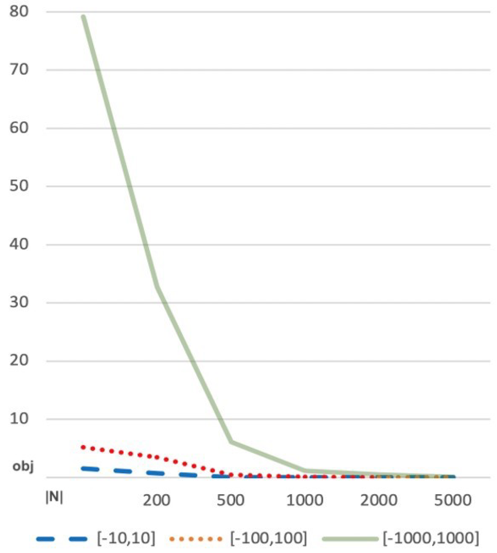
Table 4 shows the average value of the objective function for the same scenario as Table 3. The data contained in this table are used in Figure 4 to highlight how the solution produced improves as the size increases.
Table 5 reports the CPU time in milliseconds. The computational time required to produce a solution using the C H I P a is less than half a second even for instances with 5000 nodes. These computational times suggest that the average number of iterations of the algorithm is significantly less than the number of iterations associated with the computational complexity of the worst case O ( | N | 3 ) . Table 6 shows the average number of iterations performed by I P a . The I O M column is useful to understand how many iterations, on average, are performed for every million theoretical iterations associated with the worst case O ( | N | 3 ) . Figure 5 shows the relationship between the number of iterations and the number of nodes in the graph. For the set of instances used, the trend as | N | increases appears linear.
In the following tables, the results obtained by C H I P a are compared with those obtained by using the iterated neighborhood search procedure described in Section 2.2. In each Table, both the best among the first random paths ( R P ) and the best path after the improvement phase ( R P R ) are reported.
Table 7 and Table 8 show, respectively, the number of optimal solutions and the computational times in milliseconds, identified by C H I P a , R P and R P R .
It can be seen from these tables that C H I P a produces the maximum number of optimal solutions in about 1 50 of the computational time required by the R P and R P R iterative techniques.
In particular, C H I P a is able to find more 30% optimal solutions than R P R for costs [−100, 100] and P E L , and about 180% for cost [−1K, 1K].
These results also show that I P a applied to the R P significantly increases the number of optimal solutions identified by the R P , passing from 181 to 319 optimal solutions identified; the greatest effect is on instances with cost P E L and [−1K, 1K].

4. Conclusions and Outline Future Works

In this paper, we addressed the Cost-Balanced Path Problem, which fits into the class of the balanced combinatorial optimization problems. A two-step heuristic algorithm is proposed for solving this variant of the classical Shortest Path Problem. An iterative heuristic has been developed to compare the produced solutions. To the authors’ knowledge, this is the first research work related to heuristic algorithms to solve the C B P P . This two-step heuristic algorithm ( C H I P a ) is able to find feasible solutions in a negligible computational time and is particularly suitable for large-sized graphs. In fact, it is worth noting that by executing the constructive and the improvement heuristic algorithms consecutively, we can always find a larger number of optimal solutions in a very short CPU time. In particular, comparing the C H I P a solutions with those obtained by the iterative algorithm, which is a simple and fast heuristic method. Since the C B P P can be applied in many real-life problems for which only large size instances are required, such as vehicle battery level, altitude change, and cargo problems among others, as future work the authors will work on the development of a metaheuristic to be able to improve the goodness of the solutions for many types of instances of the C B P P .

Author Contributions

D.A., C.C. and A.S. contributed equally to this work. All authors have read and agreed to the published version of the manuscript.

Funding

This research received no external funding.

Institutional Review Board Statement

Not applicable.

Informed Consent Statement

Not applicable.

Data Availability Statement

Data available on request.

Conflicts of Interest

The authors declare no conflict of interest.

Abbreviations

The following abbreviations are used in this manuscript:
SPPShortest Path Problem
CBPPCost-Balanced Path Problem
TSPTravelling Salesman Problem
MILPMixed Integer Linear Programming
CHaConstructive Heuristic algorithm
IPaImprovement Phase algorithm

References

  1. Martello, S.; Pulleyblank, W.R.; Toth, P.; de Werra, D. Balanced optimization problems. Oper. Res. Lett. 1984, 3, 275–278. [Google Scholar] [CrossRef]
  2. Duin, C.W.; Volgenant, A. Minimum deviation and balanced optimization: A unified approach. Oper. Res. Lett. 1991, 10, 43–48. [Google Scholar] [CrossRef]
  3. McGovern, S.M.; Gupta, S.M. A balancing method and genetic algorithm for disassembly line balancing. Eur. J. Oper. Res. 2007, 179, 692–708. [Google Scholar] [CrossRef]
  4. Levitin, G.; Rubinovitz, J.; Shnits, B. A genetic algorithm for robotic assembly line balancing. Eur. J. Oper. Res. 2006, 168, 811–825. [Google Scholar] [CrossRef]
  5. Papadopoulos, H.T.; Vidalis, M.I. Minimizing WIP inventory in reliable production lines. Int. J. Prod. Econ. 2001, 70, 185–197. [Google Scholar] [CrossRef]
  6. Arbib, C.; Lucertini, M.; Nicolò, F. Workload balance and part-transfer minimization in flexible manufacturing systems. Int. J. Flex. Manuf. Syst. 1991, 3, 5–25. [Google Scholar] [CrossRef]
  7. Bhagwat, R.; Sharma, M.K. Performance measurement of supply chain management using the analytical hierarchy process. Prod. Plan. Control. 2007, 18, 666–680. [Google Scholar] [CrossRef]
  8. Babaioff, M.; Walsh, W.E. Incentive-compatible, budget-balanced, yet highly efficient auctions for supply chain formation. Decis. Support Syst. 2005, 39, 123–149. [Google Scholar] [CrossRef]
  9. Kaspi, M.; Kesselman, U.; Tanchoco, J.M.A. Optimal solution for the flow path design problem of a balanced unidirectional AGV system. Int. J. Prod. Res. 2002, 40, 389–401. [Google Scholar] [CrossRef]
  10. Chen, H.; Ye, H.Q. Asymptotic optimality of balanced routing. Oper. Res. 2012, 60, 163–179. [Google Scholar] [CrossRef] [Green Version]
  11. Li, X.; Wei, K.; Aneja, Y.P.; Tian, P.; Cui, Y. Matheuristics for the single-path design-balanced service network design problem. Comput. Oper. Res. 2017, 77, 141–153. [Google Scholar] [CrossRef]
  12. Ambrosino, D.; Cerrone, C. The Cost-Balanced Path Problem: A Mathematical Formulation and Complexity Analysis. Mathematics 2022, 10, 804. [Google Scholar] [CrossRef]
  13. Turner, L. Variants of the shortest path problem. Alg. Oper. Res. 2011, 6, 91–104. [Google Scholar]
  14. Greco, S.; Pavone, M.F.; Talbi, E.-G.; Vigo, D. Metaheuristics for combinatorila optimization. In Advances in Intelligent Systems and Computing; Springer: Cham, Switzerland, 2021. [Google Scholar]
  15. Akbay, M.; Kalayci, C. A variable neighborhood search algorithm for cost-balanced travelling salesman problem. In Metaheuristics for Combinatorila Optimization Advances—Intelligent Systems and Computing; Springer: Cham, Switzerland, 2021; pp. 23–36. [Google Scholar]
  16. Larusic, J.; Punnen, A.P. The balanced traveling salesman problem. Comput. Oper. Res. 2011, 38, 868–875. [Google Scholar] [CrossRef]
  17. Pierotti, J.; Ferretti, L.; Pozzi, L.; van Essen, J.T. Adaptive Iterated Local Search with Random Restarts for the Balanced Travelling Salesman Problem. In Metaheuristics for Combinatorila Optimization Advances—Intelligent Systems and Computing; Springer: Cham, Switzerland, 2021; pp. 36–56. [Google Scholar]
  18. Dong, X.; Xu, M.; Lin, Q.; Han, S.; Li, Q.; Guo, Q. IT algorithm with local search for large scale multiple balanced traveling salesmen problem. Knowl.-Based Syst. 2021, 229, 107330. [Google Scholar] [CrossRef]
  19. Moharam, R.; Morsy, E. Genetic algorithms to balanced tree structures in graphs. Swarm Evol. Comput. 2017, 32, 132–139. [Google Scholar] [CrossRef]
  20. Zhou, J.; Kang, L.; Shan, E. Two paths location of a tree with positive or negative weights. Theor. Comput. Sci. 2015, 607, 296–305. [Google Scholar] [CrossRef]
  21. Dijkstra, E.W. A note on two problems in connexion with graphs. Numer. Math. 1959, 1, 269–271. [Google Scholar] [CrossRef]
  22. Ambrosino, D.; Sciomachen, A. An Algorithmic Framework for Computing Shortest Routes in Urban Multimodal Networks with Different Criteria. Procedia Soc. Behav. Sci. 2014, 108, 139–152. [Google Scholar]
  23. Dinitz, Y.; Itzhak, R. Hybrid Bellman–Ford–Dijkstra algorithm. J. Discret. Alg. 2017, 42, 35–44. [Google Scholar] [CrossRef]
  24. Lewis, R. Algorithms for Finding Shortest Paths in Networks with Vertex Transfer Penalties. Algorithms 2020, 13, 269. [Google Scholar] [CrossRef]
  25. Abdelghany, H.M.; Zaki, F.W.; Ashour, M.M. Modified Dijkstra Shortest Path Algorithm for SD Networks. Int. J. Electr. Comput. Eng. Syst. 2022, 13, 203. [Google Scholar] [CrossRef]
  26. Carrabs, F.; Cerrone, C.; Cerulli, R.; Silvestri, S. The rainbow spanning forest problem. Soft Comput. 2018, 22, 2765–2776. [Google Scholar] [CrossRef]
  27. Fredman, M.L.; Tarjan, R.E. Fibonacci heaps and their uses in improved network optimization algorithms. J. ACM 1987, 34, 596–615. [Google Scholar] [CrossRef]
  28. Test Instances. Available online: https://github.com/CarmineCerrone/CostBalancedPathProblem (accessed on 12 September 2022).
Figure 1. A simple example of two iterations of C H a .
Algorithms 15 00364 g001
Figure 2. The last iterations of C H a .
Algorithms 15 00364 g002
Figure 3. An example of I P a .
Algorithms 15 00364 g003
Figure 4. Objective function values obtained by C H I P a compared to the size of the instances.
Algorithms 15 00364 g004
Figure 5. Relationship between the number of I P a iterations and | N | .
Algorithms 15 00364 g005
Table 1. Number of optimal solutions identified—instances with random costs.
Instance CHa CH IPa
[−10, 10][−100, 100][−1K, 1K][−10, 10][−100, 100][−1K, 1K]
Grid_100_10200210
Grid_225_15000310
Grid_400_20100500
# OPT3001020
Rand_100_02000100
Rand_100_03011311
Rand_100_04110410
Rand_100_05200310
Rand_100_10310530
Rand_100_20500520
# OPT11312181
Rand_200_02200310
Rand_200_03200410
Rand_200_04000500
Rand_200_05200400
Rand_200_10420530
Rand_200_20510521
# OPT15302671
Table 2. Absolute objective function values obtained—instances with random costs.
Instance CHa CH IPa
[−10, 10][−100, 100][−1K, 1K][−10, 10][−100, 100][−1K, 1K]
Grid_100_103.620.8393.80.63.458.0
Grid_225_154.257.2506.00.44.453.2
Grid_400_204.057.0448.60.02.853.2
AVG3.945.0449.50.33.554.8
Rand_100_025.054.0782.21.415.2249.0
Rand_100_034.040.8253.62.05.662.6
Rand_100_043.421.2225.20.24.449.0
Rand_100_050.812.0239.60.64.064.4
Rand_100_100.44.240.40.00.837.4
Rand_100_200.05.241.20.01.212.8
AVG2.322.9263.70.75.279.2
Rand_200_022.030.2314.40.66.641.6
Rand_200_030.818.2237.00.29.4123.2
Rand_200_042.217.0128.20.02.210.4
Rand_200_051.415.073.20.21.04.6
Rand_200_100.23.031.00.01.212.6
Rand_200_200.00.824.80.00.63.8
AVG1.114.0134.80.23.532.7
Table 3. Number of optimal solutions identified by C H a and C H I P a —large instances.
|N| CHa CH IPa
[−10, 10][−100, 100][−1K, 1K]PEL[−10, 10][−100, 100][−1K, 1K]PEL
1001131021810
2001530026711
50024500301833
10002514203028136
200030172030302013
500030255030302725
#OPT137671001671216548
Table 4. Absolute objective function values— C H a and C H I P a —large instances.
|N| CHa CH IPa
[−10, 10][−100, 100][−1K, 1K]PEL[−10, 10][−100, 100][−1K, 1K]PEL
1002.322.9263.73165.40.75.279.23057.5
2001.114.0134.83800.40.23.532.73583.8
5000.65.845.63086.20.00.46.12462.2
10000.22.118.13782.40.00.11.12776.3
20000.00.814.03129.20.00.00.51374.0
50000.00.33.23461.10.00.00.1272.3
AVG0.77.779.93404.10.11.520.02254.4
Table 5. CPU time (milliseconds) of the proposed C H I P a .
Instance CH IPa
[−10, 10][−100, 100][−1K, 1K]PEL
Rand_100_020000
Rand_100_030000
Rand_100_040000
Rand_100_050000
Rand_100_100000
Rand_100_200000
Rand_200_020000
Rand_200_030000
Rand_200_040010
Rand_200_050000
Rand_200_100011
Rand_200_200001
Rand_500_021010
Rand_500_031001
Rand_500_040111
Rand_500_050111
Rand_500_101211
Rand_500_203333
Rand_1000_022222
Rand_1000_032332
Rand_1000_042333
Rand_1000_054444
Rand_1000_107878
Rand_1000_2011111112
Rand_2000_028999
Rand_2000_0310121211
Rand_2000_0412151414
Rand_2000_0513151514
Rand_2000_1025272725
Rand_2000_2048515355
Rand_5000_0242505253
Rand_5000_0357677165
Rand_5000_0473859083
Rand_5000_0588103112101
Rand_5000_10217204202201
Rand_5000_20366350371328
AVG27.628.529.627.7
Table 6. Average and theoretical I P a (worst case) iterations, and CPU time.
|N|IterationsIOMTime (ms)
1001281280
200392490
5001966161
1000464057
200011,303127
500026,3050143
Table 7. Comparison of the number of optimal solutions identified.
|N|[−10, 10][−100, 100][−1K, 1K]PEL
C H I P a 10021810
20026711
500301833
10003028136
200030302013
500030302725
#OPT1671216548
RP10025810
20023520
50022500
100021700
200022700
500026520
#OPT1393750
RPR100251110
200271131
500271253
1000291625
20002822310
50003021918
#OPT166932337
Table 8. Comparison of the CPU time (milliseconds).
|N|[−10, 10][−100, 100][−1K, 1K]PEL
C H I P a 1000000
2000000
5001111
10005555
200019222221
5000140143150138
AVG28283028
RP1001111
2002333
50013242625
1000113164195206
2000776118312941288
50002263719273597359
AVG528142814801480
RPR1001111
2003333
50025262625
1000210192195208
20001315122413001289
50008025736973737361
AVG1596146914831480
Publisher’s Note: MDPI stays neutral with regard to jurisdictional claims in published maps and institutional affiliations.

