Enhanced Maximum Power Point Techniques for Solar Photovoltaic System under Uniform Insolation and Partial Shading Conditions: A Review

Abstract

In the recent past, the solar photovoltaic (PV) system has emerged as the most promising source of alternative energy. This solar PV system suffers from an unavoidable phenomenon due to the fluctuating environmental conditions. It has nonlinearity in I-V curves, which reduces the output efficiency. Hence, the optimum maximum power point (MPP) extraction of the PV system is difficult to achieve. Therefore, for maximizing the power output of PV systems, a maximum power point tracking (MPPT) mechanism, which is a control algorithm that can constantly track the MPP during operation, is required. However, choosing a suitable MPPT technique might be confusing because each method has its own set of advantages and disadvantages. Hence, a proper review of these methods is essential. In this paper, a state-of-the-art review on various MPPT techniques based on their classifications, such as offline, online, and hybrid techniques under uniform and nonuniform irradiances, is presented. In comparison to offline and online MPPT methods, intelligent MPPT techniques have better tracking accuracy and tracking efficiency with less steady state oscillations. Unlike online and offline techniques, intelligent methods track the global MPP under partial shade conditions. This review paper will be a useful resource for researchers, as well as practicing engineers, to pave the way for additional research and development in the MPPT field.

1. Introduction

1.1. Motivation and Incitement

Solar energy has become the most popular renewable energy source, since it can be used in any location and is available every day. Because of its simple structure, low pollution, low or no carbon greenhouse emissions, and low maintenance costs, it has become a dominant renewable source [1]. Solar power is currently the world’s preferred alternative energy source [2]. Nonetheless, the solar PV system suffers from the unavoidable problem of current and voltage nonlinearity, which occurs primarily in partially shaded conditions (PSC). In general, PV systems have a unique operating point where the power is at its maximum. Hence, the PV system needs to operate at this point to harvest the maximum efficiency [3]. For maximizing output power under all abnormal conditions, the PV system takes account of the MPPT mechanism.

1.2. Research Gap

In the recent decade, many research proposals on MPPT for PV systems have been introduced. A few MPPT approaches have been proposed that are based on uniform irradiances, while others have been proposed that are based on partial shading conditions. However, choosing MPPT for specific PV system designs and situations might be confusing, since each approach has its own set of benefits and drawbacks. Numerous reviews on the subject have been published to aid academics and field engineers to choose the optimal MPPT for a certain PV system. The conventional MPPT techniques are regarded by the majority of studies as a successful way of obtaining maximum output power from solar PV systems under nonuniform irradiation [4,5,6,7,8,9]. Partial shadowing or mismatched sun irradiation conditions were also explored in a few works of literature [10,11,12,13]. Furthermore, Salam et al. [14] proposed swarm intelligence-based MPPT approaches as a feasible alternative. Although, only a few papers [9,15] have focused on MPPT under uniform solar irradiation and PSC.

In the literature, the various types of conventional MPPT techniques developed so far are fractional short circuit current (FSCC) [16,17], fractional open circuit voltage (FOCV) [18], curve fitting (CF) [19], constant voltage (CV) [20], hill climbing (HC) [21], incremental conductance (INC) [22] and ripple correlation control (RCC) [23] methods. The main shortcoming of the FSCC and FOCV methods is that they are less accurate; hence, they are primarily used in low-power applications [24]. While well-known approaches such as P&O, HC, and INC can only measure maximum power for uniform irradiation, these techniques completely fail when partial shade occurs, that is, when panels in an array receive uneven irradiation [25,26,27]. Additionally, these approaches exhibit poor convergence, slow tracking speed, and excessive steady-state oscillations. As a result, traditional methods must be combined with alternative methods to track MPP under partial shading conditions (PSC). In the meantime, a novel adaptive P&O technique that uses variable step sizes rather than fixed step sizes is being developed [17,28]. Despite the fact that the preceding modifications have improved their performance, they are insufficient under all operating conditions [29,30,31].

To address the shortcomings of conventional MPPT techniques, swarm intelligence techniques have been introduced in the field of solar PV systems research [32,33,34]. These approaches are regarded as the best options for non-linear optimization because of multiple advantages, such as (a) wide exploration in search space; (b) ability to manage nonlinearity and (c) the coherence of their ability to locate global optimal regions. The MPPT approaches that fall under swarm intelligence techniques are artificial neural network (ANN) [35,36,37], fuzzy logic control (FLC) [38,39,40,41], bee colony search algorithm [42,43], differential evaluation [44,45], particle swarm optimization (PSO) [46,47,48,49,50,51,52], cuckoo search [53,54], genetic algorithm (GA) [55,56,57,58,59], fireflies algorithms [60], ant colony optimization [61,62], chaotic approach [63], nonlinear control [64], and random Search methods [65]. Furthermore, under partially shadowed conditions, these algorithms are substantially affected in terms of reaching the global maximum [66]. Because the quantity of required training is fairly extensive, its execution is made even more difficult. Similarly, Fibonacci [66] and DIRECT MPPT [67]-based techniques have similar drawbacks, making them unsuitable for achieving global optimal values. ANN and FLC are two soft computing technologies that are knowledge-based systems that require specific knowledge to implement the algorithm. ANN and FLC are effective at tracking MPP, but they require a lot of memory to train and implement rules. The FLC method, in particular, has the significant drawback of being unable to modify the rules once they have been defined.

Recently, many researchers have proposed hybrid MPPT methods and new optimization algorithms based on MPPT techniques. The ABC-P&O-based hybrid MPPT method decreases maximum overshoot by 30% when compared to the standard ABC-based MPPT method. However, the proposed method was tested with only two PV modules for PSCs [68]. A hybrid MPPT technique that included a particle swarm optimization approach and a cooperative ANN to maximize the PV system’s output power was developed. The ANN predicts the quantity of solar insolation and cell temperature, whereas the PSO optimizes power generation and tracks the MPP of the PV system under changing climatic circumstances [69]. The authors in ref. [70] have proposed various MPPT methods based on the Bat algorithm, such as Bat assisted P&O, Bat assisted Beta, and Bat assisted INC. However, it has very slow convergence, i.e., slow tracking speed, and also produces more oscillations at a steady state. To address this, an improved grey wolf optimizer (GWO) to extract global MPP under partial shade was developed, which gives a faster convergence speed. However, initial oscillations and a long settling time are present [71]. In ref. [72], the authors presented an enhanced Moth flame optimization (MFO) technique for obtaining maximum power under dynamic operating situations. This method improves tracking efficiency convergence speed. It is, however, more complicated, and it results in substantial initial steady-state oscillations.

1.3. Contribution

As mentioned above, there are conventional and swarm intelligence-based MPPT techniques in which a few deal with uniform irradiance conditions, and others deal with partial shading conditions in the literature. However, choosing a suitable MPPT method might be confusing because each technique has its own set of advantages and disadvantages. Consequently, a thorough review of these methods is necessary.

Recognizing the crucial importance of MPPT, various researchers made an effort to combine their findings and present them as reviews in [73,74,75,76,77], taking into account the function of MPPT in solar PV systems. The approaches discussed in the literature cannot be conclusive because these reviews are out-of-date and date back to before 2017. Additionally, in recent years, we have witnessed a notable rise in novel approaches for both traditional and optimization techniques. A critical assessment and analysis are, therefore, essential to complete the MPPT study with current methodologies and to cover the undiscovered ways.

For this purpose, it requires writing a review paper on recent MPPT methods based on uniform and nonuniform irradiance conditions. This review paper provides MPPT techniques classifications based on the tracking MPP under normal and abnormal conditions, such as offline, online, and intelligent MPPT techniques. It furnishes the complete details and comparison of these techniques. This paper also provides a comprehensive evaluation of each technique based on the following factors: (1) tracking accuracy, (2) efficiency, (3) complexity, (4) parameter tuning, and (5) PV array dependency. Furthermore, this review paper will be a useful resource for researchers, as well as practicing engineers, to pave the way for future research and development in the field of MPPT. The rest of the paper is organized as follows.

After this introduction part, the solar PV modeling and its characteristics are presented in Section 2. Section 3 presents MPPT techniques classifications and Section 4 deals with the comparative study of various MPPT techniques and their merits and demerits of MPPT techniques. Finally, Section 5 presents the conclusion of this research study.

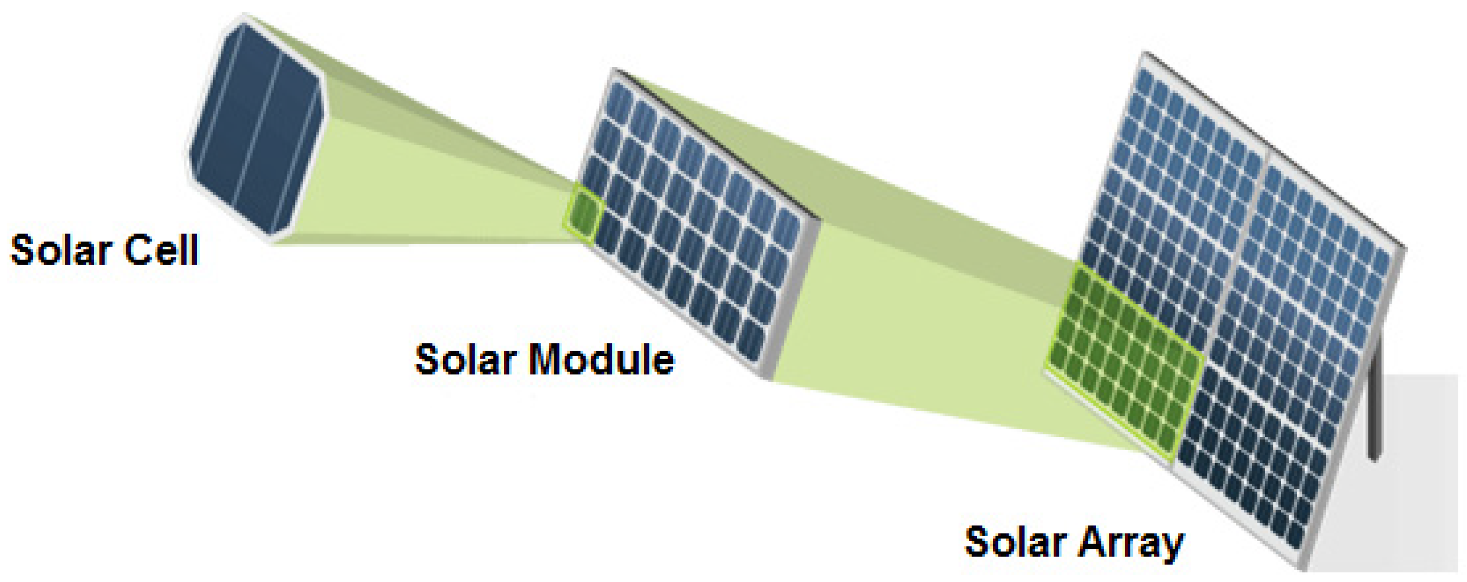
2. Solar PV Modeling and Characteristics

2.1. PV Cell Model

PV cell is a fundamental unit that uses the photovoltaic effect to turn solar energy into electrical energy. When exposed to sunlight, the PV cell generates electrical energy. The equivalent circuit of a typical PV cell contains series and shunt resistances, as presented in Figure 1. The single diode model is the most accurate of the many PV cell modeling methods. The KCL can be used to obtain the PV cell output current, I_PVC [78] as follows:

$$I_{PVC}=I_{LC}-I_d-\frac{V_{PVC}+R_S\ast I_{PVC}}{R_{SH}}$$

(1)

I_LC stands for light generated current (A), I_d for diode current (A), V_PVC for photovoltaic cell voltage (V) and R_S and R_SH are the series and shunt resistances of the PV cell (Ω).

When a PV cell is exposed to insolation and ambient temperature, the light-current, I_LC, is expressed as follows:

$$I_{LC}=\frac{G}{G_{ref}}\left[I_{LCref}+{\mu }_{sc}\left(T_{cell}-T_{ref}\right)\right]$$

(2)

T_cell and T_ref are the cell and standard temperatures in Kelvin (K), G for irradiance (w/m²), and µ_sc for the temperature coefficient.

Additionally, the diode current I_d is

$$I_d=I_o\left(e^{\frac{V_{PVC}+R_S\ast I_{PVC}}{V_t}}-1\right)$$

(3)

where V_t denotes thermal voltage (V).

The Io diode saturation dark current is proportional to temperature can be expressed as

$$I_o=I_{o,ref}{\left(\frac{T_{cell}}{T_{ref}}\right)}^3\exp \left[\left(\frac{q{\epsilon }_G}{A.K}\right)\left(\frac{1}{T_{ref}}-\frac{1}{T_{cell}}\right)\right]$$

(4)

A standard PV cell only produces 0.6 V, which is extremely low, so many cells are usually connected in series and parallel to form a PV module (panel) to raise the voltage to a level appropriate for the application, as shown in Figure 2. A typical rooftop solar panel has 60 cells, resulting in a 36 V open circuit voltage. To increase the system voltage, multiple panels (or modules) are connected in series for larger systems [79]. Parallel connections of modules can be present in an array of multiple solar panels, but parallel connections make sense only if the voltage is small. A series connection raises the voltage while holding the current constant, while a parallel connection raises, the current while keeping the voltage constant. Series connection is more effective than parallel connection because losses increase as the current increases.

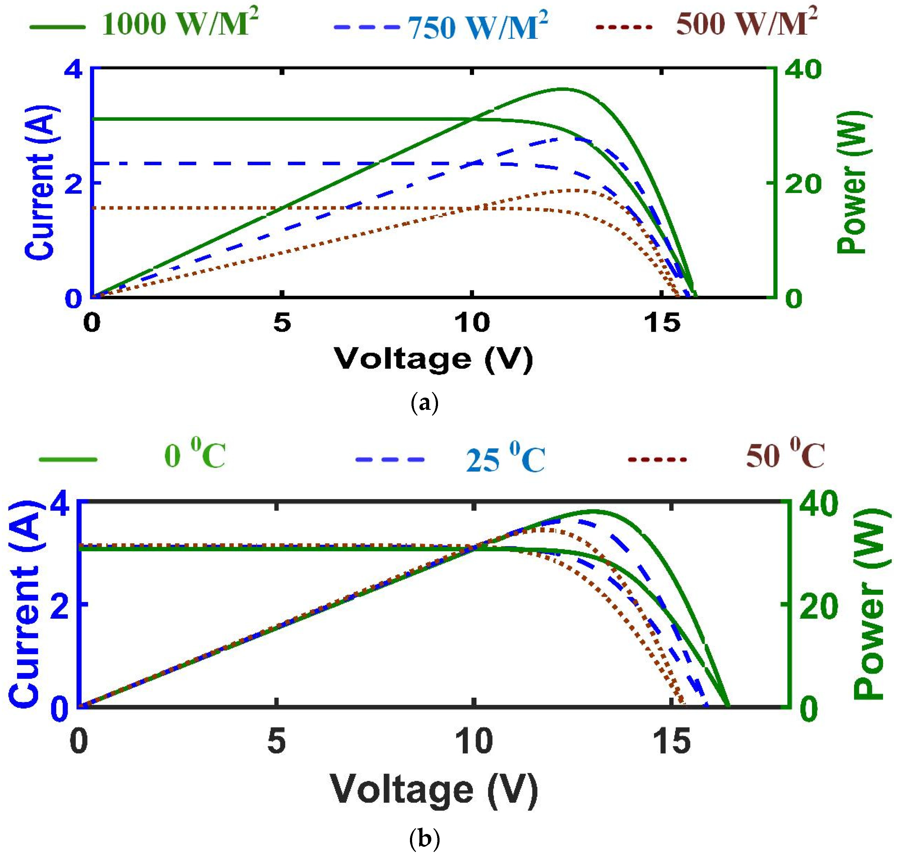
2.2. Characteristics of a PV System

Generally, the PV panel characteristics are described by I-V and P-V curves, as presented in Figure 3. It is worth noting that there is a specific operating point at which the output power is at its maximum. This unique point is referred to as the maximum power point (MPP) and is denoted by the letters MPP in the I-V and P-V curves. Due to the PV panel’s low efficiency, PV systems must always operate close to the MPP in order to gather the greatest amount of energy [80,81].

However, the performance of the PV panel can easily be affected by climatic conditions. The short circuit current is linearly dependent on the solar irradiance level, whereas the open-circuit voltage is strongly influenced by the cell temperature [82,83]. Figure 4a depicts the PV characteristics for changing irradiance and Figure 4b depicts the PV characteristics for changing temperature.

2.3. Solar PV System under Partial Shading

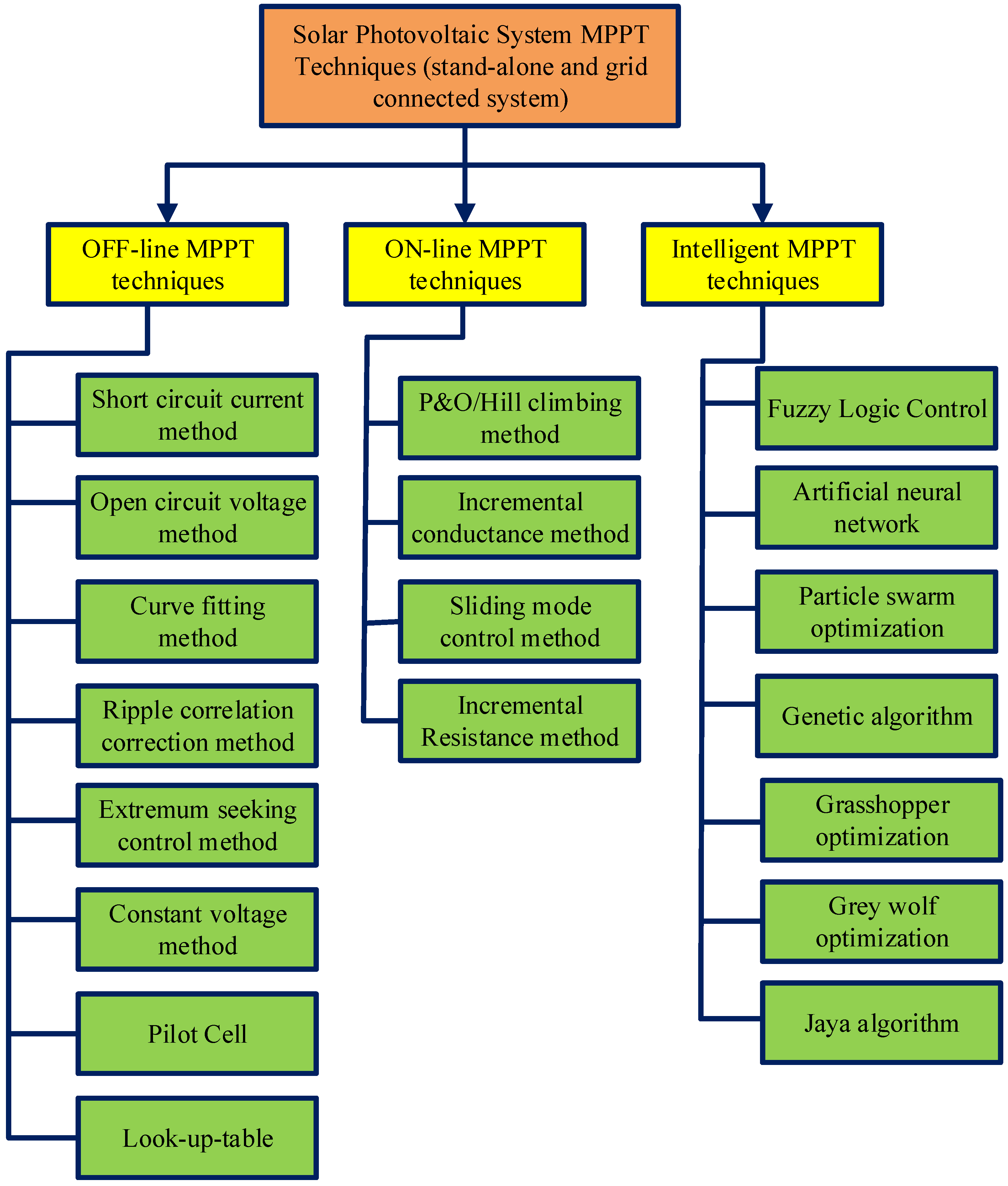
The performance of the PV array is also affected by the change in irradiance from panel to panel due to shadows of passing clouds, trees, nearby buildings, changes in climate, disposition of dust, the aging effect of the panel, etc [84,85]. Therefore, partial shading conditions (PSC) can occur in the PV system due to any of the above reasons. When the PSC takes place in the PV system, the voltage–power (V-P) curve produces the only peak or multiple peaks [86,87,88,89,90]. This single peak and multiple peaks on V-P curves depend on sunlight irradiances on the panels of the PV system. If all the PV panels receive the same irradiance, then there is only a peak on the P-V curve. If the PV panels (one or two or all) face the shadow effect, then there are multiple peaks on the P-V curve of the PV system. Figure 5 shows the P-V curves of the PV system under various shading conditions. As a result, the operating point that meets the MPP criterion also changes depending on the ambient conditions. For maximizing the power output of PV systems, an MPPT mechanism, which is a control algorithm that can constantly track the MPP during operation, is required [91].

3. MPPT Techniques

The MPPT technique is an electronic system that provides the duty cycle to the power conversion device in order to achieve peak power generation. As observed in Figure 6, MPPT is also well-known as an MPP matching device that is positioned between the PV array and the power converter [92,93,94]. Different inverter systems, external grids, battery banks, and other electrical loads interact differently with solar PV systems. The main issue that MPPT attempts to solve is the fact that the efficiency of power transmission from the solar cell is dependent on the quantity of sunlight, the amount of shade, the temperature of the solar panel, and the electrical characteristics of the load. The load characteristic impedance provides the maximum power transmission changes when these variables change. To maintain the best efficiency of power transfer as the load characteristic changes, the system is optimized. The maximum power point refers to this ideal load property (MPP). MPPT is the process of adjusting the load characteristic as the conditions change. Circuits can be designed to present optimal loads to the photovoltaic cells and then convert the voltage, current, or frequency to suit other devices or systems. The MPP tracking starts with an initial duty cycle. The input current I_PV and voltage V_PV of the boost converter are measured to calculate the SPVS power P_PV (k). Now, based on initial changes in power, the controller increases the duty cycle. At this stage, new I_PV and V_PV are measured to calculate new power P_PV (k + 1). Based on present and past information on SPVS power, the controller decides to decrease or increase the duty cycle. This process of tracking is continuous until the MPP is reached.

However, there are other important considerations when constructing MPPT techniques for PV systems, including efficiency, kind of implementation, complexity, lost energy, and cost [95]. Based on these, various MPPT approaches have been created and classified into three main groups, namely (i) offline or indirect MPPT techniques; (ii) online or direct MPPT techniques; (iii) intelligent MPPT techniques. A broad classification of MPPT techniques is shown in Figure 7.

3.1. Off-Line MPPT Techniques

The off-line MPPT method measures the short circuit current or the open circuit voltage by disconnecting the PV panel from the system (also referred to as off-line parameters). Since the PV panel is disconnected from the rest of the system during the calculation, it is referred to as off-line MPPT. These MPPT techniques do not continuously track the current or voltage; instead, they measure MPP based on apriori data. These methods have the major benefit of requiring fewer voltage and/or current sensors. The MPPs for changing insolation and temperatures are not precisely tracked by such systems. The following methods belong to this category: curve fitting (CF) [19], look-up-table (LUT) [96], pilot cell (PC) [97], fractional short-circuit current (FSCC) [98], and fractional open-circuit voltage (FOCV) [99].

The CF method uses a mathematical function to approximate the power characteristic of photovoltaic modules. To build a mathematical model and equation to explain the output characteristics, all manufacturing information and data are needed [19]. Equation (5) is used to measure the PV module characteristic, where a, b, c, and d are the coefficients determined by sampling the I_PV, V_PV, and P_PV [100]. After calculating these coefficients, the voltage at which the power achieves maximum is determined using Equation (6).

$$P_{PV}=a{V}_{PV}^3+b{V}_{PV}^2+c{V}_{PV}+d$$

(5)

$$V_{MP}=\frac{-b\pm \sqrt{b^2-3ac}}{3a}$$

(6)

However, due to the high complexity of the measurement, this approach is somewhat difficult. Every parameter of the formula must be calculated based on atmospheric conditions, manufacturing technology, and the material used to construct the cell. Estimating optimum operating conditions takes a lot of time and effort.

In the look-up table method, the PV module current (I_PV) and voltage (V_PV) are measured to track the MPP. Technical information about the PV panel, such as the output voltage for varying irradiance and temperature levels, is stored for various climatic situations. The lookup method then tracks the MPP by comparing the measured V_PV and I_PV with the stored data. As a result, a significant amount of data is stored in the lookup memory for reliable MPP monitoring and increased productivity [96]. This approach is complicated and error-prone because it requires a large amount of data collection, storage, and several sensors to monitor the precise MPP.

In a pilot cell algorithm, a constant voltage or constant current approach is used, where the V_OC is measured using a PC rather than the PV module/array [97]. As shown in Equation (7), the V_OC of the pilot cell is determined by multiplying a constant (K₁). The constant K₁ is pre-determined to track the array’s MPP in response to variations in temperature or irradiances.

$$V_{ref}=K_1\times V_{oc}\left(pilot cell\right)$$

(7)

where K₁ < 1.

In addition, the parameters of the pilot solar cell must match those of the PV module it represents. As a result, every pilot cell or PV module must be optimized, raising the system’s energy cost [97].

The FSCC is also known as the constant current (CC) technique [98]. Based on the fact that its short circuit current and IMPP are roughly linearly related, Equation (8) expresses how they relate to one another. The current is regularly estimated when the PV module or array is experiencing a short circuit condition via a power switch.

$$I_{MPP}=K_{SC}\times I_{SC}$$

(8)

where K_SC = 0.78–0.92.

The fractional open circuit voltage (FOCV) method uses the same operational phenomenon as the fractional short circuit current (FSCC) method and is also known as the constant voltage (CV) method. This system operates by approximating the MPP voltage ratio set on the specified V_OC limits. This approach makes use of the temperature and irradiance-dependent, roughly linear relationship between the open circuit voltage (V_OC) and MPP voltage (V_MPP) [99].

$$V_{MPP}=K_{OC}\times V_{OC}$$

(9)

where K_OC = 0.72–0.8.

In both FSCC and FOCV techniques, only one sensor is necessary (current or voltage) [101]. The proportionality factor between the V_OC and I_SC of the PV module has an effect on the accuracy of both methods.

The advantages of off-line MPPT techniques are that they are simple and fast-tracking techniques. In addition, they do not suffer from fluctuations around the MPP. The disadvantages of off-line MPPT methods are as follows:

➢

They are not suitable for high-efficiency operations.

➢

No real-time adjustment is made.

➢

It is noticeable that with full day operation, the irradiance and temperature vary; hence, intermittent measurement offline parameters (V_OC, I_SC) are required. This intermittent/periodic measurement causes a power loss.

➢

These approaches never operate at accurate MPP, and hence are not suitable for efficient systems.

➢

Not suitable for environmental changing conditions.

A comparison of the various offline MPPT techniques is provided in

Table 1. A comparison of various offline MPPT methods.

MPPT Technique	Parameter Dependency	Control Variable		Circuitry		Parameter Tuning	Tracking Accuracy	Efficiency	Complexity
		V	I	A	D
CF	Yes	✓		✓	✓	Yes	Medium	Medium	Complex
Lookup table	Yes	✓	✓		✓	No	Low	Medium	Complex
Pilot cell	Yes	✓		✓	✓	No	Low	Low	Simple
FSCC	Yes		✓	✓	✓	No	Low	Low	Simple
FOCV	Yes	✓		✓	✓	No	Low	Low	Simple

.

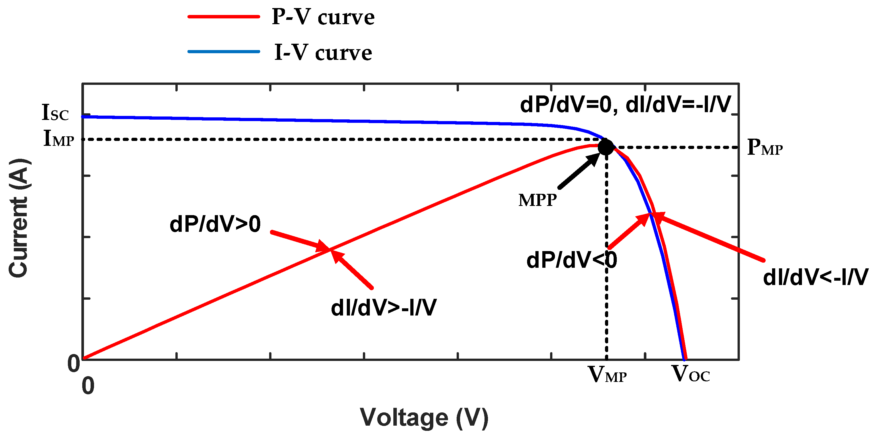
3.2. On-Line MPPT Techniques

Generally, the instantaneous values of the PV attempt output voltage or current are used to generate the control signals in online MPPT systems. A modest, methodical, and predetermined perturbation in the PV system’s voltage, current, or duty cycle is applied, together with the generated control signal, to determine the output power. The direction of change (increase or decrease) in the control signal is determined by analyzing how the PV panel’s output power responds to perturbation. These MPPT methods track MPP without any prior empirical information. Additionally, these methods are precise at varying temperatures and irradiances. Hill-climbing (HC), perturb and observe (P&O), and incremental conductance (IC) approaches are just a few of the MPPT methods that fall under this category [102].

P&O is the most widely used MPPT technique due to its simplicity and convenience in implementation [103,104]. In this technique, the output voltage of the PV panel is measured and perturbed by a small change, which causes a change in power (ΔP), as provided in Table 2. According to Table 2, the P&O technique works by perturbing the PV operating voltage decrease and increase, as shown in Figure 8. For every perturbing cycle, the PV output power is measured and compared. Through the perturbation process, the following can be noted:

If ∆P = 0, the system is working at the MPP and the voltage for the next sample remains constant.

If ∆P > 0 and ∆V > 0, then an increment is added to the operating voltage value to approach the MPP.

If ∆P > 0 and ∆V < 0, then the decrement is added to the operating voltage value to approach the MPP.

If ∆P < 0 and ∆V > 0, then the decrement is added to the operating voltage value to approach the MPP.

If ∆P < 0 and ∆V < 0, then an increment is added to the operating voltage value to approach the MPP.

Figure 8. P-V curve with P&O operating principle.

Figure 8. P-V curve with P&O operating principle.

Table 2. Perturb and observe methodology.

Perturbation (∆V)	Change in Power (∆P)	Next Perturbation Direction
∆V > 0 (Positive)	∆P > 0 (Positive)	Positive
∆V < 0 (Negative)	∆P > 0 (Positive)	Negative
∆V > 0 (Positive)	∆P < 0 (Negative)	Negative
∆V < 0 (Negative)	∆P < 0 (Negative)	Positive

Table 2. Perturb and observe methodology.

Perturbation (∆V)	Change in Power (∆P)	Next Perturbation Direction
∆V > 0 (Positive)	∆P > 0 (Positive)	Positive
∆V < 0 (Negative)	∆P > 0 (Positive)	Negative
∆V > 0 (Positive)	∆P < 0 (Negative)	Negative
∆V < 0 (Negative)	∆P < 0 (Negative)	Positive

In the P&O algorithm, a constant steady-state oscillation occurs at MPP, since the perturbations continuously change direction to retain the MPP under quickly varying solar irradiance, which decreases system efficiency and raises the losses in output power [103].

In terms of operating theory, the hill climbing (HC) technique is similar to the P&O approach; the only difference is the perturbation parameter. For MPP tracking, the P&O senses and perturbs the current or voltage, whereas the HC perturbs the duty cycle [21]. The output trade-off between the dynamic and steady-state response error is a common issue in both methods. This issue is more serious in the HC method, since it controls the duty cycle instead of voltage, while in the P and O method, voltage is regulated directly. Furthermore, due to a constant duty cycle, the traditional HC approach fails to extract the MPP efficiently under changing climate conditions [21].

The slope of the PV curve is discovered using INC, which is driven by Equations (10)–(12). Equation (10) determines if the PV module’s operating point is at its MPP, as shown in Figure 9. On the other hand, Equations (11) and (12) operate at the right and left sides of the unique operating point on the PV curve, respectively, to achieve the MPP by varying the duty cycle of the INC algorithm presented in

Table 3. INC algorithm.

Mode	Perturbation	MPP Level	Status
Mode-I	$\frac{dP}{dV}=0 \frac{dI}{dV}=-\frac{I}{V}$	At MPP	Hold VPV = VMPP
Mode-II	$\frac{dP}{dV}>0 \frac{dI}{dV}>-\frac{I}{V}$	Left side of MPP	Increase the voltage until VPV = VMPP
Mode-III	$\frac{dP}{dV}<0 \frac{dI}{dV}<-\frac{I}{V}$	Right side of MPP	Decrease the voltage until VPV = VMPP

[22].

$$\frac{dI}{dV}=-\frac{I}{V}$$

(10)

$$\frac{dI}{dV}<-\frac{I}{V}$$

(11)

$$\frac{dI}{dV}>-\frac{I}{V}$$

(12)

The scheme that involves Equations (10)–(12) assumes the slope of the PV curve at MPP is equal to zero, as shown in Equation (13).

$$\frac{dP}{dV}=0$$

(13)

Consequently, Equation (13) can be rewritten as

$$\frac{dP}{dV}=\frac{d\left(I\times V\right)}{dV}=V\frac{dI}{dV}+I\frac{dV}{dV}$$

(14)

$$\frac{dP}{dV}=V\frac{dI}{dV}+I$$

(15)

This implies that

$$\frac{dI}{dV}+\frac{I}{V}=0$$

(16)

One of the most often employed MPPT strategies is INC, along with P&O [22]. Nevertheless, in INC, the slope of the PV curve affects the duty cycle in either fixed or variable step sizes until the MPP is reached. These MPPT approaches employ a set step size, unlike the INC, HC, and P&O methods, whose process is dependent on the reference voltage’s step size. The controller can quickly reach the MPP with large steady-state oscillations by using a large step size. If not, reduced steady-state oscillations will occur with moderate convergence speeds for small step sizes, while the MPP for rapidly varying irradiance will be lost. Due to this, many modifications to the P&O MPPT method based on the P-V curve have been presented. However, they are thought to provide insufficient solutions for dealing with these issues.

K. M. Tsang et al. [105] presented the current sweep (CS) method based on MPPT for the PV system. The I-V curve of the module/panel is drawn using the module’s established operating conditions in the current sweep method. This approach extracts the current and voltage and manipulates them as a fixed function of time, as expressed in Equation (17).

𝑖 (𝑡) = 𝑓 (𝑡)

(17)

Since the current sweep method deals with the PV current and interprets the PV system’s I-V curve to evaluate the MPP, the MPP tracking cannot be achieved continuously. This approach is only used when the change in the calculated power is greater than a fixed threshold, which would be between 5% and 10% of the PV system’s maximum power. The meaning of the threshold cannot be too high or low. The current sweeping would be rarely performed if the threshold is set too high. The current sweeping would be near-continuous if the current is too minimal. Until the next current sweep, when the new MPP is calculated, the current sweep controller keeps the calculated voltage as the PV panel operating voltage [105].

The online methods also include the extremum seeking control (ESC) method and ripple correlation control (RCC) method. Bazzi and Krein [106], Brunton et al. [107] and Her-Terng and Chen [108] presented ESC methods to track the MPP. This method estimates MPP based on changes in the converter circuit’s current ripple and output power ripple. The PV system receives the reference current along with sinusoidal current perturbation. The PV system provides the output power ripple and the corresponding current ripple. If the current ripple is in the phase with the output power ripple, the MPP controller raises the ripple reference current to achieve I_MPP, and vice versa.

Kimball and Krein [109] proposed the ripple correlation control (RCC) method for extracting the MPP of the P-V curve of the PV system. The RCC technique is also similar to the ESC technique. To track the MPP, RCC uses the ripple imposed by the power converter on the PV array. It correlates dp/dt to dv/dt or di/dt to make the power gradient to zero, which occurs when the MPP is reached.

The RCC and ESC methods require the knowledge of the phase relationship between the dc power ripple and dc voltage or dc current ripple to determine the MPP. These methods are capable of achieving assured MPP. However, the practical implementation of these methods is very complex.

The authors have worked hard over the past ten years to improve global MPP monitoring by altering the traditional P&O and INC approaches. However, these modified classical approaches can result in power loss at the local MPP, due to rapidly varying shade conditions. The MPP of the PV system can be extracted using the sliding mode control (SMC) approach, according to the authors. The best choice of sliding surface is crucial to this method’s success. The sliding surface’s incorrect design produces an undesirable value. As a result, choosing the best sliding surfaces is a challenging task.

The advantages of online MPPT techniques are that they are simple and fast-tracking techniques. The disadvantages of online MPPT methods are as follows:

Undesired oscillations around MPP.

May not distinguish between global maxima, cluster head maxima, and local maxima.

Under partial shading, the power loss is very high.

Accuracy depends on the magnitude of the perturbation.

A comparison of various online MPPT techniques is presented in

Table 4. A comparison of various online MPPT techniques.

MPPT Technique	PV Array Dependency	Control Variable		Circuitry		Parameter Tuning	Tracking Accuracy	Efficiency	Complexity
		V	I	A	D
P&O	No	✓	✓	✓	✓	No	Moderate	High	Simple
INC	No	✓	✓		✓	No	High	High	Complex
HC	No	✓	✓	✓	✓	No	Moderate	High	Simple
CS	Yes	✓	✓	✓	✓	Yes	Medium	Medium	Complex
ESC	No	✓	✓	✓	✓	No	High	High	Medium
RCC	No	✓	✓	✓		Yes	Moderate	High	Complex
SMC	No	✓	✓		✓	No	Medium	High	Complex

.

3.3. Intelligent MPPT Techniques

Since conventional MPPT procedures are ineffective and prone to being caught between LMPPs, successfully tracking the GMPP in bad weather is a significant issue. The use of intelligent techniques is one viable way to measure GMPP under non-uniform sun irradiation and partial shading. The intelligent MPPT techniques include both artificial evolutionary algorithms. The MPPT techniques that belong to this category include, but are not limited to, the FLC, ANN, PSO, GWO, GO, and Jaya algorithm (JAYA), etc. To address the aforementioned issue, intelligent MPPT methods are used under non-uniform and shadowed solar conditions.

3.3.1. Fuzzy Logic Control (FLC)

The FLC is a robust approach for solving non-linear optimization problems. The fuzzy approach is preferred in MPPT implementation due to advantages such as (i) convenient user interface, (ii) ease of implementation, (iii) flexible operation, and (iv) qualified validation. However, FLC is rarely employed alone; although, it is extremely useful when combined with other algorithms, such as artificial neural networks [35], genetic algorithms, and other traditional methods [110,111]. For MPP tracking, the FLC approach uses three steps, fuzzification, inference fuzzy rules, and defuzzification. The optimal performance of the system is determined through fuzzy inference and fuzzy rule creation in these processes. However, to build fuzzy rules, a significant amount of information and training is required [38].

The FLC MPPT uses two inputs and one output for extracting maximum power from the PV system. The input variables are errors and change in errors, as presented in Equations (18) and (19), and the output variable is change in duty, as presented in Equation (20).

$$E\left(k\right)=\frac{∆P}{∆V}=\frac{P\left(k\right)-P\left(k-1\right)}{V\left(k\right)-V\left(k-1\right)}$$

(18)

$$∆E\left(k\right)=e\left(k\right)-e\left(k-1\right)$$

(19)

$$∆D=D\left(k\right)-D\left(k-1\right)$$

(20)

where

• E(k) represents the change in slope of the P-V curve;
• ∆e(k) denotes the change in the value of the slope of the P-V curve;
• ∆D denotes the change in the duty cycle.

The membership functions (MFs) of FLC for the input and output variables are presented in Figure 10. For input and output variables, the following five MFs are employed: big positive (BP), small positive (SP), zero (ZE), small negative (SN), and big negative (BN). The rule base of FLC presented in

Table 5. Fuzzy rule base.

		ΔE
		BN	SN	ZE	SP	BP
E	BN	ZE	ZE	ZE	BN	SP
	SN	ZE	ZE	SN	SN	SN
	ZE	SN	ZE	ZE	ZE	SP
	SP	SP	SP	SP	ZE	ZE
	BP	BP	BP	BP	ZE	ZE

is used to decrease the steady-state oscillations and to track MPP with fast tracking speed.

3.3.2. Artificial Neural Network

The term “artificial neural network” refers to a technique derived from the behavior of neurons. Because it is an artificial intelligence algorithm, ANN can think for itself. However, extensive knowledge is required to train the neurons [35,36,37]. According to the results of the survey, in the implementation of MPPT, ANN incorporates three layers. Figure 11 depicts a typical three-layer ANN model. Because of its broader optimization scope, the ANN is preferred for use in conjunction with other traditional MPPT methods to extract the most power from the PV system.

M. Sheraz and M. A. Abido [112] introduced a neural network to extract the MPP of PV modules and the design of a proportional integral-type controller for real-time optimum power tracking. The proposed neural network and the open circuit voltage applied by the regulating cells can be used to identify MPP. The suggested neural network created a PV module-based real-time MPP calculation. In comparison to straightforward mathematical calculation techniques, neural networks generally present a clearer image of functions. In contrast, a neural network works with random data without human intervention. As a result, it is highly dependent on the amount of data available to analyze the network, which makes it a laborious and complicated process. So, as a last resort to deal with issues relating to a lack of competence, neural network analysis is used.

The third group includes artificial intelligence methods, such as planning and neural networks, as well as fuzzy logic [37,112]. Studies have suggested using neural networks and fuzzy logic MPPT to address the shortcomings of traditional approaches, which has led to their increased popularity. Since the PV module’s features must be provided in order to create MPPT control rules, these solutions, however, are limited in their flexibility. FLCs are commonly employed in MPPT because of their many benefits, including their ability to work with wrong inputs, resolve nonlinearity, and not need a proper mathematical model. Additionally, the FLCs are unaffected by changes in environmental conditions. However, the user must choose an acceptable method for calculating the error and formulate the table of base rules to ensure that they are accurate, and FLCs require a significant amount of memory to handle the two extremes.

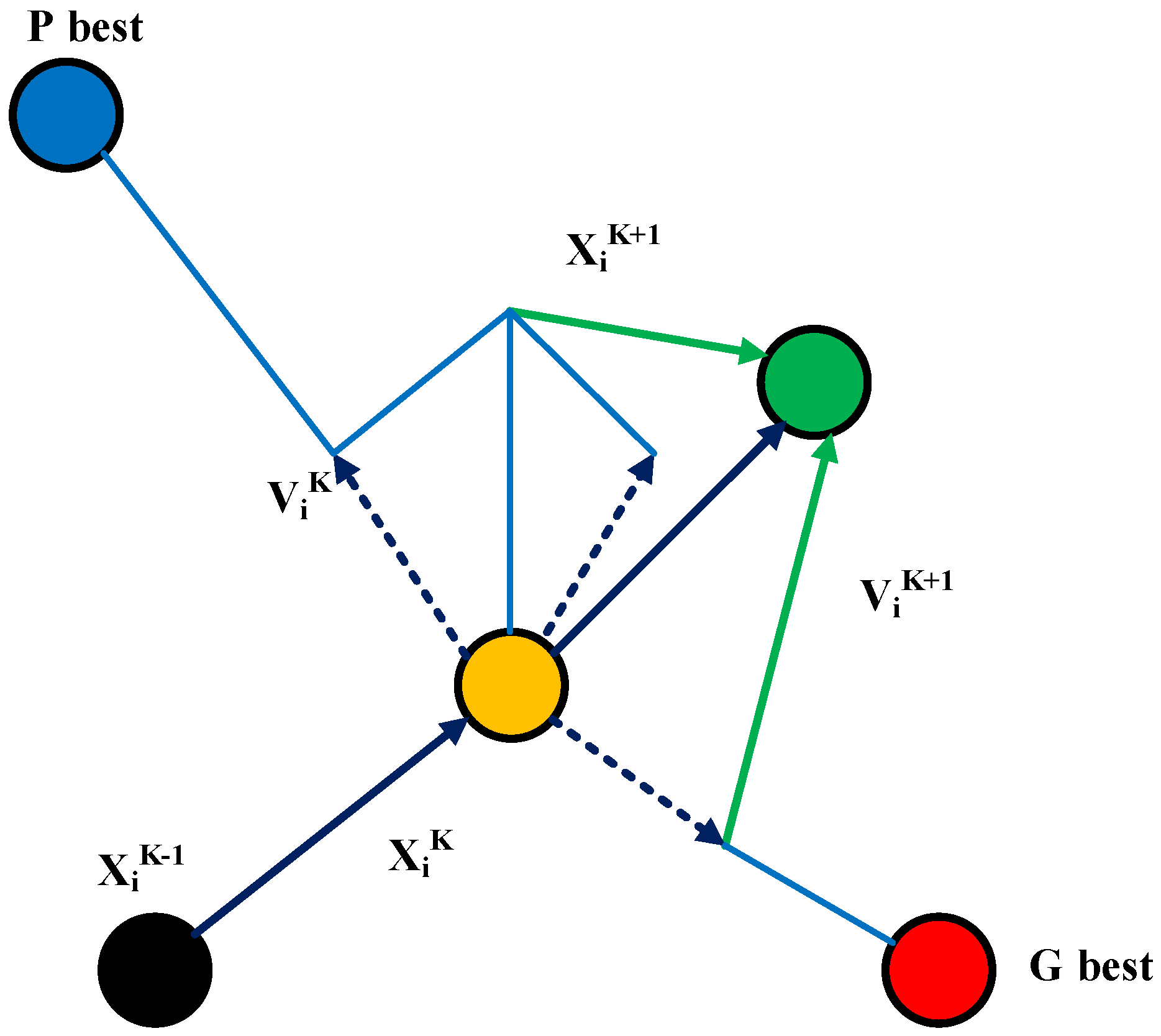
3.3.3. Particle Swarm Optimization

To address the aforementioned issue, swarm intelligence and bio-inspired approaches are applied in PVS for extracting maximum power (global peak) from the P-V curve. The application of swarm methods significantly increased interest in PVS research and effectively solved the issue of global MPP extraction. Typically, ant colonies, flocks of birds, and schools of fish served as the inspiration for swarm intelligence algorithms [46,47,48,49,50]. The three main benefits of these strategies are that they are simple to implement, begin with a random search, and prevent convergence to local minima.

The ability of the PSO algorithm has made it the best optimal optimization for nonlinear problems. The PSO algorithm derives its searchability from the behavior of flocks and swarms [50]. PSO has become one of the most popular optimization techniques for MPPT applications over the last decade. The fundamental concept of PSO is that the particles’ initial values are randomly chosen within the boundary limits. These particles (duty cycles) are programmed to move around in the search space. The best particle movement in the initial values is referred to as Pbest, and the overall best in subsequent iterations is referred to as Gbest. Furthermore, the particles’ position and velocity are updated with each iteration, and the process is repeated until the best position is found. The particle movement in search space is presented in Figure 12.

A particle status on the search space is characterized by the following two factors:

– Its velocity position (V_i);

– Position (X_i).

This will be updated according to the following equations:

$$V_i\left(k+1\right)=W{V}_i\left(k\right)+C_{1}ran{d}_1\ast \left(Pbes{t}_i\left(k\right)-X_i\left(k\right)\right)+C_{2}ran{d}_2\ast (Gbes{t}_i\left(k\right)-X_i\left(k\right))$$

(21)

$$X_i\left(k+1\right)=X_i\left(k\right)+V_i\left(k+1\right)$$

(22)

${\mathit{X}}_{\mathit{i}}\left(\mathit{k}+\mathbf{1}\right)$is the particle position at k+1th iteration, ${\mathit{X}}_{\mathit{i}}\left(\mathit{k}\right)$ is the particle position at kth iteration, ${\mathit{V}}_{\mathit{i}}\left(\mathit{k}+1\right)$ is the particle velocity at k+1th iteration, ${\mathit{V}}_{\mathit{i}}\left(\mathit{k}\right)$ is the particle velocity at kth iteration,${\mathit{C}}_{\mathbf{1}}$ is the acceleration component associated with Gbest, ${\mathit{C}}_{\mathbf{2}}$ is the acceleration component associated with Lbest, W is the inertia weight, rand1 and rand2 are random numbers from 0 and 1, Gbest is the best position of all particles, and Pbest is the best position of the particle.

The PSO was the first swarm algorithm to be used in PV MPPT applications. However, as the randomness decreases, PSO loses its diversity. Additionally, because it depends on the starting position of the search agent, convergence is delayed [46,47,48,49,50,51,52]. Furthermore, if the initial duty cycle value is not chosen properly, the PSO approach may become caught at the local MPP under PSCs.

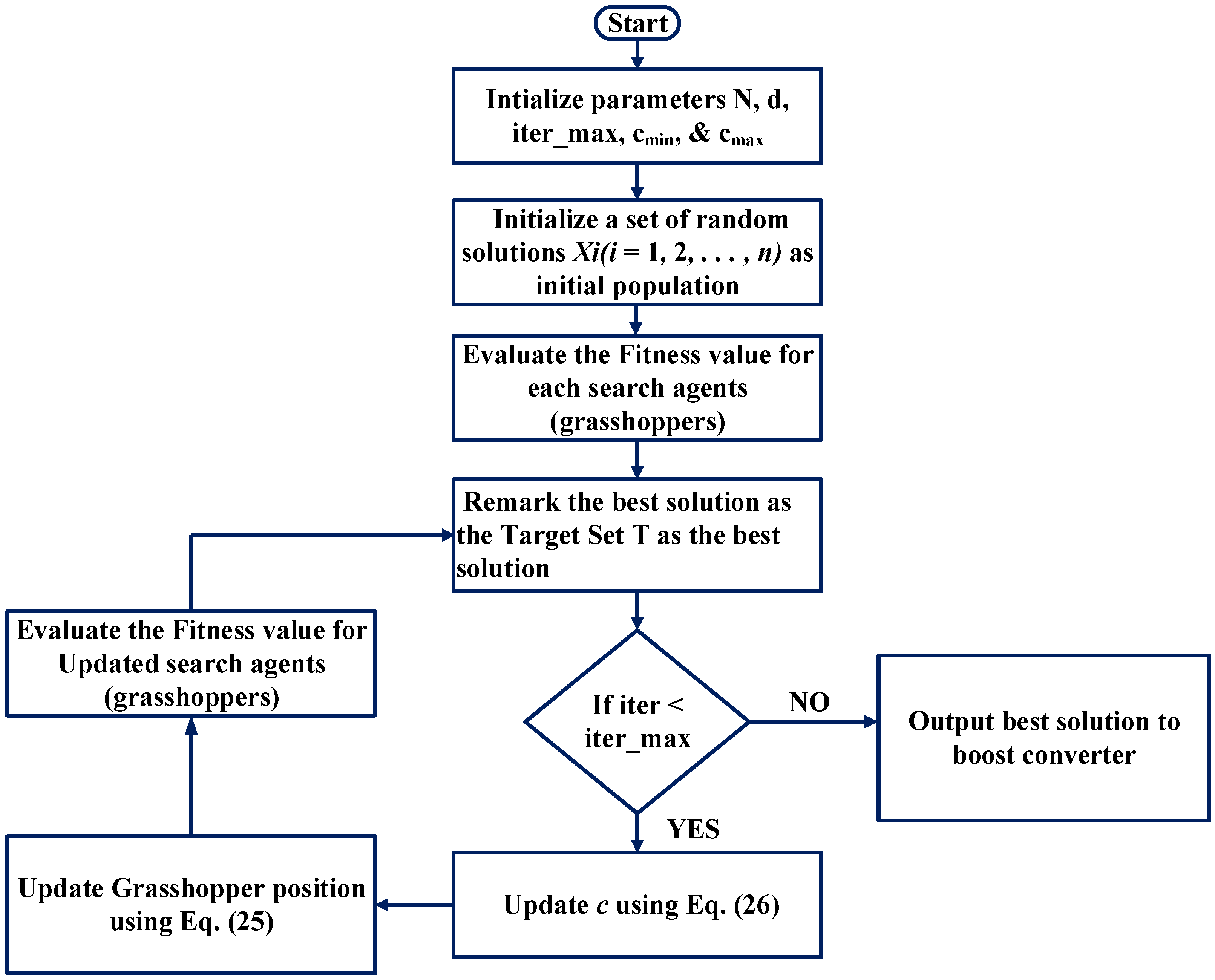
3.3.4. Grasshopper Optimization

The grasshopper optimization (GO) algorithm is a recently developed nature-inspired optimization technique based on how grasshoppers search for food [113]. The GO algorithm mimics the social interaction and behavior of grasshopper swarms. Grasshoppers are destructive insects due to the harm they cause to crops. Grasshoppers experience two swarm periods during their life cycle, the larval and adult phases. As larvae, grasshoppers walk slowly and eat every plant in their path. They grow wings and form swarms in the air when they are adults. The two stages of a grasshopper’s search for food are exploration and exploitation. During the exploration stage, the grasshoppers (search agents) move quickly, while during the exploitation stage, they are encouraged to move locally. The following is a summary of the mathematical modeling of grasshopper swarming behavior:

$$X_i=r_1{S}_i+r_2{G}_i+r_3{A}_i$$

(23)

where

X_i represents the position of the ith grasshopper, S_i is the social interaction of the ith grasshopper, G_i is the gravity force of the ith grasshopper, A_i is the wind advection of the ith grasshopper, and r_1, r₂, and r₃ are random numbers.

Therefore, using Equation (23), this can be expressed as the following using the elements S, G, and A:

$$X_i=r_1\left({\sum }_{\begin{array}{c}j=1\\ j\ne i\end{array}}^{N}S\left(\left|x_j-x_i\right|\right)\frac{x_j-x_i}{D_{ij}}\right)-r_{2}g\overrightarrow{e_g}+r_{3}u\overrightarrow{e_w}$$

(24)

where N indicates the number of grasshoppers (agents).

The Equation (24) can be adjusted as follows to converge to the specified point:

$$X^d{}_i=c\left({\sum }_{\begin{array}{c}j=1\\ j\ne i\end{array}}^{N}c\frac{u{b}_d-l{b}_d}{2}S\left(\left|x_j^d-x_i^d\right|\right)\frac{x_j-x_i}{D_{ij}}\right)+\overrightarrow{T_d}$$

(25)

where $\overrightarrow{T_d}$ denotes the target value (optimal solution) and $u{b}_d$, $l{b}_d$ denote the upper and lower bounds, respectively, c denotes the decreasing coefficients to reduce the comfort, repulsion, and attraction regions. Equation (26) can be used to update the coefficient c, increasing exploitation and decreasing exploration proportionally to iteration.

$$c=c_{max}-l\frac{c_{max}-c_{min}}{Iter\_max}$$

(26)

where l stands for the current iteration, $Iter\_max$ is the total number of iterations, and c min, $c_{min}$, $c_{max}$ are the minimum and maximum bounds of the decreasing coefficient. The GO method is applied to various engineering issues because of its significant advantages, including simplicity, quick convergence characteristics, an easy implementation structure, and a minimal number of regulating factors. Based on these advantages, the GO algorithm is employed in MPPT tracking of the solar PV system. The flowchart for the GO-based MPPT technique is shown in Figure 13.

GO is used to track GMPP because of its rapid convergence and its lowest number of oscillations when in a steady condition. The population is initially between 0 and 1 at random. The search space here stands for a boost converter duty cycle. The restrictions are adjusted suitably in the search space, where values range from 0 to 1. Every search agent in the GO algorithm provides a possible solution and the best solution (duty cycle) found so far is considered as the output of the MPPT technique. The position of every search agent in the GO represents the duty cycle and the value of the duty cycle can be updated using Equation (25).

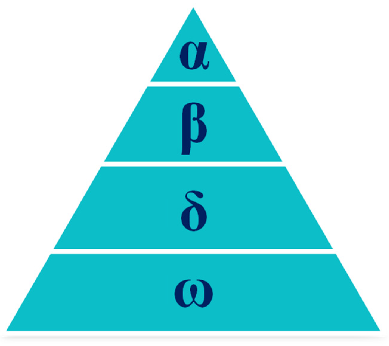
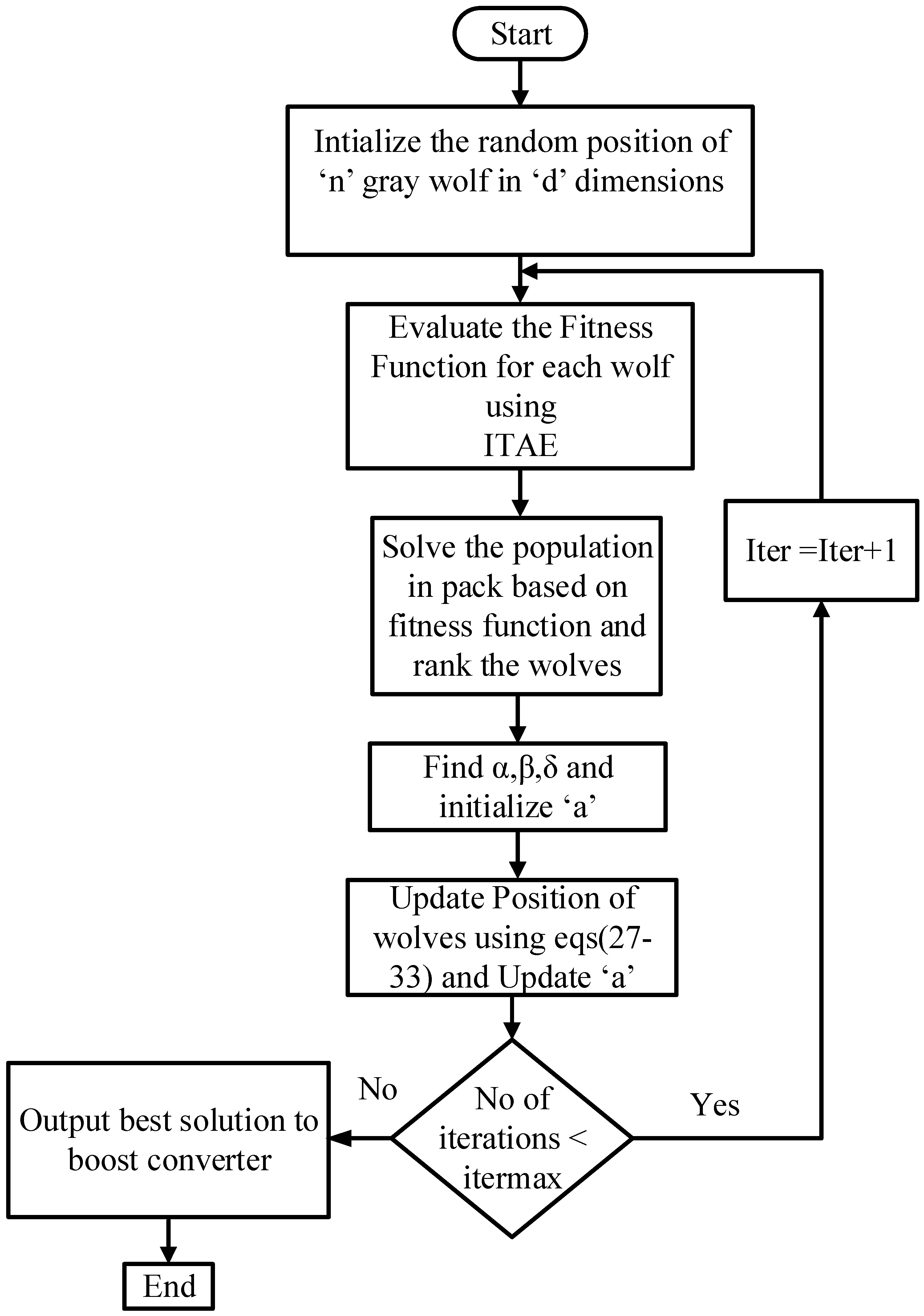
3.3.5. Grey Wolf Optimization

The GWO method is proposed to tackle the nonlinear problems based on the social behavior of grey wolves in nature [114]. As observed in Figure 14, grey wolves live in packs of 5 to 12 animals and have a clear dominating order. Based on their capacity to pursue prey, grey wolves are categorized into the following four groups: alpha, beta, delta, and omega. When creating the GWO algorithm, the alpha wolves are regarded as the best solution. As a result, beta wolves are the second best solution in the pack, and delta wolves are the third best. In the pack, the leftover wolves are classified as the omega category. The hunting behaviors of grey wolves, such as encircling, hunting, and attacking prey, are used to design the GWO algorithm for optimization problems. This hunting behavior can be expressed mathematically as follows:

$$\overrightarrow{D}=|\overrightarrow{C}.\overrightarrow{X_p^n}-\overrightarrow{X^n}|$$

(27)

$${\overrightarrow{X}}^{n+1}=\overrightarrow{X^n}+\overrightarrow{A}.\overrightarrow{D}$$

(28)

The coefficient vectors $\overrightarrow{A}$, $\overrightarrow{C}$ can be obtained as follows:

$$\overrightarrow{A}=2\overrightarrow{a}.{\overrightarrow{r}}_1-\overrightarrow{a}$$

(29)

$$\overrightarrow{C}=2.{\overrightarrow{r}}_2$$

(30)

where ${\overrightarrow{r}}_1,{\overrightarrow{r}}_2$ are the random numbers between 0 and 1, and $\overrightarrow{a}$ is linearly varied from 2 to 0. The hunt is typically led by alphas known as leaders, who are followed by betas and deltas who may hunt on occasion. The wounded wolves in the pack are cared for by delta and omega. As a result, we refer to alpha as the candidate solution that has a better understanding of the location of prey. When the prey stops moving, the grey wolves finish the hunt.

Grey wolves hunting behavior can be expressed as follows:

$${\overrightarrow{D}}_{\alpha }=\left|{\overrightarrow{C}}_1.{\overrightarrow{X}}_{\alpha }-\overrightarrow{X}\right|;{\overrightarrow{D}}_{\beta }=\left|{\overrightarrow{C}}_1.{\overrightarrow{X}}_{\beta }-\overrightarrow{X}\right|; {\overrightarrow{D}}_{\delta }=\left|{\overrightarrow{C}}_1.{\overrightarrow{X}}_{\delta }-\overrightarrow{X}\right|$$

(31)

$${\overrightarrow{X}}_1={\overrightarrow{X}}_{\alpha }-{\overrightarrow{A}}_1.\left({\overrightarrow{D}}_{\alpha }\right); {\overrightarrow{X}}_2={\overrightarrow{X}}_{\beta }-{\overrightarrow{A}}_2.\left({\overrightarrow{D}}_{\beta }\right);{\overrightarrow{X}}_3={\overrightarrow{X}}_{\delta }-{\overrightarrow{A}}_3.\left({\overrightarrow{D}}_{\delta }\right)$$

(32)

$${\overrightarrow{X}}^{n+1}=\frac{{\overrightarrow{X}}_1+{\overrightarrow{X}}_2+{\overrightarrow{X}}_3}{3}$$

(33)

The block diagram of the PV system with the MPPT technique is presented in Figure 6. The output power is calculated for each grey wolf, or duty ratio, once the Vpv and Ipv have been measured using sensors. The flow chart of GWO is presented in Figure 15.

The P-V curve is classified as having multiple peaks with several local peaks (LPs) and one global peak (GP) during partial shading. It is worth noting that once the wolves locate the MPP, their correlated coefficient vectors approach zero. The suggested method aims to combine GWO with direct duty-cycle control, i.e., the duty cycle is maintained at a constant value at the MPP, reducing the steady-state oscillations present in conventional MPPT techniques, and finally, power loss due to oscillation is reduced, leading to higher system efficiency. The GWO-based MPPT is implemented by defining duty cycle D as a grey wolf. Hence, equation (28) can be expressed as follows:

D_i (k + 1) = D_i(k) − A·D

(34)

As a result, the GWO algorithm’s fitness function is written as

P(d_i^k) > P(d_i^k−1)

(35)

where P stands for power, d for duty cycle, i for the current number of grey wolves, and k for the number of iterations.

3.3.6. Jaya Algorithm

Many researchers have proposed different swarm-intelligence techniques for MPPT applications in the literature [42,43,44,45,46,47,48,49,50,51,52,53,54,55,56,57,58,59,60,61,62,63,64,65]. However, the performance of the majority of these techniques is heavily reliant on algorithm-specific parameters. For instance, in the case of PSO, cognitive parameters (c1, c2) and inertia weight are required (w); in the case of GA, crossover, mutation, and parent selection are required. Similarly, other algorithms, such as the cuckoo search (CS), ACO, the Bat algorithm, ABC, the GWO, and so on, require parameter tuning. Incorrect parameter selection or tuning may result in a suboptimal solution. To address this issue, an algorithm-specific parameters-free technique called the Jaya algorithm (JA) is introduced.

R.V. Rao introduced the Jaya algorithm in 2016, which was inspired by humanoid or animal activities [115]. In many cases, all humans or animals in a population are biologically distinct. However, they are all inspired by the elite or firm members of the population and seek to distance themselves from the lazy or weak members of the population. Throughout this algorithm, a candidate solution moves away from the worst solution, while simultaneously moving towards the best solution by mimicking this nature. Because of its fast convergence and simplicity, this algorithm has been effectively used to solve a variety of engineering problems [116,117,118,119].

Let p represent the size of the population (m = 1, 2--p), n represent the number of variables (v = 1, 2--n) and ITAE (Equation (39)) represent the fitness function that needs to be minimized. The ITAE identifies the population’s best option as X_best and the population’s worst solution as X_worst. The value of the vth variable for the mth candidate in the ith iteration is given as X_v,m,i. Then, the updated value of each variable $X_{v,m,i}^{\prime }$ in the population can be obtained as follows:

$$X_{v,m,i}^{\prime }=X_{v,m,i}+r_1\ast \left(X_{v,best,i}-\left|X_{v,m,i}\right|\right)-r_2\ast \left(X_{v,worst,i}-\left|X_{v,m,i}\right|\right)$$

(36)

In Equation (36), all members of the population are always moving towards the best solution (‘+’ indication) and away from the worst solution (‘-’ indication). Furthermore, the equation shows that, unlike other algorithms, the proposed algorithm is not dependent on any algorithmic-specific parameters. The updated value of the population member (X (v,m,i)′) is accepted only if it is greater than the old value (X (v,m,i)). r₁ and r₂ are random numbers ranging from 0 to 1.

$$X_{v,m,i}^{\prime }=\{\begin{array}{l}{X}_{v,m,i}, ITAE\left(X_{v,m,i}\right)>ITAE\left(X_{v,m,i}^{\prime }\right)\\ X_{v,m,i}^{\prime }, Otherwise\end{array}$$

(37)

The objective function of the MPPT problem optimization is to maximize the power generated by the PV arrays, which can be expressed as (38). The particle solutions are regarded as the duty cycle D_i.

$$P\left(D_{i,j}^{k+1}\right)>P\left(D_{i,j}^k\right)$$

(38)

where P(D_i) represents the instantaneous power at the duty cycle D_i.

The fitness function to maximize the PV output power can be expressed as follows:

$$FF=Max\{\underset{0}{\overset{t_{sim}}{{\displaystyle \int }}}t\ast \left(V_{PV}\ast I_{PV}\right)\ast dt\}$$

(39)

To use the Jaya algorithm for solar MPPT application, the initial particle solutions D_i are generated, and then they are iteratively updated by taking the best and worst solutions into account. The flow chart of Jaya-based MPPT is presented in Figure 16. The mathematical equation for updating particle solutions is as follows:

$$D_{i,j}^{\prime }=D_{i,j}+r_1\ast \left(D_{i,best}-\left|D_{i,j}\right|\right)-r_2\ast \left(D_{i,worst}-\left|D_{i,j}\right|\right)$$

(40)

4. Discussions and Comparative Analysis

Many MPPT techniques can be found in the literature. This research conducted a comprehensive evaluation of the literature on MPPT approaches for both partial shade (non-uniform) and uniform irradiance. These techniques are divided into the following three categories: online, offline, and intelligent MPPT techniques. All the MPPT methods aim to optimize the output power of a PV system in an unrelated way. The following aspects are explored in this section: the GMPP tracking capability, convergence speed, complexity, and environmental change sensitivity.

4.1. Capability of Tracking GMPP

Due to the fact that the solar PV system does not receive uniform sun irradiance in very close sites in a short time, there is a possibility of partial shade due to unavoidable conditions. These conditions may be responsible for the formation of multiple peaks (LMPPs) on the I-V and P-V characteristics, which affects the MPPT’s tracking efficiency. The online and offline MPPT techniques are incapable of tracking the GMPP under partial shading conditions, whereas intelligent MPPT techniques are capable of tracking the GMPP under all abnormal conditions, such as uniform and nonuniform conditions.

4.2. Convergence Speed

An efficient MPPT technique must be able to converge to the required voltage and current with high speed and accuracy, regardless of whether the solar irradiance changes steadily or dramatically. When compared to intelligent MPPT techniques, the offline techniques convergence speed is fast but fails to track accurate MPP, whereas online techniques track MPP faster with constant oscillations, but converges to LMPP under partial shading conditions. The offline MPPT approaches never operate at accurate MPP, and hence are not suitable for efficient systems. The online MPPT techniques have high power losses under partial shading and accuracy is dependent on the size of perturbation. Furthermore, the intelligent techniques converge the GMPP under all abnormal conditions with negligible oscillation.

4.3. Complexity

The selection of an appropriate MPPT, keeping in mind its design complexity for a specific PV system, is regarded as one of the critical factors. The degree of accuracy with which the algorithm seeks for the real GMPP in the presence of several LMPPs determines the complexity of the MPPT approach. Otherwise, the PV system will not be able to capture the maximum solar energy. Moreover, the configuration and implementation of the MPPT are dependent on the user’s knowledge of the device, with one person being skilled in dealing with analog circuits, while the other prefers digital circuits. However, intelligent MPPT algorithms are implemented in digital form, which necessitates computer programming and software experts.

4.4. Sensitivity

A good MPPT technique must be sensitive enough to operate under all abnormal (uniform and nonuniform) conditions or atmospheric changes. It must be able to react quickly and track the GMPP of the specific PV system at the given condition. The comparative assessment of all the MPPT techniques is presented in

Table 6. A comparative assessment of MPPT techniques.

Type of MPPT Technique	Offline MPPT	Online MPPT	Intelligent MPPT
Tracking speed	High	High	Medium
Tracking accuracy	Less	Moderate	High
Tracking efficiency	Poor	Medium	Very good
Steady-state Oscillations	Less	High	Less
GMPPT tracking under PSC	Yes	No	Yes
Suitability for high-efficiency operations	No	Yes	Yes
Suitability for environmental changing conditions	No	No	Yes

.

The offline MPPT techniques track MPP under uniform irradiance with fast tracking speed and fewer oscillations. These methods fail to track the GMPP under PSCs. Moreover, they fail to track accurate MPP for uniform irradiance. The drawback of offline techniques is that they require pre-estimation of the parameters. Therefore, to overcome these issues, offline MPPT techniques must be combined with the heuristics techniques for tracking GMPP. Similarly, online techniques offer fast tracking speed, less steady state oscillations, and better tracking efficiency. However, these techniques fail to track GMPP under PSCs. Hence, they require modifications and/or to be combined with swam techniques. Unlike the offline and online MPPT methods, intelligent techniques track the GMPP under PSCs. The intelligent MPPT techniques improve tracking accuracy, tracking efficiency, steady state oscillations, and suitability with changing climatic conditions. However, the convergence speed of these techniques is less with high starting oscillations. Therefore, more research needs to be carried out to improve the convergence speed and reduce the starting oscillations.

The existing reviews provide the MPPT techniques based on uniform and partial shading conditions. They provided the details of a few conventional and swarm algorithm-based MPPT techniques. In addition, they performed a comparison of these techniques. The existing MPPT methods have drawbacks, such as being trapped at local MPP under PSCs, high initial oscillations, and slow tracking speed. Furthermore, to overcome these issues, hybrid intelligent MPPT techniques can be formed by combining the conventional and swarm algorithms or combining two heuristic methods.

5. Conclusions

Solar PV is regarded as the most promising energy source in the renewable energy generation system, due to the abundant availability of sunlight. However, it has some drawbacks, such as weather inconsistency, low efficiency, and high initial investment. As a result, MPPT is used as a power electronics interface to obtain the maximum power output of the PV system under both uniform and non-uniform shading conditions. So far, extensive research has been carried out on MPPT to improve the efficiency of PV systems under various weather conditions. However, selecting the appropriate MPPT for the specific PV system configurations and conditions has always been difficult. Therefore, this paper provides an accurate summary and a thorough review of various MPPT techniques. This research is based on the most commonly used techniques in recent years, which have been benchmarked in MPPT implementation. To summarize, a comparative study based on the sensor used, convergence speed, complexity, and application under dynamic weather conditions is briefly examined. After a thorough examination of all offline, online, and intelligent MPPT methods, it has been determined that the offline MPPT techniques achieve faster MPP, but fail to track the accurate MPP. The online MPPT techniques track the MPP fas6er with constant oscillations and fail to track GMPP under shading conditions. However, intelligent MPPT techniques track the GMPP quickly and accurately under partial shading and rapidly changing solar irradiance conditions. However, because they are complex algorithms, they are difficult to implement using embedded technologies.

References

1. Ahmed, M.; Abdelrahem, M.; Kennel, R. Highly Efficient and Robust Grid Connected Photovoltaic System Based Model Predictive Control with Kalman Filtering Capability. Sustainability 2020, 12, 4542. [Google Scholar] [CrossRef]
2. Kannan, N.; Vakeesan, D. Solar Energy for Future World: A Review. Renew. Sustain. Energy Rev. 2016, 62, 1092–1105. [Google Scholar] [CrossRef]
3. Bastidas-Rodriguez, J.D.; Franco, E.; Petrone, G.; Ramos-Paja, C.A.; Spagnuolo, G. Maximum Power Point Tracking Architectures for Photovoltaic Systems in Mismatching Conditions: A Review. IET Power Electron. 2014, 7, 1396–1413. [Google Scholar] [CrossRef]
4. Bhatnagar, P.; Nema, R.K. Maximum Power Point Tracking Control Techniques: State-of-the-Art in Photovoltaic Applications. Renew. Sustain. Energy Rev. 2013, 23, 224–241. [Google Scholar] [CrossRef]
5. Verma, D.; Nema, S.; Shandilya, A.M.; Dash, S.K. Maximum Power Point Tracking (MPPT) Techniques: Recapitulation in Solar Photovoltaic Systems. Renew. Sustain. Energy Rev. 2016, 54, 1018–1034. [Google Scholar] [CrossRef]
6. Reisi, A.R.; Moradi, M.H.; Jamasb, S. Classification and Comparison of Maximum Power Point Tracking Techniques for Photovoltaic System: A Review. Renew. Sustain. Energy Rev. 2013, 19, 433–443. [Google Scholar] [CrossRef]
7. Subudhi, B.; Pradhan, R. A Comparative Study on Maximum Power Point Tracking Techniques for Photovoltaic Power Systems. IEEE Trans. Sustain. Energy 2012, 4, 89–98. [Google Scholar] [CrossRef]
8. Kamarzaman, N.A.; Tan, C.W. A Comprehensive Review of Maximum Power Point Tracking Algorithms for Photovoltaic Systems. Renew. Sustain. Energy Rev. 2014, 37, 585–598. [Google Scholar] [CrossRef]
9. Koutroulis, E.; Blaabjerg, F. Overview of Maximum Power Point Tracking Techniques for Photovoltaic Energy Production Systems. In Renewable Energy Devices and Systems with Simulations in MATLAB® and ANSYS®; CRC Press: Boca Raton, FL, USA, 2017; pp. 91–130. [Google Scholar]
10. Ishaque, K.; Salam, Z. A Review of Maximum Power Point Tracking Techniques of PV System for Uniform Insolation and Partial Shading Condition. Renew. Sustain. Energy Rev. 2013, 19, 475–488. [Google Scholar] [CrossRef]
11. Lyden, S.; Haque, M.E. Maximum Power Point Tracking Techniques for Photovoltaic Systems: A Comprehensive Review and Comparative Analysis. Renew. Sustain. Energy Rev. 2015, 52, 1504–1518. [Google Scholar] [CrossRef]
12. Liu, Y.-H.; Chen, J.-H.; Huang, J.-W. A Review of Maximum Power Point Tracking Techniques for Use in Partially Shaded Conditions. Renew. Sustain. Energy Rev. 2015, 41, 436–453. [Google Scholar] [CrossRef]
13. Seyedmahmoudian, M.; Kok Soon, T.; Jamei, E.; Thirunavukkarasu, G.S.; Horan, B.; Mekhilef, S.; Stojcevski, A. Maximum Power Point Tracking for Photovoltaic Systems under Partial Shading Conditions Using Bat Algorithm. Sustainability 2018, 10, 1347. [Google Scholar] [CrossRef]
14. Salam, Z.; Ahmed, J.; Merugu, B.S. The Application of Soft Computing Methods for MPPT of PV System: A Technological and Status Review. Appl. Energy 2013, 107, 135–148. [Google Scholar] [CrossRef]
15. Kumar Dash, S.; Nema, S.; Nema, R.K.; Verma, D. A Comprehensive Assessment of Maximum Power Point Tracking Techniques under Uniform and Non-Uniform Irradiance and Its Impact on Photovoltaic Systems: A Review. J. Renew. Sustain. Energy 2015, 7, 063113. [Google Scholar] [CrossRef]
16. Sher, H.A.; Murtaza, A.F.; Noman, A.; Addoweesh, K.E.; Chiaberge, M. An Intelligent Control Strategy of Fractional Short Circuit Current Maximum Power Point Tracking Technique for Photovoltaic Applications. J. Renew. Sustain. Energy 2015, 7, 013114. [Google Scholar] [CrossRef]
17. Sher, H.A.; Murtaza, A.F.; Noman, A.; Addoweesh, K.E.; Al-Haddad, K.; Chiaberge, M. A New Sensorless Hybrid MPPT Algorithm Based on Fractional Short-Circuit Current Measurement and P&O MPPT. IEEE Trans. Sustain. Energy 2015, 6, 1426–1434. [Google Scholar]
18. Baimel, D.; Tapuchi, S.; Levron, Y.; Belikov, J. Improved Fractional Open Circuit Voltage MPPT Methods for PV Systems. Electronics 2019, 8, 321. [Google Scholar] [CrossRef]
19. Farayola, A.M.; Hasan, A.N.; Ali, A. Curve Fitting Polynomial Technique Compared to ANFIS Technique for Maximum Power Point Tracking. In Proceedings of the 2017 8th International Renewable Energy Congress (IREC), Amman, Jordan, 21–23 March 2017; pp. 1–6. [Google Scholar]
20. Lasheen, M.; Rahman, A.K.A.; Abdel-Salam, M.; Ookawara, S. Performance Enhancement of Constant Voltage Based MPPT for Photovoltaic Applications Using Genetic Algorithm. Energy Procedia 2016, 100, 217–222. [Google Scholar] [CrossRef]
21. Jately, V.; Azzopardi, B.; Joshi, J.; Sharma, A.; Arora, S. Experimental Analysis of Hill-Climbing MPPT Algorithms under Low Irradiance Levels. Renew. Sustain. Energy Rev. 2021, 150, 111467. [Google Scholar] [CrossRef]
22. Al-Dhaifallah, M.; Nassef, A.M.; Rezk, H.; Nisar, K.S. Optimal Parameter Design of Fractional Order Control Based INC-MPPT for PV System. Solar Energy 2018, 159, 650–664. [Google Scholar] [CrossRef]
23. Ferdous, S.M.; Shafiullah, G.M.; Oninda, M.A.M.; Shoeb, M.A.; Jamal, T. Close Loop Compensation Technique for High Performance MPPT Using Ripple Correlation Control. In Proceedings of the 2017 Australasian Universities Power Engineering Conference (AUPEC), Melbourne, VIC, Australia, 19–22 November 2017; pp. 1–6. [Google Scholar]
24. Femia, N.; Petrone, G.; Spagnuolo, G.; Vitelli, M. Optimization of Perturb and Observe Maximum Power Point Tracking Method. IEEE Trans. Power Electron. 2005, 20, 963–973. [Google Scholar] [CrossRef]
25. Pandey, A.; Dasgupta, N.; Mukerjee, A.K. High-Performance Algorithms for Drift Avoidance and Fast Tracking in Solar MPPT System. IEEE Trans. Energy Convers. 2008, 23, 681–689. [Google Scholar] [CrossRef]
26. Li, J.; Wang, H. A Novel Stand-Alone PV Generation System Based on Variable Step Size INC MPPT and SVPWM Control. In Proceedings of the 2009 IEEE 6th International Power Electronics and Motion Control Conference, Wuhan, China, 17–20 May 2009; pp. 2155–2160. [Google Scholar]
27. Liu, F.; Kang, Y.; Zhang, Y.; Duan, S. Comparison of P&O and Hill Climbing MPPT Methods for Grid-Connected PV Converter. In Proceedings of the 2008 3rd IEEE Conference on Industrial Electronics and Applications, Singapore, 3–5 June 2008; pp. 804–807. [Google Scholar]
28. Abdelsalam, A.K.; Massoud, A.M.; Ahmed, S.; Enjeti, P.N. High-Performance Adaptive Perturb and Observe MPPT Technique for Photovoltaic-Based Microgrids. IEEE Trans. Power Electron. 2011, 26, 1010–1021. [Google Scholar] [CrossRef]
29. Zainuri, M.A.A.M.; Radzi, M.A.M.; Che Soh, A.; Rahim, N.A. Development of Adaptive Perturb and Observe-Fuzzy Control Maximum Power Point Tracking for Photovoltaic Boost Dc–Dc Converter. IET Renew. Power Gener. 2014, 8, 183–194. [Google Scholar] [CrossRef]
30. Liu, F.; Duan, S.; Liu, F.; Liu, B.; Kang, Y. A Variable Step Size INC MPPT Method for PV Systems. IEEE Trans. Ind. Electron. 2008, 55, 2622–2628. [Google Scholar]
31. Xiao, W.; Dunford, W.G. A Modified Adaptive Hill Climbing MPPT Method for Photovoltaic Power Systems. In Proceedings of the 2004 IEEE 35th Annual Power Electronics Specialists Conference (IEEE Cat. No. 04CH37551), Aachen, Germany, 20–25 June 2004; Volume 3, pp. 1957–1963. [Google Scholar]
32. Ali, A.; Irshad, K.; Khan, M.; Hossain, M.; Al-Duais, I.; Malik, M. Artificial Intelligence and Bio-Inspired Soft Computing-Based Maximum Power Plant Tracking for a Solar Photovoltaic System under Non-Uniform Solar Irradiance Shading Conditions—A Review. Sustainability 2021, 13, 10575. [Google Scholar] [CrossRef]
33. Alaraj, M.; Kumar, A.; Alsaidan, I.; Rizwan, M.; Jamil, M. An Advanced and Robust Approach to Maximize Solar Photovoltaic Power Production. Sustainability 2022, 14, 7398. [Google Scholar] [CrossRef]
34. Ghazi, G.; Hasanien, H.; Al-Ammar, E.; Turky, R.; Ko, W.; Park, S.; Choi, H. African Vulture Optimization Algorithm-Based PI Controllers for Performance Enhancement of Hybrid Renewable-Energy Systems. Sustainability 2022, 14, 8172. [Google Scholar] [CrossRef]
35. Punitha, K.; Devaraj, D.; Sakthivel, S. Artificial Neural Network Based Modified Incremental Conductance Algorithm for Maximum Power Point Tracking in Photovoltaic System under Partial Shading Conditions. Energy 2013, 62, 330–340. [Google Scholar] [CrossRef]
36. Elobaid, L.M.; Abdelsalam, A.K.; Zakzouk, E.E. Artificial Neural Network-Based Photovoltaic Maximum Power Point Tracking Techniques: A Survey. IET Renew. Power Gener. 2015, 9, 1043–1063. [Google Scholar] [CrossRef]
37. Srinivasan, S.; Tiwari, R.; Krishnamoorthy, M.; Lalitha, M.P.; Raj, K.K. Neural Network Based MPPT Control with Reconfigured Quadratic Boost Converter for Fuel Cell Application. Int. J. Hydrog. Energy 2021, 46, 6709–6719. [Google Scholar] [CrossRef]
38. Liu, C.-L.; Chen, J.-H.; Liu, Y.-H.; Yang, Z.-Z. An Asymmetrical Fuzzy-Logic-Control-Based MPPT Algorithm for Photovoltaic Systems. Energies 2014, 7, 2177–2193. [Google Scholar] [CrossRef] [Green Version]
39. Tang, S.; Sun, Y.; Chen, Y.; Zhao, Y.; Yang, Y.; Szeto, W. An Enhanced MPPT Method Combining Fractional-Order and Fuzzy Logic Control. IEEE J. Photovolt. 2017, 7, 640–650. [Google Scholar] [CrossRef]
40. Aly, M.; Rezk, H. An Improved Fuzzy Logic Control-Based MPPT Method to Enhance the Performance of PEM Fuel Cell System. Neural Comput. Appl. 2022, 34, 4555–4566. [Google Scholar]
41. Cheng, P.-C.; Peng, B.-R.; Liu, Y.-H.; Cheng, Y.-S.; Huang, J.-W. Optimization of a Fuzzy-Logic-Control-Based MPPT Algorithm Using the Particle Swarm Optimization Technique. Energies 2015, 8, 5338–5360. [Google Scholar] [CrossRef]
42. González-Castaño, C.; Restrepo, C.; Kouro, S.; Rodriguez, J. MPPT Algorithm Based on Artificial Bee Colony for PV System. IEEE Access 2021, 9, 43121–43133. [Google Scholar] [CrossRef]
43. Soufyane Benyoucef, A.; Chouder, A.; Kara, K.; Silvestre, S. Artificial Bee Colony Based Algorithm for Maximum Power Point Tracking (MPPT) for PV Systems Operating under Partial Shaded Conditions. Appl. Soft Comput. 2015, 32, 38–48. [Google Scholar] [CrossRef]
44. Tajuddin, M.F.N.; Ayob, S.M.; Salam, Z.; Saad, M.S. Evolutionary Based Maximum Power Point Tracking Technique Using Differential Evolution Algorithm. Energy Build. 2013, 67, 245–252. [Google Scholar]
45. Ramasamy, S.; Dash, S.S.; Selvan, T. An Intelligent Differential Evolution Based Maximum Power Point Tracking (MPPT) Technique for Partially Shaded Photo Voltaic (PV) Array. Int. J. Adv. Soft Comput. Its Appl. 2014, 6, 1–16. [Google Scholar]
46. Koad, R.B.; Zobaa, A.F.; El-Shahat, A. A Novel MPPT Algorithm Based on Particle Swarm Optimization for Photovoltaic Systems. IEEE Trans. Sustain. Energy 2016, 8, 468–476. [Google Scholar] [CrossRef]
47. Khare, A.; Rangnekar, S. A Review of Particle Swarm Optimization and Its Applications in Solar Photovoltaic System. Appl. Soft Comput. 2013, 13, 2997–3006. [Google Scholar] [CrossRef]
48. Ishaque, K.; Salam, Z.; Amjad, M.; Mekhilef, S. An Improved Particle Swarm Optimization (PSO)–Based MPPT for PV with Reduced Steady-State Oscillation. IEEE Trans. Power Electron. 2012, 27, 3627–3638. [Google Scholar] [CrossRef]
49. Li, H.; Yang, D.; Su, W.; Lü, J.; Yu, X. An Overall Distribution Particle Swarm Optimization MPPT Algorithm for Photovoltaic System under Partial Shading. IEEE Trans. Ind. Electron. 2018, 66, 265–275. [Google Scholar] [CrossRef]
50. Sundareswaran, K.; Palani, S. Application of a Combined Particle Swarm Optimization and Perturb and Observe Method for MPPT in PV Systems under Partial Shading Conditions. Renew. Energy 2015, 75, 308–317. [Google Scholar] [CrossRef]
51. Luta, D.N.; Raji, A.K. Fuzzy Rule-Based and Particle Swarm Optimisation MPPT Techniques for a Fuel Cell Stack. Energies 2019, 12, 936. [Google Scholar] [CrossRef] [Green Version]
52. Jouda, A.; Elyes, F.; Rabhi, A.; Abdelkader, M. Optimization of Scaling Factors of Fuzzy–MPPT Controller for Stand-Alone Photovoltaic System by Particle Swarm Optimization. Energy Procedia 2017, 111, 954–963. [Google Scholar] [CrossRef]
53. Ahmed, J.; Salam, Z. A Maximum Power Point Tracking (MPPT) for PV System Using Cuckoo Search with Partial Shading Capability. Appl. Energy 2014, 119, 118–130. [Google Scholar]
54. Ahmed, J.; Salam, Z. A Soft Computing MPPT for PV System Based on Cuckoo Search Algorithm. In Proceedings of the 4th International Conference on Power Engineering, Energy and Electrical Drives, Istanbul, Turkey, 13–17 May 2013; pp. 558–562. [Google Scholar]
55. Kulaksız, A.A.; Akkaya, R. A Genetic Algorithm Optimized ANN-Based MPPT Algorithm for a Stand-Alone PV System with Induction Motor Drive. Sol. Energy 2012, 86, 2366–2375. [Google Scholar] [CrossRef]
56. Daraban, S.; Petreus, D.; Morel, C. A Novel MPPT (Maximum Power Point Tracking) Algorithm Based on a Modified Genetic Algorithm Specialized on Tracking the Global Maximum Power Point in Photovoltaic Systems Affected by Partial Shading. Energy 2014, 74, 374–388. [Google Scholar] [CrossRef]
57. Kumar, P.; Jain, G.; Palwalia, D.K. Genetic Algorithm Based Maximum Power Tracking in Solar Power Generation. In Proceedings of the 2015 International Conference on Power and Advanced Control Engineering (ICPACE), Bengaluru, India, 12–14 August 2015; pp. 1–6. [Google Scholar]
58. Hadji, S.; Gaubert, J.-P.; Krim, F. Real-Time Genetic Algorithms-Based MPPT: Study and Comparison (Theoretical an Experimental) with Conventional Methods. Energies 2018, 11, 459. [Google Scholar] [CrossRef]
59. Hadji, S.; Gaubert, J.-P.; Krim, F. Theoretical and Experimental Analysis of Genetic Algorithms Based MPPT for PV Systems. Energy Procedia 2015, 74, 772–787. [Google Scholar] [CrossRef]
60. Sundareswaran, K.; Peddapati, S.; Palani, S. MPPT of PV Systems under Partial Shaded Conditions through a Colony of Flashing Fireflies. IEEE Trans. Energy Convers. 2014, 29, 463–472. [Google Scholar]
61. Titri, S.; Larbes, C.; Toumi, K.Y.; Benatchba, K. A New MPPT Controller Based on the Ant Colony Optimization Algorithm for Photovoltaic Systems under Partial Shading Conditions. Appl. Soft Comput. 2017, 58, 465–479. [Google Scholar] [CrossRef]
62. Priyadarshi, N.; Ramachandaramurthy, V.K.; Padmanaban, S.; Azam, F. An Ant Colony Optimized MPPT for Standalone Hybrid PV-Wind Power System with Single Cuk Converter. Energies 2019, 12, 167. [Google Scholar] [CrossRef]
63. Zhou, L.; Chen, Y.; Liu, Q.; Wu, J. Maximum Power Point Tracking (MPPT) Control of a Photovoltaic System Based on Dual Carrier Chaotic Search. J. Control. Theory Appl. 2012, 10, 244–250. [Google Scholar]
64. Chen, M.; Ma, S.; Wu, J.; Huang, L. Analysis of MPPT Failure and Development of an Augmented Nonlinear Controller for MPPT of Photovoltaic Systems under Partial Shading Conditions. Appl. Sci. 2017, 7, 95. [Google Scholar] [CrossRef]
65. Sundareswaran, K.; Peddapati, S.; Palani, S. Application of Random Search Method for Maximum Power Point Tracking in Partially Shaded Photovoltaic Systems. IET Renew. Power Gener. 2014, 8, 670–678. [Google Scholar] [CrossRef]
66. Ramaprabha, R.; Balaji, M.; Mathur, B.L. Maximum Power Point Tracking of Partially Shaded Solar PV System Using Modified Fibonacci Search Method with Fuzzy Controller. Int. J. Electr. Power Energy Syst. 2012, 43, 754–765. [Google Scholar] [CrossRef]
67. Dallago, E.; Liberale, A.; Miotti, D.; Venchi, G. Direct MPPT Algorithm for PV Sources with Only Voltage Measurements. IEEE Trans. Power Electron. 2015, 30, 6742–6750. [Google Scholar] [CrossRef]
68. Pilakkat, D.; Kanthalakshmi, S. An Improved P&O Algorithm Integrated with Artificial Bee Colony for Photovoltaic Systems under Partial Shading Conditions. Sol. Energy 2019, 178, 37–47. [Google Scholar]
69. Ibnelouad, A.; El Kari, A.; Ayad, H.; Mjahed, M. Improved Cooperative Artificial Neural Network-Particle Swarm Optimization Approach for Solar Photovoltaic Systems Using Maximum Power Point Tracking. Int. Trans. Electr. Energy Syst. 2020, 30, e12439. [Google Scholar] [CrossRef]
70. Da Rocha, M.V.; Sampaio, L.P.; da Silva, S.A.O. Comparative Analysis of MPPT Algorithms Based on Bat Algorithm for PV Systems under Partial Shading Condition. Sustain. Energy Technol. Assess. 2020, 40, 100761. [Google Scholar] [CrossRef]
71. Guo, K.; Cui, L.; Mao, M.; Zhou, L.; Zhang, Q. An Improved Gray Wolf Optimizer MPPT Algorithm for PV System with BFBIC Converter under Partial Shading. IEEE Access 2020, 8, 103476–103490. [Google Scholar]
72. Khan, N.M.; Mansoor, M.; Mirza, A.F.; Moosavi, S.K.R.; Qadir, Z.; Zafar, M.H. Energy Harvesting and Stability Analysis of Centralized TEG System under Non-Uniform Temperature Distribution. Sustain. Energy Technol. Assess. 2022, 52, 102028. [Google Scholar]
73. Ram, J.P.; Babu, T.S.; Rajasekar, N. A Comprehensive Review on Solar PV Maximum Power Point Tracking Techniques. Renew. Sustain. Energy Rev. 2017, 67, 826–847. [Google Scholar]
74. Bollipo, R.B.; Mikkili, S.; Bonthagorla, P.K. Critical Review on PV MPPT Techniques: Classical, Intelligent and Optimisation. IET Renew. Power Gener. 2020, 14, 1433–1452. [Google Scholar]
75. Pathy, S.; Subramani, C.; Sridhar, R.; Thamizh Thentral, T.M.; Padmanaban, S. Nature-Inspired MPPT Algorithms for Partially Shaded PV Systems: A Comparative Study. Energies 2019, 12, 1451. [Google Scholar] [CrossRef]
76. Ali, A.; Almutairi, K.; Malik, M.Z.; Irshad, K.; Tirth, V.; Algarni, S.; Zahir, M.H.; Islam, S.; Shafiullah, M.; Shukla, N.K. Review of Online and Soft Computing Maximum Power Point Tracking Techniques under Non-Uniform Solar Irradiation Conditions. Energies 2020, 13, 3256. [Google Scholar] [CrossRef]
77. Derbeli, M.; Napole, C.; Barambones, O.; Sanchez, J.; Calvo, I.; Fernández-Bustamante, P. Maximum Power Point Tracking Techniques for Photovoltaic Panel: A Review and Experimental Applications. Energies 2021, 14, 7806. [Google Scholar] [CrossRef]
78. Laxman, B.; Annamraju, A.; Srikanth, N.V. A Grey Wolf Optimized Fuzzy Logic Based MPPT for Shaded Solar Photovoltaic Systems in Microgrids. Int. J. Hydrog. Energy 2021, 46, 10653–10665. [Google Scholar]
79. Gao, L.; Dougal, R.A.; Liu, S.; Iotova, A.P. Parallel-Connected Solar PV System to Address Partial and Rapidly Fluctuating Shadow Conditions. IEEE Trans. Ind. Electron. 2009, 56, 1548–1556. [Google Scholar]
80. Hashim, N.; Salam, Z. Critical Evaluation of Soft Computing Methods for Maximum Power Point Tracking Algorithms of Photovoltaic Systems. Int. J. Power Electron. Drive Syst. 2019, 10, 548. [Google Scholar] [CrossRef]
81. Verma, D.; Nema, S.; Shandilya, A.M.; Dash, S.K. Comprehensive Analysis of Maximum Power Point Tracking Techniques in Solar Photovoltaic Systems under Uniform Insolation and Partial Shaded Condition. J. Renew. Sustain. Energy 2015, 7, 042701. [Google Scholar] [CrossRef]
82. Yan, K.; Shen, H.; Wang, L.; Zhou, H.; Xu, M.; Mo, Y. Short-Term Solar Irradiance Forecasting Based on a Hybrid Deep Learning Methodology. Information 2020, 11, 32. [Google Scholar] [CrossRef]
83. Santana, E.; Silva, R.; Zarpelão, B.; Barbon Junior, S. Detecting and Mitigating Adversarial Examples in Regression Tasks: A Photovoltaic Power Generation Forecasting Case Study. Information 2021, 12, 394. [Google Scholar] [CrossRef]
84. Hajiabadi, M.; Farhadi, M.; Babaiyan, V.; Estebsari, A. Deep Learning with Loss Ensembles for Solar Power Prediction in Smart Cities. Smart Cities 2020, 3, 842–852. [Google Scholar] [CrossRef]
85. Pinna, A.; Massidda, L. A Procedure for Complete Census Estimation of Rooftop Photovoltaic Potential in Urban Areas. Smart Cities 2020, 3, 873–893. [Google Scholar] [CrossRef]
86. Rajalakshmi, M.; Chandramohan, S.; Kannadasan, R.; Alsharif, M.H.; Kim, M.-K.; Nebhen, J. Design and Validation of BAT Algorithm-Based Photovoltaic System Using Simplified High Gain Quasi Boost Inverter. Energies 2021, 14, 1086. [Google Scholar] [CrossRef]
87. Alturki, F.A.; Al-Shamma’a, A.; MH Farh, H. Simulations and dSPACE Real-Time Implementation of Photovoltaic Global Maximum Power Extraction under Partial Shading. Sustainability 2020, 12, 3652. [Google Scholar] [CrossRef]
88. Almutairi, A.; Abo-Khalil, A.; Sayed, K.; Albagami, N. MPPT for a PV Grid-Connected System to Improve Efficiency under Partial Shading Conditions. Sustainability 2020, 12, 10310. [Google Scholar] [CrossRef]
89. Islam, H.; Mekhilef, S.; Shah, N.; Soon, T.; Wahyudie, A.; Ahmed, M. Improved Proportional-Integral Coordinated MPPT Controller with Fast Tracking Speed for Grid-Tied PV Systems under Partially Shaded Conditions. Sustainability 2021, 13, 830. [Google Scholar] [CrossRef]
90. Pandiyan, P.; Saravanan, S.; Prabaharan, N.; Tiwari, R.; Chinnadurai, T.; Babu, N.; Hossain, E. Implementation of Different MPPT Techniques in Solar PV Tree under Partial Shading Conditions. Sustainability 2021, 13, 7208. [Google Scholar] [CrossRef]
91. Nagadurga, T.; Narasimham, P.; Vakula, V. Global Maximum Power Point Tracking of Solar Photovoltaic Strings under Partial Shading Conditions Using Cat Swarm Optimization Technique. Sustainability 2021, 13, 11106. [Google Scholar] [CrossRef]
92. Bindi, M.; Corti, F.; Aizenberg, I.; Grasso, F.; Lozito, G.; Luchetta, A.; Piccirilli, M.; Reatti, A. Machine Learning-Based Monitoring of DC-DC Converters in Photovoltaic Applications. Algorithms 2022, 15, 74. [Google Scholar] [CrossRef]
93. Alaraj, M.; Dube, A.; Alsaidan, I.; Rizwan, M.; Jamil, M. Design and Development of a Proficient Converter for Solar Photovoltaic Based Sustainable Power Generating System. Sustainability 2021, 13, 2045. [Google Scholar] [CrossRef]
94. Kanagaraj, N. Photovoltaic and Thermoelectric Generator Combined Hybrid Energy System with an Enhanced Maximum Power Point Tracking Technique for Higher Energy Conversion Efficiency. Sustainability 2021, 13, 3144. [Google Scholar] [CrossRef]
95. Kedika, N.R.; Bhukya, L.; Punna, S.; Motamarri, R. Single-Phase Seven-Level Inverter with Multilevel Boost Converter for Solar Photovoltaic Systems. In Proceedings of the 2022 Second International Conference on Power, Control and Computing Technologies (ICPC2T), Raipur, India, 1–3 March 2022; pp. 1–6. [Google Scholar]
96. Vitorino, M.A.; Hartmann, L.V.; Lima, A.M.; Corrêa, M.B. Using the Model of the Solar Cell for Determining the Maximum Power Point of Photovoltaic Systems. In Proceedings of the 2007 European Conference on Power Electronics and Applications, Aalborg, Denmark, 2–5 September 2007; pp. 1–10. [Google Scholar]
97. Ali, A.; Almutairi, K.; Padmanaban, S.; Tirth, V.; Algarni, S.; Irshad, K.; Islam, S.; Zahir, M.H.; Shafiullah, M.; Malik, M.Z. Investigation of MPPT Techniques under Uniform and Non-Uniform Solar Irradiation Condition–a Retrospection. IEEE Access 2020, 8, 127368–127392. [Google Scholar] [CrossRef]
98. Fapi, C.B.N.; Wira, P.; Kamta, M.; Tchakounté, H.; Colicchio, B. Simulation and DSPACE Hardware Implementation of an Improved Fractional Short-Circuit Current MPPT Algorithm for Photovoltaic System. Appl. Sol. Energy 2021, 57, 93–106. [Google Scholar]
99. Bu, L.; Quan, S.; Han, J.; Li, F.; Li, Q.; Wang, X. On-Site Traversal Fractional Open Circuit Voltage with Uninterrupted Output Power for Maximal Power Point Tracking of Photovoltaic Systems. Electronics 2020, 9, 1802. [Google Scholar] [CrossRef]
100. Salas, V.; Olias, E.; Barrado, A.; Lazaro, A. Review of the Maximum Power Point Tracking Algorithms for Stand-Alone Photovoltaic Systems. Sol. Energy Mater. Sol. Cells 2006, 90, 1555–1578. [Google Scholar] [CrossRef]
101. Yilmaz, U.; Kircay, A.; Borekci, S. PV System Fuzzy Logic MPPT Method and PI Control as a Charge Controller. Renew. Sustain. Energy Rev. 2018, 81, 994–1001. [Google Scholar] [CrossRef]
102. Safari, A.; Mekhilef, S. Simulation and Hardware Implementation of Incremental Conductance MPPT with Direct Control Method Using Cuk Converter. IEEE Trans. Ind. Electron. 2010, 58, 1154–1161. [Google Scholar] [CrossRef]
103. Femia, N.; Petrone, G.; Spagnuolo, G.; Vitelli, M. A Technique for Improving P&O MPPT Performances of Double-Stage Grid-Connected Photovoltaic Systems. IEEE Trans. Ind. Electron. 2009, 56, 4473–4482. [Google Scholar]
104. Ahmed, J.; Salam, Z. An Enhanced Adaptive P&O MPPT for Fast and Efficient Tracking under Varying Environmental Conditions. IEEE Trans. Sustain. Energy 2018, 9, 1487–1496. [Google Scholar]
105. Tsang, K.M.; Chan, W.L. Maximum Power Point Tracking for PV Systems under Partial Shading Conditions Using Current Sweeping. Energy Convers. Manag. 2015, 93, 249–258. [Google Scholar] [CrossRef]
106. Matsuura, M.; Nomoto, H.; Mamiya, H.; Higuchi, T.; Masson, D.; Fafard, S. Over 40-W Electric Power and Optical Data Transmission Using an Optical Fiber. IEEE Trans. Power Electron. 2020, 36, 4532–4539. [Google Scholar] [CrossRef]
107. Brunton, S.L.; Rowley, C.W.; Kulkarni, S.R.; Clarkson, C. Maximum Power Point Tracking for Photovoltaic Optimization Using Ripple-Based Extremum Seeking Control. IEEE Trans. Power Electron. 2010, 25, 2531–2540. [Google Scholar] [CrossRef]
108. Yau, H.-T.; Wu, C.-H. Comparison of Extremum-Seeking Control Techniques for Maximum Power Point Tracking in Photovoltaic Systems. Energies 2011, 4, 2180–2195. [Google Scholar] [CrossRef]
109. Kimball, J.W.; Krein, P.T. Discrete-Time Ripple Correlation Control for Maximum Power Point Tracking. IEEE Trans. Power Electron. 2008, 23, 2353–2362. [Google Scholar] [CrossRef]
110. Shiau, J.; Wei, Y.; Chen, B. A Study on the Fuzzy-Logic-Based Solar Power MPPT Algorithms Using Different Fuzzy Input Variables. Algorithms 2015, 8, 100–127. [Google Scholar] [CrossRef]
111. Remoaldo, D.; Jesus, I. Analysis of a Traditional and a Fuzzy Logic Enhanced Perturb and Observe Algorithm for the MPPT of a Photovoltaic System. Algorithms 2021, 14, 24. [Google Scholar] [CrossRef]
112. Sheraz, M.; Abido, M.A. An Efficient MPPT Controller Using Differential Evolution and Neural Network. In Proceedings of the 2012 IEEE International Conference on Power and Energy (PECon), Kota Kinabalu, Malaysia, 2–5 December 2012; pp. 378–383. [Google Scholar]
113. Bhukya, L.; Nandiraju, S. A Novel Photovoltaic Maximum Power Point Tracking Technique Based on Grasshopper Optimized Fuzzy Logic Approach. Int. J. Hydrog. Energy 2020, 45, 9416–9427. [Google Scholar] [CrossRef]
114. Rezaei, H.; Bozorg-Haddad, O.; Chu, X. Grey Wolf Optimization (GWO) Algorithm. In Advanced Optimization by Nature-Inspired Algorithms; Springer: Berlin/Heidelberg, Germany, 2018; pp. 81–91. [Google Scholar]
115. Rao, R.V.; Saroj, A. A Self-Adaptive Multi-Population Based Jaya Algorithm for Engineering Optimization. Swarm Evol. Comput. 2017, 37, 1–26. [Google Scholar]
116. Rao, R.V.; More, K.; Taler, J.; Oc\loń, P. Dimensional Optimization of a Micro-Channel Heat Sink Using Jaya Algorithm. Appl. Therm. Eng. 2016, 103, 572–582. [Google Scholar] [CrossRef]
117. Warid, W.; Hizam, H.; Mariun, N.; Abdul-Wahab, N.I. Optimal Power Flow Using the Jaya Algorithm. Energies 2016, 9, 678. [Google Scholar] [CrossRef]
118. Bhukya, L.; Annamraju, A.; Nandiraju, S. A Novel Maximum Power Point Tracking Technique Based on Rao-1 Algorithm for Solar PV System under Partial Shading Conditions. Int. Trans. Electr. Energy Syst. 2021, 31, e13028. [Google Scholar] [CrossRef]
119. Rao, R.V.; Rai, D.P.; Balic, J. Surface Grinding Process Optimization Using Jaya Algorithm. In Computational Intelligence in Data Mining—Volume 2; Springer: Berlin/Heidelberg, Germany, 2016; pp. 487–495. [Google Scholar]
Figure 1. PV cell model.
Algorithms 15 00365 g001
Figure 2. From solar cell to array.
Algorithms 15 00365 g002
Figure 3. The I-V and P-V curves.
Algorithms 15 00365 g003
Figure 4. Solar PV Characteristics for (a) different values of irradiances and (b) different values of temperature.
Algorithms 15 00365 g004
Figure 5. The P-V curves under various shading conditions.
Algorithms 15 00365 g005
Figure 6. Block diagram representation of PV MPPT.
Algorithms 15 00365 g006
Figure 7. Classifications of MPPT techniques.
Algorithms 15 00365 g007
Figure 9. P-V curve of the PV system and signs of its slope at various regions.
Algorithms 15 00365 g009
Figure 10. (a) Input; (b) change in input and (c) output membership functions.
Algorithms 15 00365 g010
Figure 11. Three-layer ANN.
Algorithms 15 00365 g011
Figure 12. Particle movement in search space for PSO.
Algorithms 15 00365 g012
Figure 13. Flow chart of GO.
Algorithms 15 00365 g013
Figure 14. Dominant hierarchy of grey volves (dominance increasing from bottom to top).
Algorithms 15 00365 g014
Figure 15. Flow chart of GWO.
Algorithms 15 00365 g015
Figure 16. Flow chart of Jaya-based MPPT.
Algorithms 15 00365 g016