
Dynamic Fracture and Crack Arrest Toughness Evaluation of High-Performance Steel Used in Highway Bridges
 , , and
Abstract
:1. Introduction
2. Materials and Methods
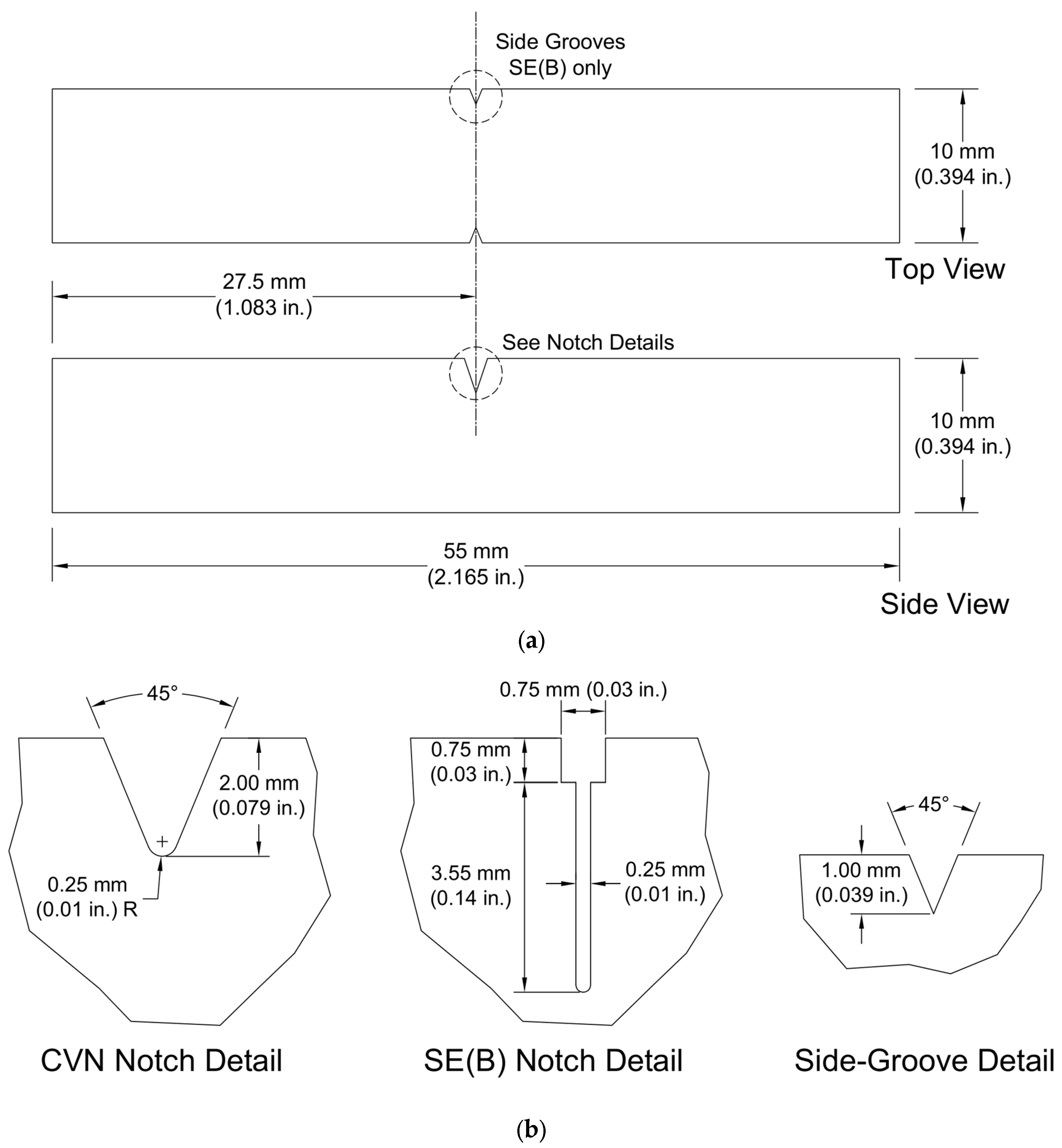
2.1. Charpy V-Notch Impact Testing
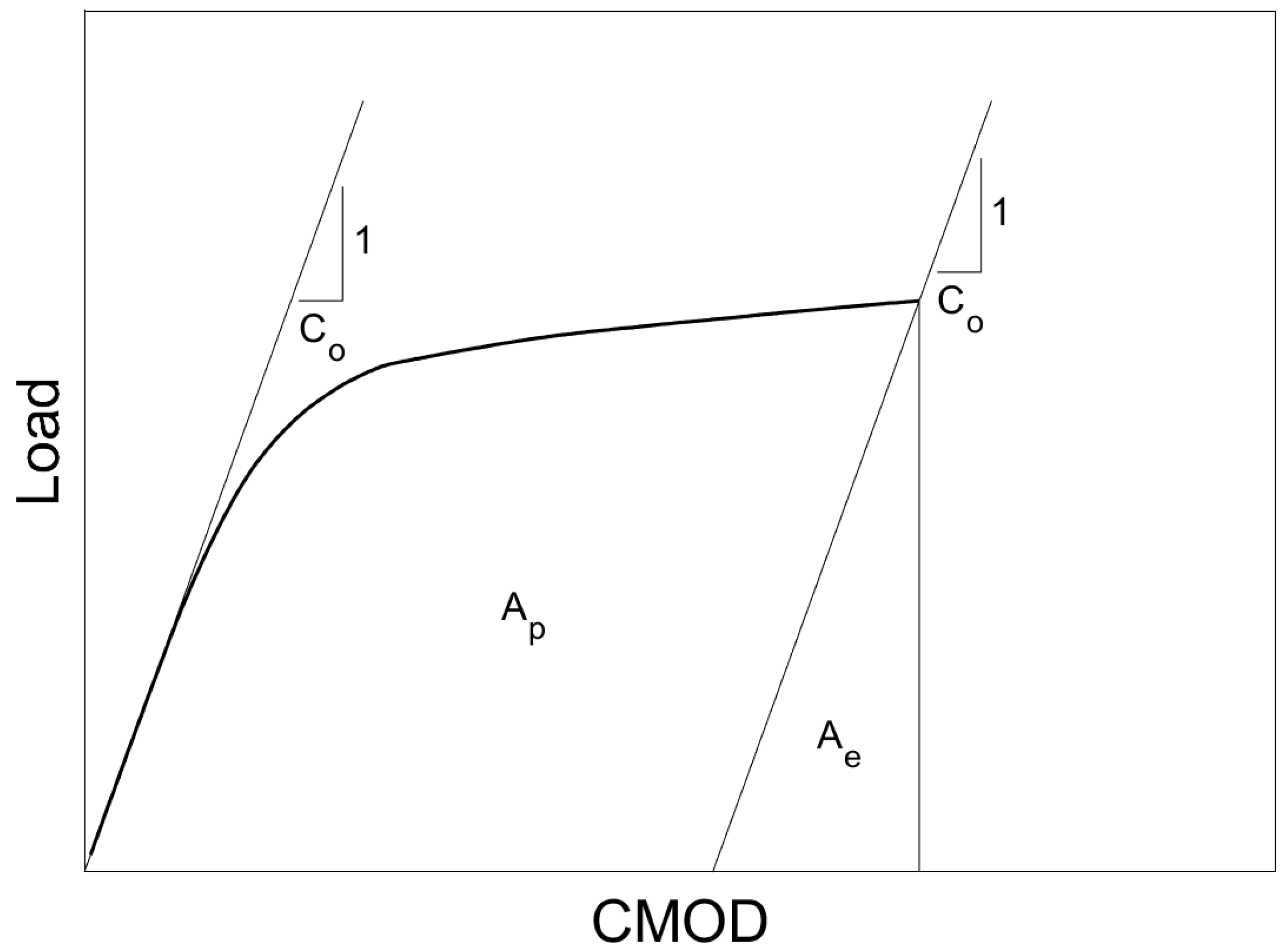
2.2. Fracture Toughness Testing
2.3. Master Curve Analysis
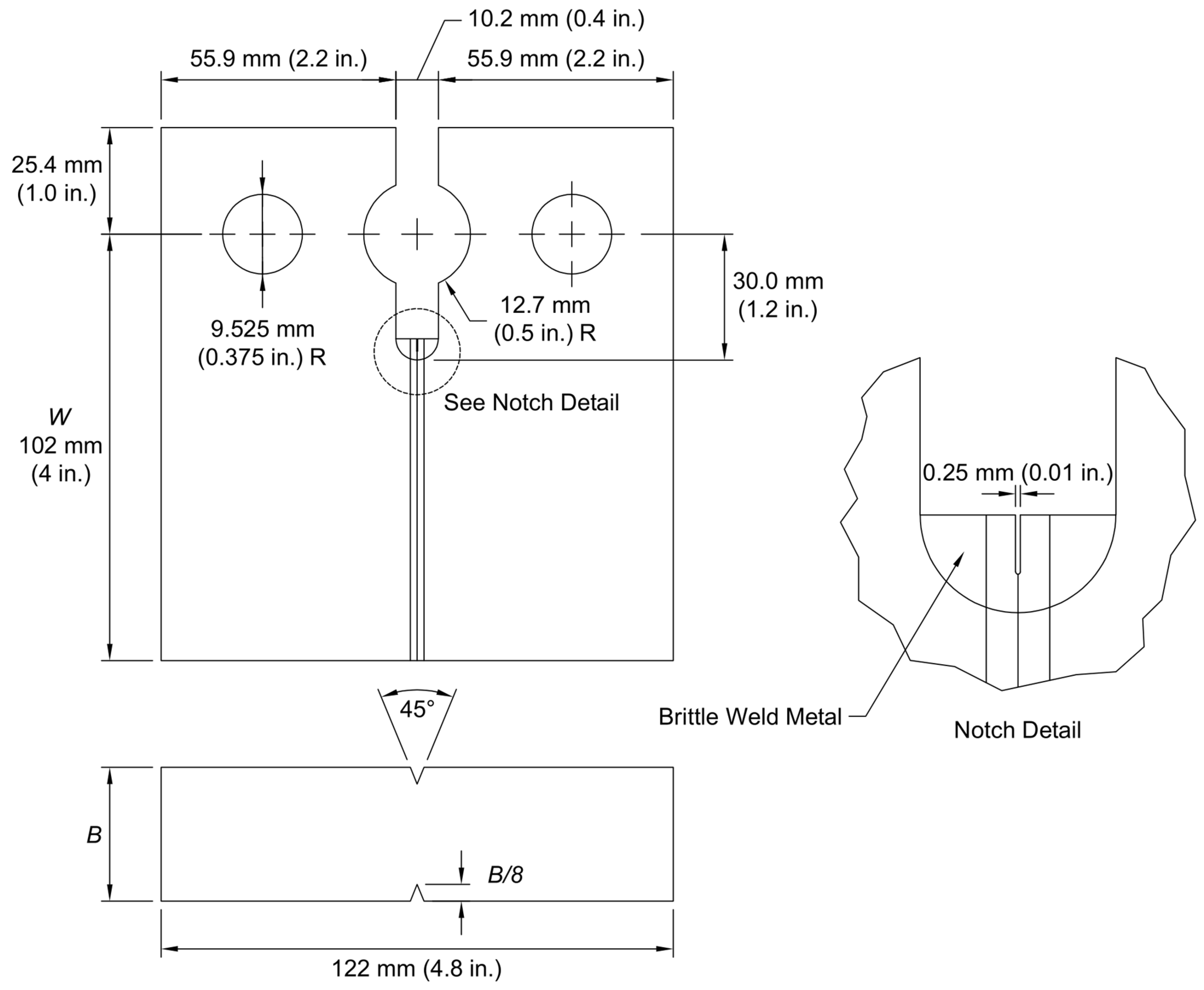
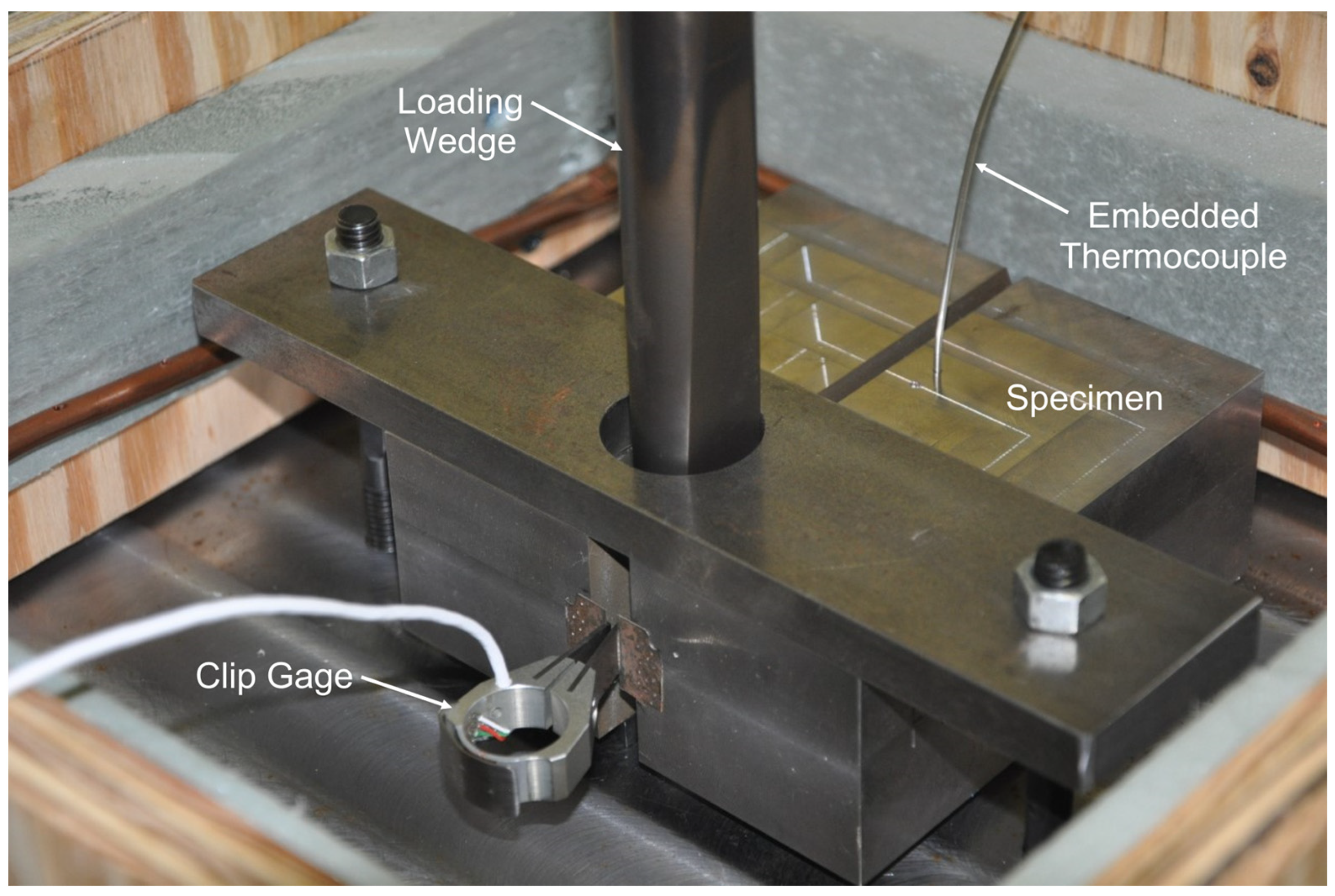
2.4. Crack Arrest Testing
2.5. Impact Energy–Fracture Toughness Correlations
2.6. Stress Intensity Rate Adjustment
3. Results and Discussion
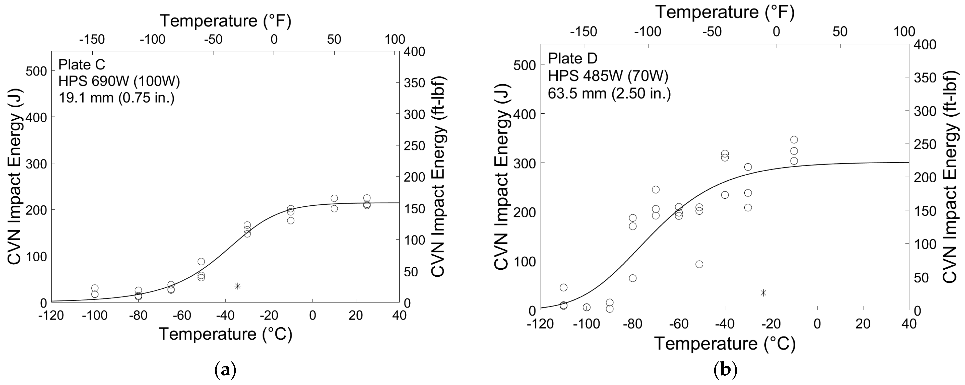
3.1. Charpy V-Notch Results
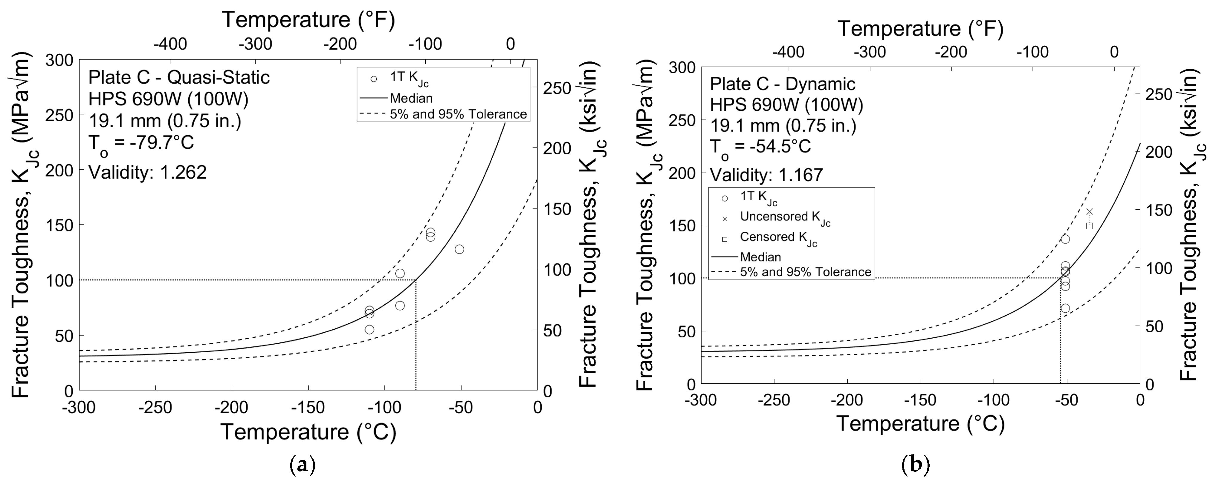
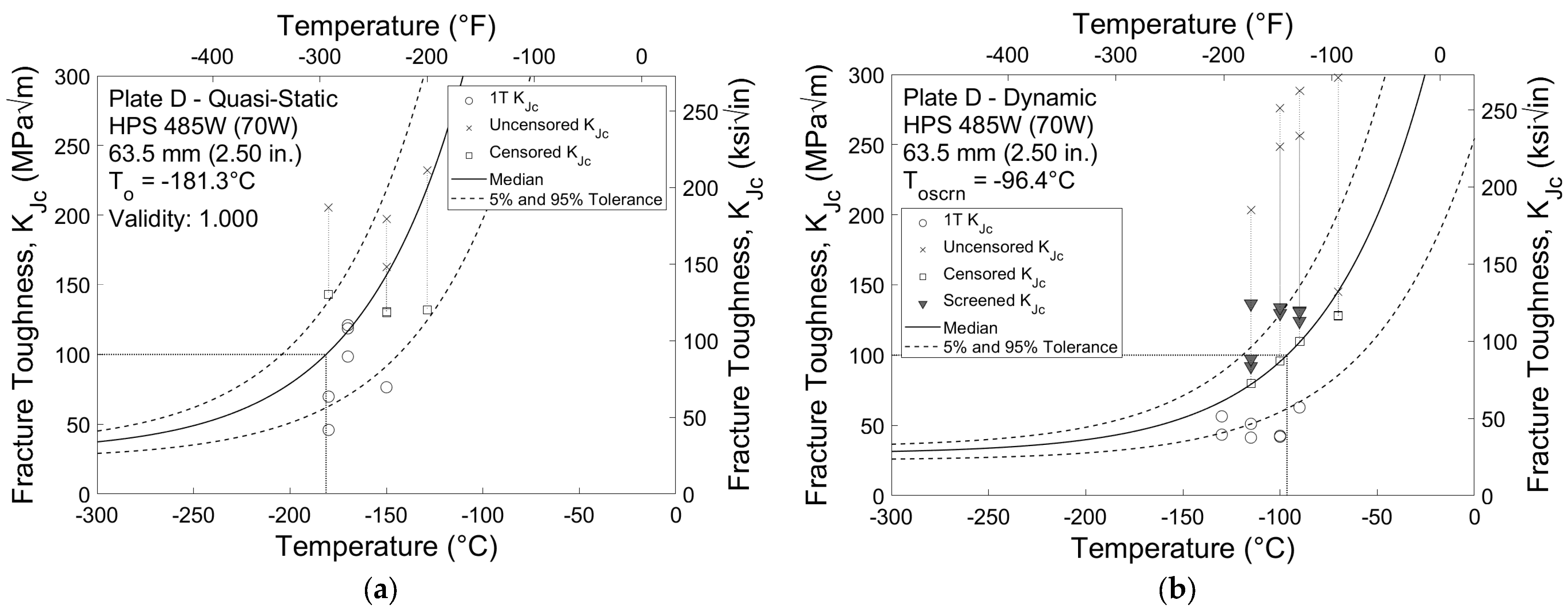
3.2. Fracture Toughness Results
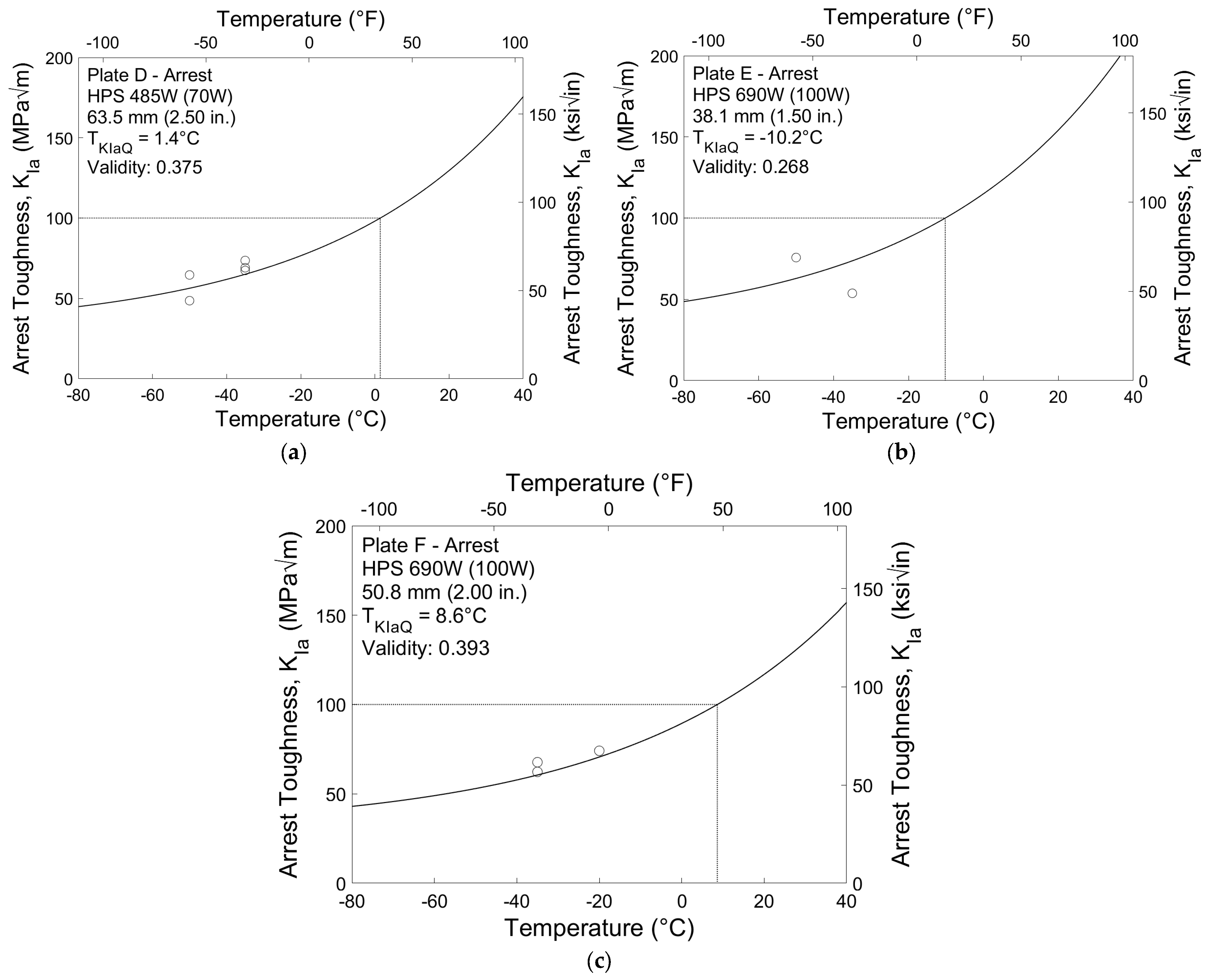
3.3. Crack Arrest Results
3.4. Reference Temperature Rate Adjustment
3.5. Correlation Evaluations
4. Conclusions
Author Contributions
Funding
Institutional Review Board Statement
Informed Consent Statement
Data Availability Statement
Acknowledgments
Conflicts of Interest
Notation
| a | Asymptotic minimum of sigmoid fit; |
| ao | Initial crack size; |
| A | Total area under load-CMOD curve; |
| Ae | Elastic component of area under load-CMOD curve; |
| Ap | Plastic component of area under load-CMOD curve; |
| b | Asymptotic maximum of sigmoid fit; |
| bo | Initial remaining ligament size; |
| B | Specimen thickness; |
| BN | Net specimen thickness; |
| Bo | Initial specimen thickness used in thickness adjustment; |
| Bx | Desired specimen thickness for thickness adjustment; |
| c | Location parameter of sigmoid fit; |
| C(T) | Compact specimen geometry; |
| Co | Compliance, the reciprocal of the initial elastic slope; |
| CV | Average CVN impact energy used in API 579 correlation approach; |
| CVN(T) | Charpy V-notch impact energy at a given temperature, T; |
| CV-LS | Charpy V-notch impact energy at lower shelf behavior; |
| CV-US | Charpy V-notch impact energy at upper shelf behavior; |
| d | Slope parameter of sigmoid fit; |
| E | Modulus of elasticity; |
| Jc | Critical value of J-integral at failure; |
| Je | Elastic component of J-integral calculation; |
| Jp | Plastic component of J-integral calculation; |
| Stress intensity rate; | |
| Kc | Critical fracture toughness; |
| Kdyn | Dynamic fracture toughness; |
| Ke | Elastic fracture toughness; |
| KIa | Crack arrest fracture toughness; |
| KJc | Elastic–plastic equivalent fracture toughness converted from critical J-integral; |
| KJc(0.xx) | Elastic–plastic fracture toughness tolerance limit of xx per cent; |
| KJc(i) | Elastic–plastic fracture toughness of ith specimen; |
| KJclimit | Elastic–plastic fracture toughness limit in master curve analysis; |
| KJc(med) | Median elastic–plastic fracture toughness; |
| KJc(med)eq | Equivalent median toughness used in inhomogeneity screening process |
| KJc(o) | Initial elastic–plastic fracture toughness used in thickness adjustment; |
| KJc(x) | Size adjusted fracture toughness for specimen of thickness BN; |
| Kmin | Absolute minimum fracture toughness equal to 20 MPa√m (18 ksi√in); |
| m | Scale parameter of sigmoid fit; |
| n | Load cycle count in crack arrest testing; |
| r | Number of uncensored data used to determine provisional reference temperature; |
| SA | Percent shear area of CVN fracture surface; |
| SE(B) | Single edge bend specimen geometry; |
| T | Test temperature; |
| T27J | Test temperature corresponding to CVN of 27 J; |
| T28J | Test temperature corresponding to CVN of 28 J; |
| T40J | Test temperature corresponding to CVN of 40 J; |
| Ti | Test temperature of ith specimen; |
| Tk | Temperature adjustment based on CVN scatter in BS 7910; |
| TKIaQ | Provisional arrest reference temperature; |
| To | Reference temperature where median toughness equals 100 MPa√m (91 ksi√in); |
| To,adj | Rate adjusted reference temperature; |
| To,est | Prediction of static reference temperature correlated from CVN data; |
| ToQ | Provisional reference temperature prior to validation; |
| To,scrn | Reference temperature following inhomogeneity screening procedure; |
| To,sta | Quasi-static rate reference temperature; |
| Tshift | Temperature shift rate adjustment in Barsom and Rolfe Two-Stage correlation; |
| W | Specimen width; |
| xT | Specimen thickness designation with x in inches; |
| β | Sample size uncertainty factor used in inhomogeneity screening process; |
| δa | CMOD corresponding to crack arrest; |
| δi | Validity of ith specimen in master curve analysis, valid = 1, invalid = 0; |
| δn,max | Maximum CMOD limit for a given load cycle in crack arrest testing; |
| δo | CMOD corresponding to crack initiation in crack arrest testing; |
| δo,limit | Overall CMOD limit for crack arrest testing; |
| (δp)1 | CMOD offset at the end of the first crack arrest load cycle; |
| (δp)n−1 | CMOD offset at the beginning of the last crack arrest load cycle; |
| ΔTexperimental | Difference between quasi-static and dynamic reference temperature; |
| ΔTtheoretical | Theoretical rate-dependent shift applied to reference temperature; |
| Γ | Material fitting coefficient used in Wallin rate adjustment; |
| σys | 0.2% offset yield strength; |
| ν | Poisson’s ratio. |
References
- Barsom, J.M.; Rolfe, S.T. Correlations between KIc and Charpy V-Notch Test Results in the Transition-Temperature Range; ASTM STP 32067S; ASTM International: West Conshohocken, PA, USA, 1970; pp. 281–302. [Google Scholar]
- Corten, H.T.; Sailors, R.H. Relationship between Material Fracture Toughness Using Fracture Mechanics and Transition Temperature Tests; ASTM STP 38825S; ASTM International: West Conshohocken, PA, USA, 1971; pp. 164–191. [Google Scholar]
- Barsom, J.M. Development of the AASHTO fracture-toughness requirements for bridge steels. Eng. Fracture Mech. 1975, 7, 605–618. [Google Scholar] [CrossRef]
- Marandet, B.; Sanz, G. Evaluation of the Toughness of Thick Medium Strength Steels by LEFM and Correlations between KIc and CVN; ASTM STP 631; ASTM International: West Conshohocken, PA, USA, 1977; pp. 72–95. [Google Scholar]
- BS 7910:2013; Guide to Methods for Assessing the Acceptability of Flaws in Metallic Structures. British Standards Institution: London, UK, 2013.
- API 579/ASME FFS-1 2021; Fitness-For-Service. API Publishing Services: Washington, DC, USA, 2021.
- American Association of State Highway and Transportation Officials. AASHTO LRFD Bridge Design Specifications, 8th ed.; AASHTO: Washington, DC, USA, 2020. [Google Scholar]
- Wallin, K. The scatter in KIc Results. Eng. Fract. Mech. 1984, 19, 1085–1093. [Google Scholar] [CrossRef]
- Wallin, K. Effect of strain rate on the fracture toughness reference temperature to for ferritic steels. In Recent Advances in Fracture, Proceedings of a Symposium Held at the ANNUAL Meeting of The Minerals, Metals and Materials Society, Orlando, FL, USA, 10–13 February 1997; Mahidhara, R.K., Geltmacher, A., Matic, P., Sadananda, K., Eds.; The Minerals, Metals, and Materials Society: Warrendale, PA, USA, 1997; pp. 171–182. [Google Scholar]
- E1921-21; Standard Test Method for Determination of Reference Temperature, to, for Ferritic Steels in the Transition Range. ASTM International: West Conshohocken, PA, USA, 2021.
- E1820-20; Standard Test Method for Fracture Toughness. ASTM International: West Conshohocken, PA, USA, 2020.
- Gao, X.; Dodds, R.H. Loading rate effects on parameters of the Weibull stress model for ferritic steels. Eng. Fract. Mech. 2005, 72, 2416–2425. [Google Scholar] [CrossRef]
- Gao, X.; Joyce, J.A.; Roe, C. An Investigation of the Loading Rate Dependence of the Weibull Stress Parameters. Eng. Fract. Mech. 2008, 75, 1451–1467. [Google Scholar] [CrossRef]
- Collins, W. Fracture Behavior Characterization of Conventional and High Performance Steel for Bridge Applications. Ph.D. Dissertation, Virginia Polytechnic Institute and State University, Blacksburg, VA, USA, 13 November 2014. [Google Scholar]
- Collins, W.; Sherman, R.; Connor, R. Fracture Characterization of High Performance Steel; Final Report Part 1 for TPF-5(238); Purdue University: West Lafayette, IN, USA, 2015. [Google Scholar]
- Sherman, R.; Collins, W.; Connor, R. Material characterization of high-toughness steel. Structures 2019, 20, 33–41. [Google Scholar] [CrossRef]
- Collins, W.; Sherman, R.; Leon, R.; Connor, R. Fracture Toughness Characterization of High-Performance Steel for Bridge Girder Applications. J. Mater. Civ. Eng. 2019, 31, 04019027. [Google Scholar] [CrossRef]
- Hamby, G.; Clinton, R.; Lwin, M. High Performance Steel Designers’ Guide, 2nd ed.; U.S. Department of Transportation, Federal Highway Administration: Washington, DC, USA, 2002.
- Wilson, A.D. Development of an improved HPS-100W steel for bridge applications. In International Symposium on Microalloyed Steels; ASM International: Materials Park, OH, USA, 2002. [Google Scholar]
- Wright, W.J. Fracture Initiation and Resistance of I-Girders Fabricated from High Performance Steels. Doctoral Dissertation, Lehigh University, Bethlehem, PA, USA, 2003. [Google Scholar]
- Kayser, C.; Swanson, J.; Linzell, D. Characterization of material properties of HPS-485W (70W) TMCP for bridge girder applications. J. Bridge Eng. 2006, 11, 99–108. [Google Scholar] [CrossRef]
- Sherman, R.; Collins, W.; Connor, R. Large-Scale Axial Fracture Experiments of High-Toughness Steel. J. Bridge Eng. 2020, 25, 04020070. [Google Scholar] [CrossRef]
- Sherman, R.; Collins, W.; Connor, R. Large-Scale Flexure Fracture Experiments of High-Toughness Steel. J. Bridge Eng. 2019, 24, 04019062. [Google Scholar] [CrossRef]
- A709-13; Standard Specification for Structural Steel for Bridges. ASTM International: West Conshohocken, PA, USA, 2013.
- A673-17; Standard Specification for Sampling Procedure for Impact Testing of Structural Steel. ASTM International: West Conshohocken, PA, USA, 2017.
- Yount, T.; Sorensen, T.; Collins, W.; Maguire, M. Investigating the Mechanical Properties and Fracture Behavior of Welded-Wire Reinforcement. J. Mater. Civ. Eng. 2021, 33, 04021023. [Google Scholar] [CrossRef]
- E1921-13; Standard Test Method for Determination of Reference Temperature, to, for Ferritic Steels in the Transition Range. ASTM International: West Conshohocken, PA, USA, 2013.
- E647-13; Standard Test Method for Measurement of Fatigue Crack Growth Rates. ASTM International: West Conshohocken, PA, USA, 2013.
- E1221-12; Standard Test Method For Determining Plane-Strain Crack-Arrest Fracture Toughness, KIa, of Ferritic Steels. ASTM International: West Conshohocken, PA, USA, 2012.
- Collins, W.; Sherman, R.; Leon, R.; Connor, R. State-of-the-art fracture characterization. II: Correlations between Charpy V-notch and the master curve reference temperature. J. Bridge Eng. 2016, 21, 04016098. [Google Scholar] [CrossRef]
- A709-21; Standard Specification for Structural Steel for Bridges. ASTM International: West Conshohocken, PA, USA, 2021.


| Plate | Grade MPa (ksi) | Thickness mm (in) | CVN Impact | Charpy-Sized SE(B) | Crack Arrest | |
|---|---|---|---|---|---|---|
| Static | Dynamic | |||||
| A | 485 (70) | 25.4 (1.00) | 24 (24) | 9 (8) | 11 (10) | - |
| C | 690 (100) | 19.1 (0.75) | 24 (24) | 8 (8) | 8 (8) | - |
| D | 485 (70) | 63.5 (2.50) | 24 (23) | 13 (10) | 17 (17) | 10 (5) |
| E | 690 (100) | 38.1 (1.50) | 24 (23) | 15 (12) | 13 (13) | 5 (2) |
| F | 690 (100) | 50.8 (2.00) | 24 (24) | 15 (11) | 12 (12) | 3 (3) |
| H | 485 (70) | 31.8 (1.25) | 24 (24) | 10 (10) | 8 (8) | - |
| I | 485 (70) | 31.8 (1.25) | 24 (24) | 9 (8) | 8 (8) | - |
| J | 485 (70) | 38.1 (1.50) | 24 (23) | 8 (8) | 10 (10) | - |
| Temperature Range, T–To °C (°F) | Weighting Factor |
|---|---|
| +50 to −14 (+90 to −25) | 1/6 |
| −15 to −35 (−27 to −63) | 1/7 |
| −36 to −50 (−65 to −90) | 1/8 |
| Grade MPa (ksi) | Plate | T27J °C (°F) | T40J °C (°F) | To,est, °C (°F) | ||
|---|---|---|---|---|---|---|
| B and R | BS 7910 | API 579 | ||||
| 690 (100) | C | −71 (−96) | −63 (−81) | −62 (−80) | −63 (−81) | −59 (−74) |
| E | −81 (−113) | −73 (−100) | −73 (−100) | −73 (−99) | −69 (−93) | |
| F | −88 (−127) | −78 (−108) | −77 (−106) | −79 (−110) | −76 (−105) | |
| 485 (70) | A | −119 (−183) | −110 (−166) | −143 (−225) | −111 (−167) | −131 (−204) |
| D | −103 (−153) | −98 (−144) | −105 (−157) | −96 (−141) | −115 (−175) | |
| H | −89 (−129) | −86 (−124) | −114 (−174) | −84 (−119) | −102 (−151) | |
| I | −91 (−132) | −87 (−124) | −124 (−191) | −85 (−121) | −105 (−156) | |
| J | −104 (−156) | −97 (−142) | −125 (−194) | −97 (−142) | −116 (−177) | |
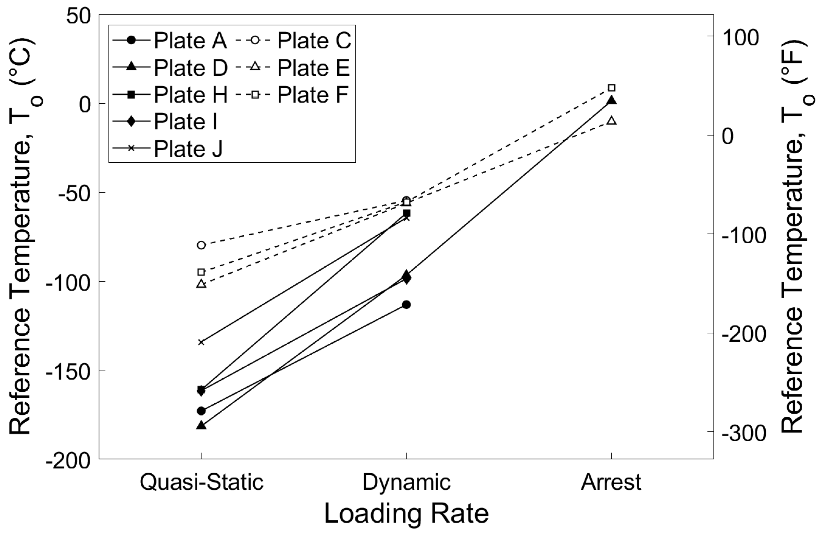
| Grade MPa (ksi) | Plate | Stress Intensity Rate | Validity | Reference Temperature °C (°F) |
|---|---|---|---|---|
| 690 (100) | C | Quasi-Static | 1.262 | −80 (−111) |
| Dynamic | 1.167 | −55 (−66) | ||
| E | Quasi-Static | 1.476 | −102 (−151) | |
| Dynamic | 1.833 | −56 (−69) | ||
| F | Quasi-Static | 1.214 | −95 (−139) | |
| Dynamic | 1.619 | −55 (−68) | ||
| 485 (70) | A | Quasi-Static | 1.000 | −173 (−279) |
| Dynamic | 1.500 | −113 (−172) | ||
| D | Quasi-Static | 1.000 | −181 (−294) | |
| Dynamic | - | −96 (−142) | ||
| H | Quasi-Static | 1.000 | −161 (−258) | |
| Dynamic | - | −62 (−79) | ||
| I | Quasi-Static | - | −161 (−259) | |
| Dynamic | - | −98 (−145) | ||
| J | Quasi-Static | 1.095 | −134 (−209) | |
| Dynamic | 1.196 | −64 (−84) |
| Grade MPa (ksi) | Plate | Mean Stress Intensity Rate, MPa√m/s (ksi√in/s) | ΔTtheoretical °C (°F) | Tshift °C (°F) | ΔTexperimental °C (°F) |
|---|---|---|---|---|---|
| 690 (100) | C | 2720 (2470) | 24 (43) | 36 (65) | 25 (45) |
| E | 3270 (2980) | 27 (49) | 36 (65) | 46 (82) | |
| F | 3230 (2940) | 26 (47) | 36 (65) | 40 (71) | |
| 485 (70) | A | 3020 (2750) | 43 (78) | 61 (110) | 60 (108) |
| D | 2820 (2570) | 42 (75) | 61 (110) | 85 (153) | |
| H | 3540 (3220) | 45 (81) | 61 (110) | 99 (179) | |
| I | 3350 (3050) | 44 (80) | 61 (110) | 63 (113) | |
| J | 3650 (3320) | 44 (79) | 61 (110) | 70 (126) |
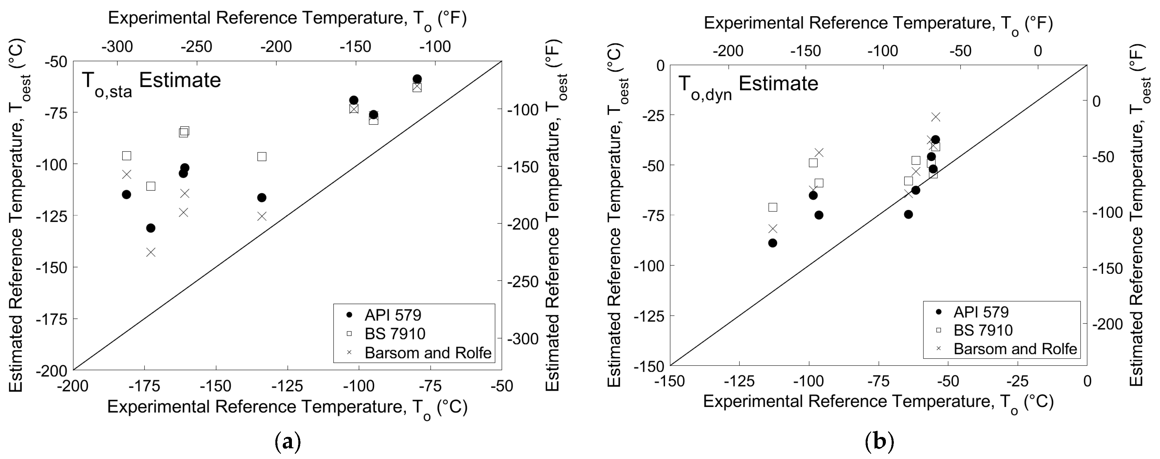
| Grade MPa (ksi) | Plate | Stress Intensity Rate | To °C (°F) | To,est °C (°F) | ||
|---|---|---|---|---|---|---|
| B and R | BS 7910 | API 579 | ||||
| 690 (100) | C | Quasi-Static | −80 (−111) | −62 (−80) | −63 (−81) | −59 (−74) |
| Dynamic | −55 (−66) | −26 (−15) | −41 (−42) | −37 (−35) | ||
| E | Quasi-Static | −102 (−151) | −73 (−100) | −73 (−99) | −69 (−93) | |
| Dynamic | −56 (−69) | −37 (−35) | −49 (−57) | −46 (−50) | ||
| F | Quasi-Static | −95 (−139) | −77 (−106) | −79 (−110) | −76 (−105) | |
| Dynamic | −55 (−68) | −40 (−41) | −54 (−66) | −52 (−62) | ||
| 485 (70) | A | Quasi-Static | −173 (−279) | −143 (−225) | −111 (−167) | −131 (−204) |
| Dynamic | −113 (−172) | −82 (−115) | −71 (−96) | −89 (−128) | ||
| D | Quasi-Static | −181 (−294) | −105 (−157) | −96 (−141) | −115 (−175) | |
| Dynamic | −96 (−142) | −44 (−47) | −59 (−74) | −75 (−103) | ||
| H | Quasi-Static | −161 (−258) | −114 (−174) | −84 (−119) | −102 (−151) | |
| Dynamic | −62 (−79) | −53 (−64) | −48 (−54) | −63 (−81) | ||
| I | Quasi-Static | −161 (−259) | −124 (−191) | −85 (−121) | −105 (−156) | |
| Dynamic | −98 (−145) | −63 (−81) | −49 (−56) | −65 (−85) | ||
| J | Quasi-Static | −134 (−209) | −125 (−194) | −97 (−142) | −116 (−177) | |
| Dynamic | −64 (−84) | −64 (−84) | −58 (−72) | −75 (−102) | ||
Disclaimer/Publisher’s Note: The statements, opinions and data contained in all publications are solely those of the individual author(s) and contributor(s) and not of MDPI and/or the editor(s). MDPI and/or the editor(s) disclaim responsibility for any injury to people or property resulting from any ideas, methods, instructions or products referred to in the content. |
© 2023 by the authors. Licensee MDPI, Basel, Switzerland. This article is an open access article distributed under the terms and conditions of the Creative Commons Attribution (CC BY) license (https://creativecommons.org/licenses/by/4.0/).
Share and Cite
Collins, W.N.; Yount, T.D.; Sherman, R.J.; Leon, R.T.; Connor, R.J. Dynamic Fracture and Crack Arrest Toughness Evaluation of High-Performance Steel Used in Highway Bridges. Materials 2023, 16, 3402. https://doi.org/10.3390/ma16093402
Collins WN, Yount TD, Sherman RJ, Leon RT, Connor RJ. Dynamic Fracture and Crack Arrest Toughness Evaluation of High-Performance Steel Used in Highway Bridges. Materials. 2023; 16(9):3402. https://doi.org/10.3390/ma16093402
Chicago/Turabian StyleCollins, William N., Tristan D. Yount, Ryan J. Sherman, Roberto T. Leon, and Robert J. Connor. 2023. "Dynamic Fracture and Crack Arrest Toughness Evaluation of High-Performance Steel Used in Highway Bridges" Materials 16, no. 9: 3402. https://doi.org/10.3390/ma16093402