

Computational Complexity and Its Influence on Predictive Capabilities of Machine Learning Models for Concrete Mix Design


Abstract
:1. Introduction
2. Concrete Mix Design and Machine Learning
2.1. Prediction of Concrete Technical Properties in Concrete Mix Design
2.2. Machine Learning in Prediction of Concrete Technical Properties
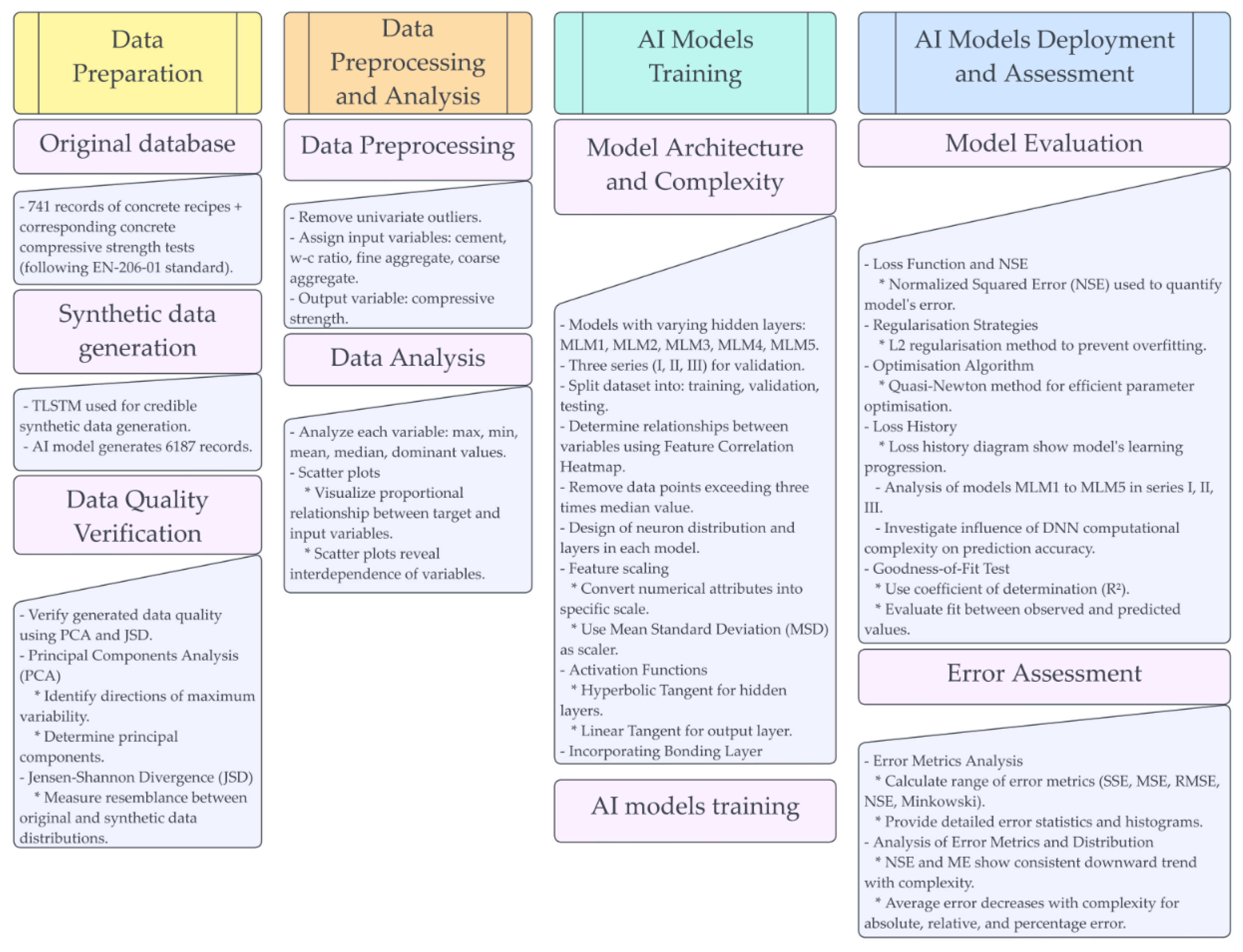
3. Materials and Methods
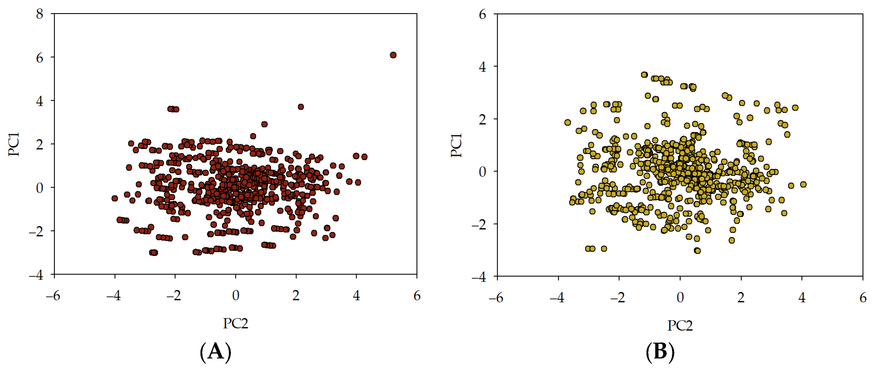
3.1. Essentials
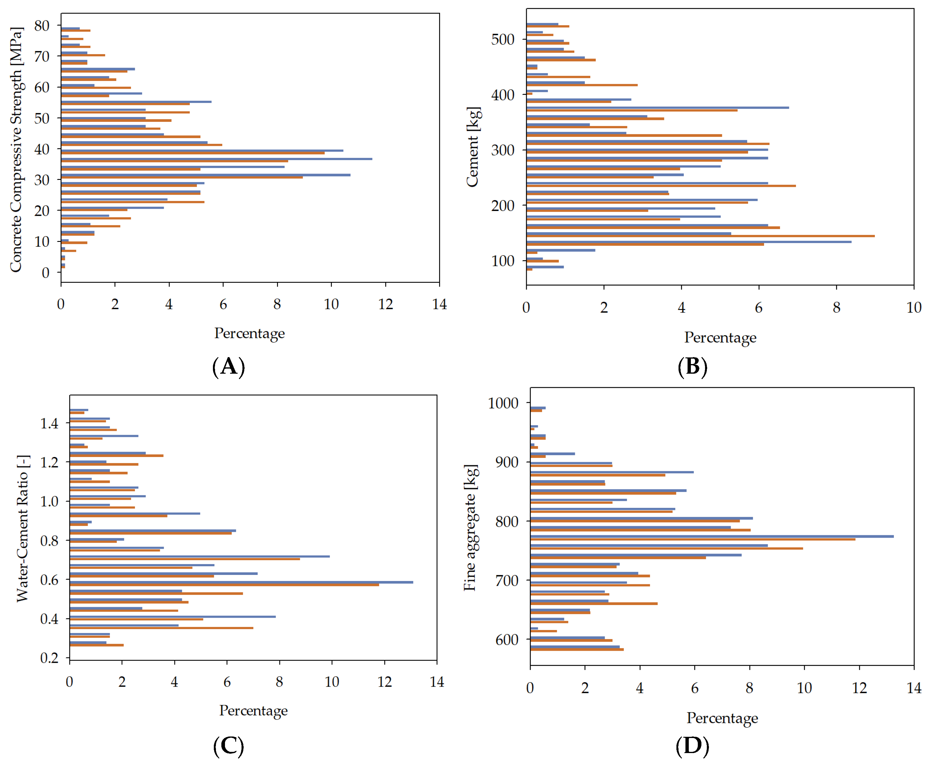
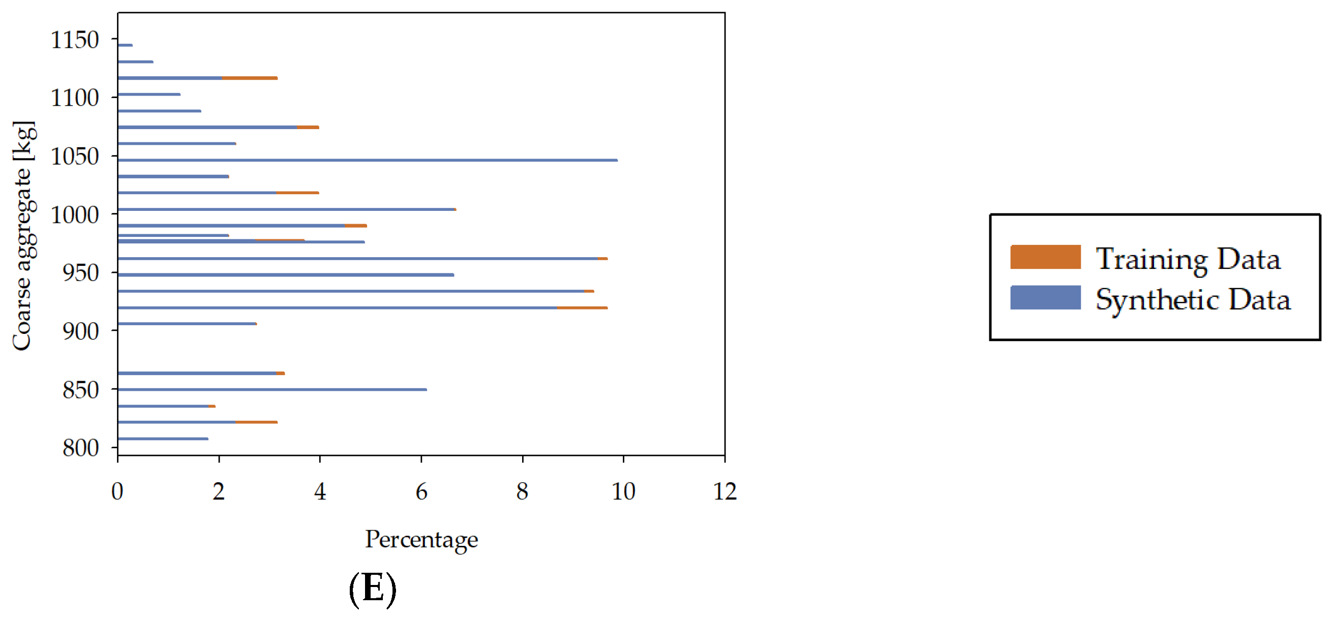
3.2. Data Processing
3.3. Training, Testing, and Model Selection
3.4. Results and Discussion
4. Summary and Conclusions
Funding
Institutional Review Board Statement
Informed Consent Statement
Data Availability Statement
Conflicts of Interest
References
- Suchorzewski, J.; Prieto, M.; Mueller, U. An Experimental Study of Self-Sensing Concrete Enhanced with Multi-Wall Carbon Nanotubes in Wedge Splitting Test and DIC. Constr. Build. Mater. 2020, 262, 120871. [Google Scholar] [CrossRef]
- Nowek, A.; Kaszubski, P.; Abdelgader, H.S.; Górski, J. Effect of Admixtures on Fresh Grout and Two-Stage (Pre-Placed Aggregate) Concrete. Struct. Concr. 2007, 8, 17–23. [Google Scholar] [CrossRef]
- Kujawa, W.; Olewnik-Kruszkowska, E.; Nowaczyk, J. Concrete Strengthening by Introducing Polymer-Based Additives into the Cement Matrix-a Mini Review. Materials 2021, 14, 6071. [Google Scholar] [CrossRef]
- Suchorzewski, J.; Chitvoranund, N.; Srivastava, S.; Prieto, M.; Malaga, K. Recycling Potential of Cellular Lightweight Concrete Insulation as Supplementary Cementitious Material. In Proceedings of the RILEM Bookseries; Springer: Berlin/Heidelberg, Germany, 2023; Volume 44, pp. 133–141. [Google Scholar]
- Liu, G.; Cheng, W.; Chen, L.; Pan, G.; Liu, Z. Rheological Properties of Fresh Concrete and Its Application on Shotcrete. Constr. Build. Mater. 2020, 243, 118180. [Google Scholar] [CrossRef]
- McNamee, R.; Sjöström, J.; Boström, L. Reduction of Fire Spalling of Concrete with Small Doses of Polypropylene Fibres. Fire Mater. 2021, 45, 943–951. [Google Scholar] [CrossRef]
- Cos-Gayón López, F.; Benlloch Marco, J.; Calvet Rodríguez, V. Influence of High Temperatures on the Bond between Carbon Fibre-Reinforced Polymer Bars and Concrete. Constr. Build. Mater. 2021, 309, 124967. [Google Scholar] [CrossRef]
- Gupta, S.; Kua, H.W.; Pang, S.D. Effect of Biochar on Mechanical and Permeability Properties of Concrete Exposed to Elevated Temperature. Constr. Build. Mater. 2020, 234, 117338. [Google Scholar] [CrossRef]
- Marchon, D.; Flatt, R.J. Mechanisms of Cement Hydration. Sci. Technol. Concr. Admix. 2016, 41, 129–145. [Google Scholar] [CrossRef]
- Liu, Y.; Kumar, D.; Lim, K.H.; Lai, Y.L.; Hu, Z.; Ambikakumari Sanalkumar, K.U.; Yang, E.H. Efficient Utilization of Municipal Solid Waste Incinerator Bottom Ash for Autoclaved Aerated Concrete Formulation. J. Build. Eng. 2023, 71, 106463. [Google Scholar] [CrossRef]
- Kocaba, V.; Gallucci, E.; Scrivener, K.L. Methods for Determination of Degree of Reaction of Slag in Blended Cement Pastes. Cem. Concr. Res. 2012, 42, 511–525. [Google Scholar] [CrossRef]
- Boinski, T.; Chojnowski, A. Towards Facts Extraction from Text in Polish Language. In Proceedings of the 2017 IEEE International Conference on INnovations in Intelligent SysTems and Applications, INISTA 2017, Gdynia, Poland, 3–5 July 2017; IEEE: Piscataway, NJ, USA, 2017; pp. 13–17. [Google Scholar]
- Pawlicki, M.; Marchewka, A.; Choraś, M.; Kozik, R. Gated Recurrent Units for Intrusion Detection. In Proceedings of the Advances in Intelligent Systems and Computing; Springer: Cham, Switzerland, 2020; Volume 1062, pp. 142–148. [Google Scholar]
- Renigier-Biłozor, M.; Janowski, A.; d’Amato, M. Automated Valuation Model Based on Fuzzy and Rough Set Theory for Real Estate Market with Insufficient Source Data. Land Use Policy 2019, 87, 104021. [Google Scholar] [CrossRef]
- Renigier-Biłozor, M.; Chmielewska, A.; Walacik, M.; Janowski, A.; Lepkova, N. Genetic Algorithm Application for Real Estate Market Analysis in the Uncertainty Conditions. J. Hous. Built Environ. 2021, 36, 1629–1670. [Google Scholar] [CrossRef]
- Renigier-Biłozor, M.; Janowski, A.; Walacik, M.; Chmielewska, A. Modern Challenges of Property Market Analysis-Homogeneous Areas Determination. Land Use Policy 2022, 119, 106209. [Google Scholar] [CrossRef]
- Chmielewska, A.; Renigier-Biłozor, M.; Janowski, A. Representative Residential Property Model—Soft Computing Solution. Int. J. Environ. Res. Public Health 2022, 19, 15114. [Google Scholar] [CrossRef]
- De Prado, R.P.; García-Galán, S.; Muñoz-Expósito, J.E.; Marchewka, A. Acceleration of Genome Sequencing with Intelligent Cloud Brokers. In Proceedings of the Advances in Intelligent Systems and Computing; Springer: Cham, Switzerland, 2018; Volume 681, pp. 133–140. [Google Scholar]
- Van Engelen, J.E.; Hoos, H.H. A Survey on Semi-Supervised Learning. Mach. Learn. 2020, 109, 373–440. [Google Scholar]
- Sutton, R.S.; Barto, A.G. Reinforcement Learning: An Introduction; MIT Press: Cambridge, MA, USA, 2018; ISBN 0262352702. [Google Scholar]
- Li, Y. Deep Reinforcement Learning: An Overview. arXiv 2017, arXiv:1701.07274. [Google Scholar]
- Ambroziak, A.; Ziolkowski, P. Concrete Compressive Strength under Changing Environmental Conditions during Placement Processes. Materials 2020, 13, 4577. [Google Scholar] [CrossRef] [PubMed]
- Tam, C.T.; Babu, D.S.; Li, W. EN 206 Conformity Testing for Concrete Strength in Compression. Procedia Eng. 2017, 171, 227–237. [Google Scholar] [CrossRef]
- EN 1992-1-1: 2004; Eurocode 2: Design of Concrete Structures. British Standards Institution: London, UK, 2004.
- DIN EN 206-1:2001-07; Beton–Teil 1: Festlegung, Eigenschaften, Herstellung Und Konformität; Deutsche Fassung EN 206-1:2000. German Institute for Standardisation: Berlin, Germany, 2001.
- Abdelgader, H.S.; El-Baden, A.S.; Shilstone, J.M. Bolomeya Model for Normal Concrete Mix Design. J. Concr. Plant Int. 2012, 2, 68–74. [Google Scholar]
- Zhang, C.; Nerella, V.N.; Krishna, A.; Wang, S.; Zhang, Y.; Mechtcherine, V.; Banthia, N. Mix Design Concepts for 3D Printable Concrete: A Review. Cem. Concr. Compos. 2021, 122, 104155. [Google Scholar] [CrossRef]
- Li, N.; Shi, C.; Zhang, Z.; Wang, H.; Liu, Y. A Review on Mixture Design Methods for Geopolymer Concrete. Compos. Part B Eng. 2019, 178, 107490. [Google Scholar] [CrossRef]
- Liu, Q.F.; Iqbal, M.F.; Yang, J.; Lu, X.Y.; Zhang, P.; Rauf, M. Prediction of Chloride Diffusivity in Concrete Using Artificial Neural Network: Modelling and Performance Evaluation. Constr. Build. Mater. 2021, 268, 121082. [Google Scholar] [CrossRef]
- Iqbal, M.F.; Liu, Q.F.; Azim, I.; Zhu, X.; Yang, J.; Javed, M.F.; Rauf, M. Prediction of Mechanical Properties of Green Concrete Incorporating Waste Foundry Sand Based on Gene Expression Programming. J. Hazard. Mater. 2020, 384, 121322. [Google Scholar] [CrossRef] [PubMed]
- Yeh, I.C. Modeling of Strength of High-Performance Concrete Using Artificial Neural Networks. Cem. Concr. Res. 1998, 28, 1797–1808. [Google Scholar] [CrossRef]
- Lee, S.C. Prediction of Concrete Strength Using Artificial Neural Networks. Eng. Struct. 2003, 25, 849–857. [Google Scholar] [CrossRef]
- Hola, J.; Schabowicz, K. Application of Artificial Neural Networks to Determine Concrete Compressive Strength Based on Non-Destructive Tests. J. Civ. Eng. Manag. 2005, 11, 23–32. [Google Scholar] [CrossRef]
- Hola, J.; Schabowicz, K. New Technique of Nondestructive Assessment of Concrete Strength Using Artificial Intelligence. NDT E Int. 2005, 38, 251–259. [Google Scholar] [CrossRef]
- Gupta, R.; Kewalramani, M.A.; Goel, A. Prediction of Concrete Strength Using Neural-Expert System. J. Mater. Civ. Eng. 2006, 18, 462–466. [Google Scholar] [CrossRef]
- Bui, D.K.; Nguyen, T.; Chou, J.S.; Nguyen-Xuan, H.; Ngo, T.D. A Modified Firefly Algorithm-Artificial Neural Network Expert System for Predicting Compressive and Tensile Strength of High-Performance Concrete. Constr. Build. Mater. 2018, 180, 320–333. [Google Scholar] [CrossRef]
- Deng, F.; He, Y.; Zhou, S.; Yu, Y.; Cheng, H.; Wu, X. Compressive Strength Prediction of Recycled Concrete Based on Deep Learning. Constr. Build. Mater. 2018, 175, 562–569. [Google Scholar] [CrossRef]
- Naderpour, H.; Rafiean, A.H.; Fakharian, P. Compressive Strength Prediction of Environmentally Friendly Concrete Using Artificial Neural Networks. J. Build. Eng. 2018, 16, 213–219. [Google Scholar] [CrossRef]
- Ziolkowski, P.; Niedostatkiewicz, M. Machine Learning Techniques in Concrete Mix Design. Materials 2019, 12, 1256. [Google Scholar] [CrossRef] [PubMed]
- McCormac, J.C.; Brown, R.H. Design of Reinforced Concrete; John Wiley & Sons: Hoboken, NJ, USA, 2015; ISBN 1118879104. [Google Scholar]
- Nunez, I.; Marani, A.; Nehdi, M.L. Mixture Optimization of Recycled Aggregate Concrete Using Hybrid Machine Learning Model. Materials 2020, 13, 4331. [Google Scholar] [CrossRef] [PubMed]
- Marani, A.; Jamali, A.; Nehdi, M.L. Predicting Ultra-High-Performance Concrete Compressive Strength Using Tabular Generative Adversarial Networks. Materials 2020, 13, 4757. [Google Scholar] [CrossRef] [PubMed]
- Ziolkowski, P.; Niedostatkiewicz, M.; Kang, S.B. Model-Based Adaptive Machine Learning Approach in Concrete Mix Design. Materials 2021, 14, 1661. [Google Scholar] [CrossRef]
- Adil, M.; Ullah, R.; Noor, S.; Gohar, N. Effect of Number of Neurons and Layers in an Artificial Neural Network for Generalized Concrete Mix Design. Neural Comput. Appl. 2022, 34, 8355–8363. [Google Scholar] [CrossRef]
- Feng, W.; Wang, Y.; Sun, J.; Tang, Y.; Wu, D.; Jiang, Z.; Wang, J.; Wang, X. Prediction of Thermo-Mechanical Properties of Rubber-Modified Recycled Aggregate Concrete. Constr. Build. Mater. 2022, 318, 125970. [Google Scholar] [CrossRef]
- Tavares, C.; Wang, X.; Saha, S.; Grasley, Z. Machine Learning-Based Mix Design Tools to Minimize Carbon Footprint and Cost of UHPC. Part 1: Efficient Data Collection and Modeling. Clean. Mater. 2022, 4, 100082. [Google Scholar] [CrossRef]
- Tavares, C.; Grasley, Z. Machine Learning-Based Mix Design Tools to Minimize Carbon Footprint and Cost of UHPC. Part 2: Cost and Eco-Efficiency Density Diagrams. Clean. Mater. 2022, 4, 100094. [Google Scholar] [CrossRef]
- Endzhievskaya, I.G.; Endzhievskiy, A.S.; Galkin, M.A.; Molokeev, M.S. Machine Learning Methods in Assessing the Effect of Mixture Composition on the Physical and Mechanical Characteristics of Road Concrete. J. Build. Eng. 2023, 76, 107248. [Google Scholar] [CrossRef]
- Taffese, W.Z.; Espinosa-Leal, L. Multitarget Regression Models for Predicting Compressive Strength and Chloride Resistance of Concrete. J. Build. Eng. 2023, 72, 106523. [Google Scholar] [CrossRef]
- Gulli, A.; Pal, S. Deep Learning with Keras: Beginners Guide to Deep Learning with Keras; Packt Publishing Ltd.: Birmingham, UK, 2017; ISBN 9781787128422. [Google Scholar]
- Cichy, R.M.; Kaiser, D. Deep Neural Networks as Scientific Models. Trends Cogn. Sci. 2019, 23, 305–317. [Google Scholar] [CrossRef]
- Saxena, A. An Introduction to Convolutional Neural Networks. Int. J. Res. Appl. Sci. Eng. Technol. 2022, 10, 943–947. [Google Scholar] [CrossRef]
- Li, Z.; Liu, F.; Yang, W.; Peng, S.; Zhou, J. A Survey of Convolutional Neural Networks: Analysis, Applications, and Prospects. IEEE Trans. Neural Netw. Learn. Syst. 2022, 33, 6999–7019. [Google Scholar] [CrossRef]
- Zhang, Q.; Zhang, M.; Chen, T.; Sun, Z.; Ma, Y.; Yu, B. Recent Advances in Convolutional Neural Network Acceleration. Neurocomputing 2019, 323, 37–51. [Google Scholar] [CrossRef]
- Li, H.; Li, J.; Guan, X.; Liang, B.; Lai, Y.; Luo, X. Research on Overfitting of Deep Learning. In Proceedings of the 2019 15th International Conference on Computational Intelligence and Security, CIS 2019, Macau, China, 13–16 December 2019; IEEE: Piscataway, NJ, USA, 2019; pp. 78–81. [Google Scholar]
- Salman, S.; Liu, X. Overfitting Mechanism and Avoidance in Deep Neural Networks. arXiv 2019, arXiv:1901.06566. [Google Scholar]
- Bejani, M.M.; Ghatee, M. A Systematic Review on Overfitting Control in Shallow and Deep Neural Networks. Artif. Intell. Rev. 2021, 54, 6391–6438. [Google Scholar] [CrossRef]
- Liu, M.; Chen, L.; Du, X.; Jin, L.; Shang, M. Activated Gradients for Deep Neural Networks. IEEE Trans. Neural Netw. Learn. Syst. 2023, 34, 2156–2168. [Google Scholar] [CrossRef]
- Rehmer, A.; Kroll, A. On the Vanishing and Exploding Gradient Problem in Gated Recurrent Units. IFAC-PapersOnLine 2020, 53, 1243–1248. [Google Scholar] [CrossRef]
- Garbin, C.; Zhu, X.; Marques, O. Dropout vs. Batch Normalization: An Empirical Study of Their Impact to Deep Learning. Multimed. Tools Appl. 2020, 79, 12777–12815. [Google Scholar] [CrossRef]
- Salehinejad, H.; Valaee, S. Ising-Dropout: A Regularization Method for Training and Compression of Deep Neural Networks. In Proceedings of the ICASSP, IEEE International Conference on Acoustics, Speech and Signal Processing-Proceedings, Brighton, UK, 12–17 May 2019; IEEE: Piscataway, NJ, USA, 2019; pp. 3602–3606. [Google Scholar]
- Piotrowski, A.P.; Napiorkowski, J.J.; Piotrowska, A.E. Impact of Deep Learning-Based Dropout on Shallow Neural Networks Applied to Stream Temperature Modelling. Earth-Sci. Rev. 2020, 201, 103076. [Google Scholar] [CrossRef]
- Tjoa, E.; Cuntai, G. Quantifying Explainability of Saliency Methods in Deep Neural Networks With a Synthetic Dataset. IEEE Trans. Artif. Intell. 2022, 4, 858–870. [Google Scholar] [CrossRef]
- Hernandez, M.; Epelde, G.; Alberdi, A.; Cilla, R.; Rankin, D. Synthetic Data Generation for Tabular Health Records: A Systematic Review. Neurocomputing 2022, 493, 28–45. [Google Scholar] [CrossRef]
- Juneja, T.; Bajaj, S.B.; Sethi, N. Synthetic Time Series Data Generation Using Time GAN with Synthetic and Real-Time Data Analysis. In Proceedings of the Lecture Notes in Electrical Engineering; Springer: Berlin/Heidelberg, Germany, 2023; Volume 1011 LNEE, pp. 657–667. [Google Scholar]
- Ravikumar, D.; Zhang, D.; Keoleian, G.; Miller, S.; Sick, V.; Li, V. Carbon Dioxide Utilization in Concrete Curing or Mixing Might Not Produce a Net Climate Benefit. Nat. Commun. 2021, 12, 855. [Google Scholar] [CrossRef]
- Shi, J.; Liu, B.; Wu, X.; Qin, J.; Jiang, J.; He, Z. Evolution of Mechanical Properties and Permeability of Concrete during Steam Curing Process. J. Build. Eng. 2020, 32, 101796. [Google Scholar] [CrossRef]
- Li, Y.; Nie, L.; Wang, B. A Numerical Simulation of the Temperature Cracking Propagation Process When Pouring Mass Concrete. Autom. Constr. 2014, 37, 203–210. [Google Scholar] [CrossRef]
- Patel, S.K.; Parmar, J.; Katkar, V. Graphene-Based Multilayer Metasurface Solar Absorber with Parameter Optimization and Behavior Prediction Using Long Short-Term Memory Model. Renew. Energy 2022, 191, 47–58. [Google Scholar] [CrossRef]
- Zhou, X.; Lin, W.; Kumar, R.; Cui, P.; Ma, Z. A Data-Driven Strategy Using Long Short Term Memory Models and Reinforcement Learning to Predict Building Electricity Consumption. Appl. Energy 2022, 306, 118078. [Google Scholar] [CrossRef]
- Wold, S. Principal Component Analysis Why Principal Component Analysis? In IEEE Signal Processing Letters; Elsevier: Amsterdam, The Netherlands, 2002; Volume 9, pp. 40–42. ISBN 0-387-95442-2. [Google Scholar]
- Vidal, R.; Ma, Y.; Sastry, S. Principal Component Analysis. In Interdisciplinary Applied Mathematics; Springer: New York, NY, USA, 2016; Volume 40, pp. 25–62. [Google Scholar] [CrossRef]
- Thiyagalingam, J.; Shankar, M.; Fox, G.; Hey, T. Scientific Machine Learning Benchmarks. Nat. Rev. Phys. 2022, 4, 413–420. [Google Scholar] [CrossRef]
- Menéndez, M.L.; Pardo, J.A.; Pardo, L.; Pardo, M.C. The Jensen-Shannon Divergence. J. Frankl. Inst. 1997, 334, 307–318. [Google Scholar] [CrossRef]
- Fuglede, B.; Topsoe, F. Jensen-Shannon Divergence and Hilbert Space Embedding. In Proceedings of the International symposium on Information theory, 2004. ISIT 2004. Proceedings, Chicago, IL, USA, 27 June–2 July 2004; IEEE: Piscataway, NJ, USA, 2004; p. 31. [Google Scholar]
- Nielsen, F. On a Generalization of the Jensen-Shannon Divergence and the Jensen-Shannon Centroid. Entropy 2020, 22, 221. [Google Scholar] [CrossRef] [PubMed]
- Toniolo, G.; Di Prisco, M. Reinforced Concrete Design to Eurocode 2; Springer Tracts in Civil Engineering; Springer International Publishing: Berlin/Heidelberg, Germany, 2017; pp. 1–836. [Google Scholar]
- Keim, D.A.; Hao, M.C.; Dayal, U.; Janetzko, H.; Bak, P. Generalized Scatter Plots. Inf. Vis. 2010, 9, 301–311. [Google Scholar] [CrossRef]
- Larochelle, H.; Bengio, Y.; Louradour, J.; Lamblin, P. Exploring Strategies for Training Deep Neural Networks. J. Mach. Learn. Res. 2009, 10, 1–40. [Google Scholar]
- Zhu, H.; Akrout, M.; Zheng, B.; Pelegris, A.; Jayarajan, A.; Phanishayee, A.; Schroeder, B.; Pekhimenko, G. Benchmarking and Analyzing Deep Neural Network Training. In Proceedings of the 2018 IEEE International Symposium on Workload Characterization, IISWC 2018, Raleigh, NC, USA, 30 September–2 October 2018; IEEE: Piscataway, NJ, USA, 2018; pp. 88–100. [Google Scholar]
- Banerjee, S.; Iglewicz, B. A Simple Univariate Outlier Identification Procedure Designed for Large Samples. Commun. Stat. Simul. Comput. 2007, 36, 249–263. [Google Scholar] [CrossRef]
- Seo, S.; Gary, M.; Marsh, P.D. A Review and Comparison of Methods for Detecting Outliersin Univariate Data Sets. Dep. Biostat. Grad. Sch. Public Health 2006, 1–53. [Google Scholar]
- Wan, X. Influence of Feature Scaling on Convergence of Gradient Iterative Algorithm. In Proceedings of the Journal of Physics: Conference Series; IOP Publishing: Bristol, UK, 2019; Volume 1213, p. 32021. [Google Scholar]
- Zheng, A.; Casari, A. Feature Engineering for Machine Learning: Principles and Techniques for Data Scientists; O’Reilly Media, Inc.: Sevastopol, CA, USA, 2018; ISBN 978-1491953242. [Google Scholar]
- Namin, A.H.; Leboeuf, K.; Muscedere, R.; Wu, H.; Ahmadi, M. Efficient Hardware Implementation of the Hyperbolic Tangent Sigmoid Function. In Proceedings of the IEEE International Symposium on Circuits and Systems, Taipei, Taiwan, 24–27 May 2009; IEEE: Piscataway, NJ, USA, 2009; pp. 2117–2120. [Google Scholar]
- Zamanlooy, B.; Mirhassani, M. Efficient VLSI Implementation of Neural Networks with Hyperbolic Tangent Activation Function. IEEE Trans. Very Large Scale Integr. Syst. 2013, 22, 39–48. [Google Scholar] [CrossRef]
- Rasamoelina, A.D.; Adjailia, F.; Sincak, P. A Review of Activation Function for Artificial Neural Network. In Proceedings of the SAMI 2020-IEEE 18th World Symposium on Applied Machine Intelligence and Informatics, Herl’any, Slovakia, 23–25 January 2020; IEEE: Piscataway, NJ, USA, 2020; pp. 281–286. [Google Scholar]
- Van Laarhoven, T. L2 Regularization versus Batch and Weight Normalization. arXiv 2017, arXiv:1706.05350. [Google Scholar]
- Cortes, C.; Mohri, M.; Rostamizadeh, A. L2 Regularization for Learning Kernels. In Proceedings of the 25th Conference on Uncertainty in Artificial Intelligence UAI 2009, Montreal, QC, Canada, 18–21 June 2009; pp. 109–116. [Google Scholar]
- Moore, R.C.; DeNero, J. L1 and L2 Regularization for Multiclass Hinge Loss Models. In Proceedings of the Symposium on Machine Learning in Speech and Natural Language Processing, Bellevue, WA, USA, 27 June 2011. [Google Scholar]
- Goldfarb, D.; Ren, Y.; Bahamou, A. Practical Quasi-Newton Methods for Training Deep Neural Networks. Adv. Neural Inf. Process. Syst. 2020, 33, 2386–2396. [Google Scholar]
- Byrd, R.H.; Hansen, S.L.; Nocedal, J.; Singer, Y. A Stochastic Quasi-Newton Method for Large-Scale Optimization. SIAM J. Optim. 2016, 26, 1008–1031. [Google Scholar] [CrossRef]
- Nilsen, G.K.; Munthe-Kaas, A.Z.; Skaug, H.J.; Brun, M. Efficient Computation of Hessian Matrices in TensorFlow. arXiv 2019, arXiv:1905.05559. [Google Scholar]
- Keskar, N.; Wächter, A. A Limited-Memory Quasi-Newton Algorithm for Bound-Constrained Non-Smooth Optimization. Optim. Methods Softw. 2019, 34, 150–171. [Google Scholar] [CrossRef]
- Ayanlere, S.A.; Ajamu, S.O.; Odeyemi, S.O.; Ajayi, O.E.; Kareem, M.A. Effects of Water-Cement Ratio on Bond Strength of Concrete. Mater. Today Proc. 2023, 86, 134–139. [Google Scholar] [CrossRef]
- Almusallam, A.A.; Maslehuddin, M.; Waris, M.A.; Al-Amoudi, O.S.B.; Al-Gahtani, A.S. Plastic Shrinkage Cracking of Concrete in Hot-Arid Environments. Arab. J. Sci. Eng. 1998, 23, 57–71. [Google Scholar]
- Wilkinson, L.; Friendly, M. History Corner the History of the Cluster Heat Map. Am. Stat. 2009, 63, 179–184. [Google Scholar] [CrossRef]
- Argiz, C.; Menéndez, E.; Sanjuán, M.A. Efecto de La Adición de Mezclas de Ceniza Volante y Ceniza de Fondo Procedentes Del Carbón En La Resistencia Mecánica y Porosidad de Cementos Portland. Mater. Constr. 2013, 63, 49–64. [Google Scholar] [CrossRef]
- Berk, R.H.; Jones, D.H. Goodness-of-Fit Test Statistics That Dominate the Kolmogorov Statistics. Z. Wahrscheinlichkeitstheorie Verwandte Geb. 1979, 47, 47–59. [Google Scholar] [CrossRef]
- Larntz, K.; Read, T.R.C.; Cressie, N.A.C. Goodness-of-Fit Statistics for Discrete Multivariate Data; Springer Science & Business Media: Berlin/Heidelberg, Germany, 1989; Volume 84, ISBN 1461245788. [Google Scholar]
- Mckinley, R.L.; Mills, C.N. A Comparison of Several Goodness-of-Fit Statistics. Appl. Psychol. Meas. 1985, 9, 49–57. [Google Scholar] [CrossRef]
- Lospinoso, J.; Snijders, T.A.B. Goodness of Fit for Stochastic Actor-Oriented Models. Methodol. Innov. 2019, 12, 2059799119884282. [Google Scholar] [CrossRef]
- Baum, J.; Kanagawa, H.; Gretton, A. A Kernel Stein Test of Goodness of Fit for Sequential Models. In Proceedings of the International Conference on Machine Learning, PMLR, Honolulu, HI, USA, 23–29 July 2023; pp. 1936–1953. [Google Scholar]
- Piepho, H.P. A Coefficient of Determination (R2) for Generalized Linear Mixed Models. Biom. J. 2019, 61, 860–872. [Google Scholar] [CrossRef] [PubMed]
- Camirand Lemyre, F.; Chalifoux, K.; Desharnais, B.; Mireault, P. Squaring Things Up with R2: What It Is and What It Can (and Cannot) Tell You. J. Anal. Toxicol. 2022, 46, 443–448. [Google Scholar] [CrossRef] [PubMed]
- Botchkarev, A. A New Typology Design of Performance Metrics to Measure Errors in Machine Learning Regression Algorithms. Interdiscip. J. Inf. Knowl. Manag. 2019, 14, 45–76. [Google Scholar] [CrossRef]
- Naser, M.Z.; Alavi, A.H. Error Metrics and Performance Fitness Indicators for Artificial Intelligence and Machine Learning in Engineering and Sciences. Archit. Struct. Constr. 2021, 1–19. [Google Scholar] [CrossRef]
- Michael, W.; Berry, A.M. Supervised and Unsupervised Learning for Data Science; Springer: Berlin/Heidelberg, Germany, 2020; ISBN 978-3-030-22474-5. [Google Scholar]
- Kubat, M. An Introduction to Machine Learning; Springer: Berlin/Heidelberg, Germany, 2021; ISBN 9783030819354. [Google Scholar]
- Sanjuán, M.Á.; Estévez, E.; Argiz, C.; del Barrio, D. Effect of Curing Time on Granulated Blast-Furnace Slag Cement Mortars Carbonation. Cem. Concr. Compos. 2018, 90, 257–265. [Google Scholar] [CrossRef]
- Poloju, K.K.; Anil, V.; Manchiryal, R.K. Properties of Concrete as Influenced by Shape and Texture of Fine Aggregate. Am. J. Appl. Sci. Res. 2017, 3, 28–36. [Google Scholar]
- Chinchillas-Chinchillas, M.J.; Corral-Higuera, R.; Gómez-Soberón, J.M.; Arredondo-Rea, S.P.; Alamaral-Sánchez, J.L.; Acuña-Aguero, O.H.; Rosas-Casarez, C.A. Influence of the Shape of the Natural Aggregates, Recycled and Silica Fume on the Mechanical Properties of Pervious Concrete. Int. J. Adv. Comput. Sci. Its Appl. 2014, 4, 216–220. [Google Scholar]
- Ziolkowski, P. Source Code – AI Models (MLM1-5-series I–III-QNM opt); Gdansk University of Technology: Gdańsk, Poland, 2023. [Google Scholar] [CrossRef]


 , MLM2
  , MLM3
  , MLM4
  , MLM5
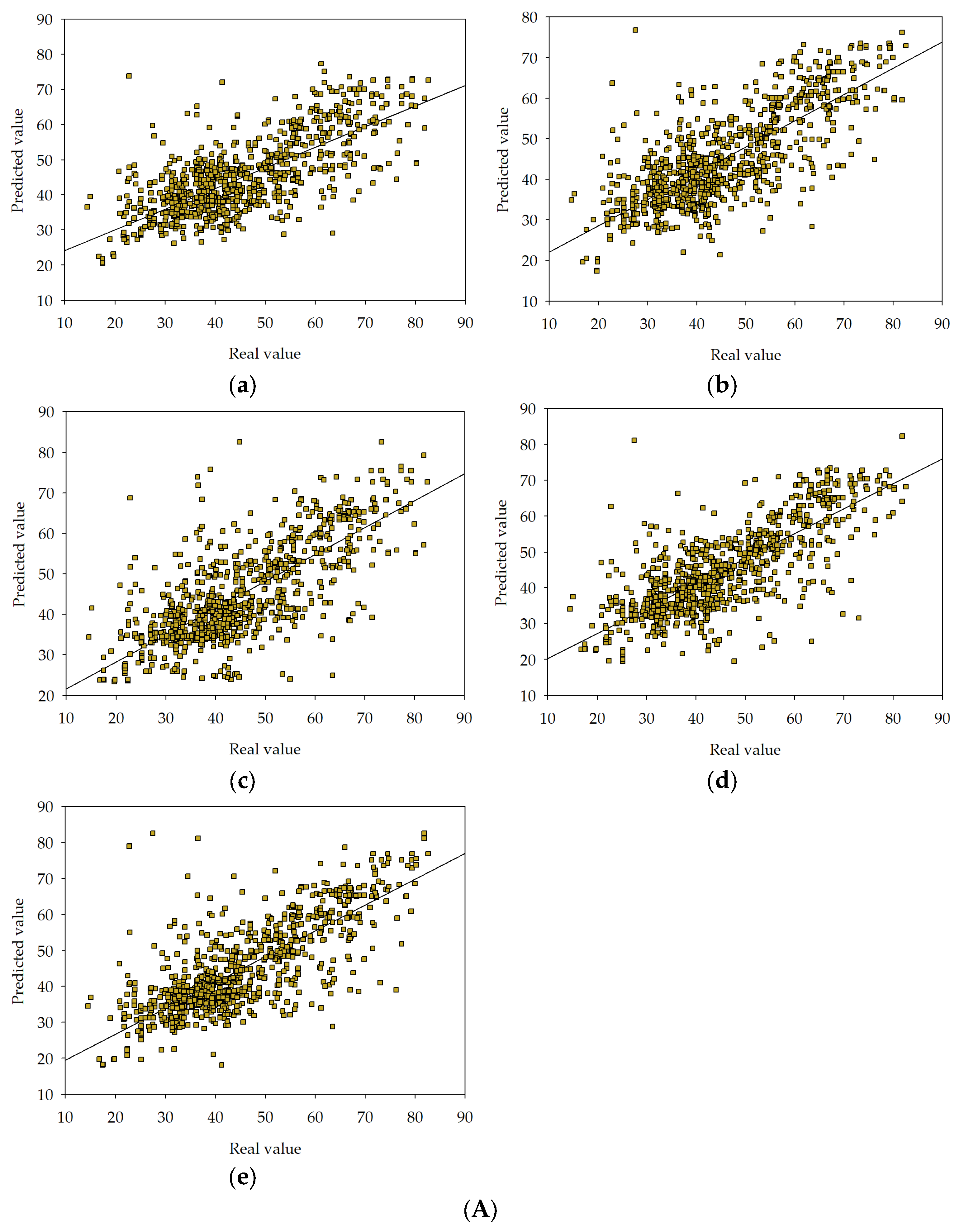
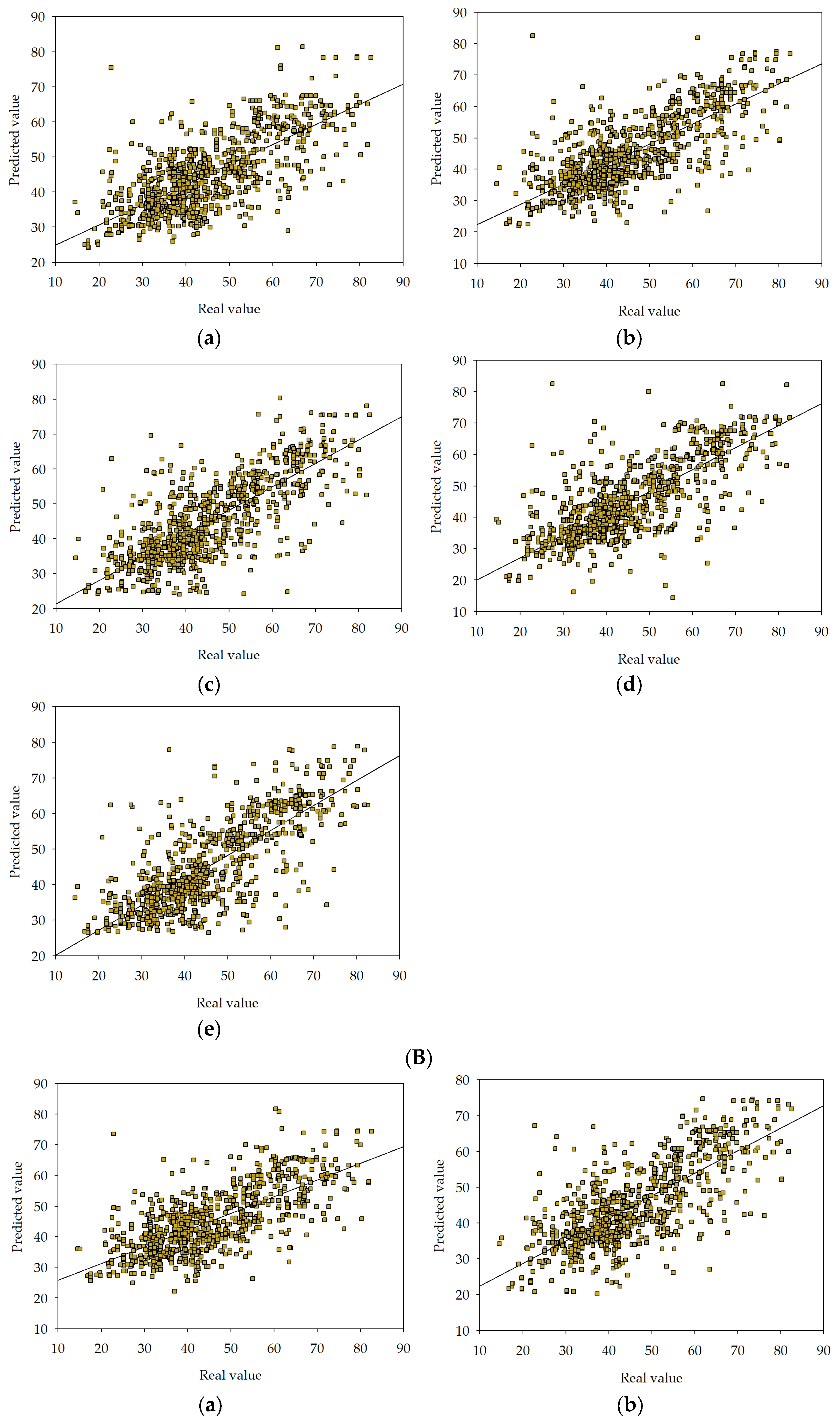
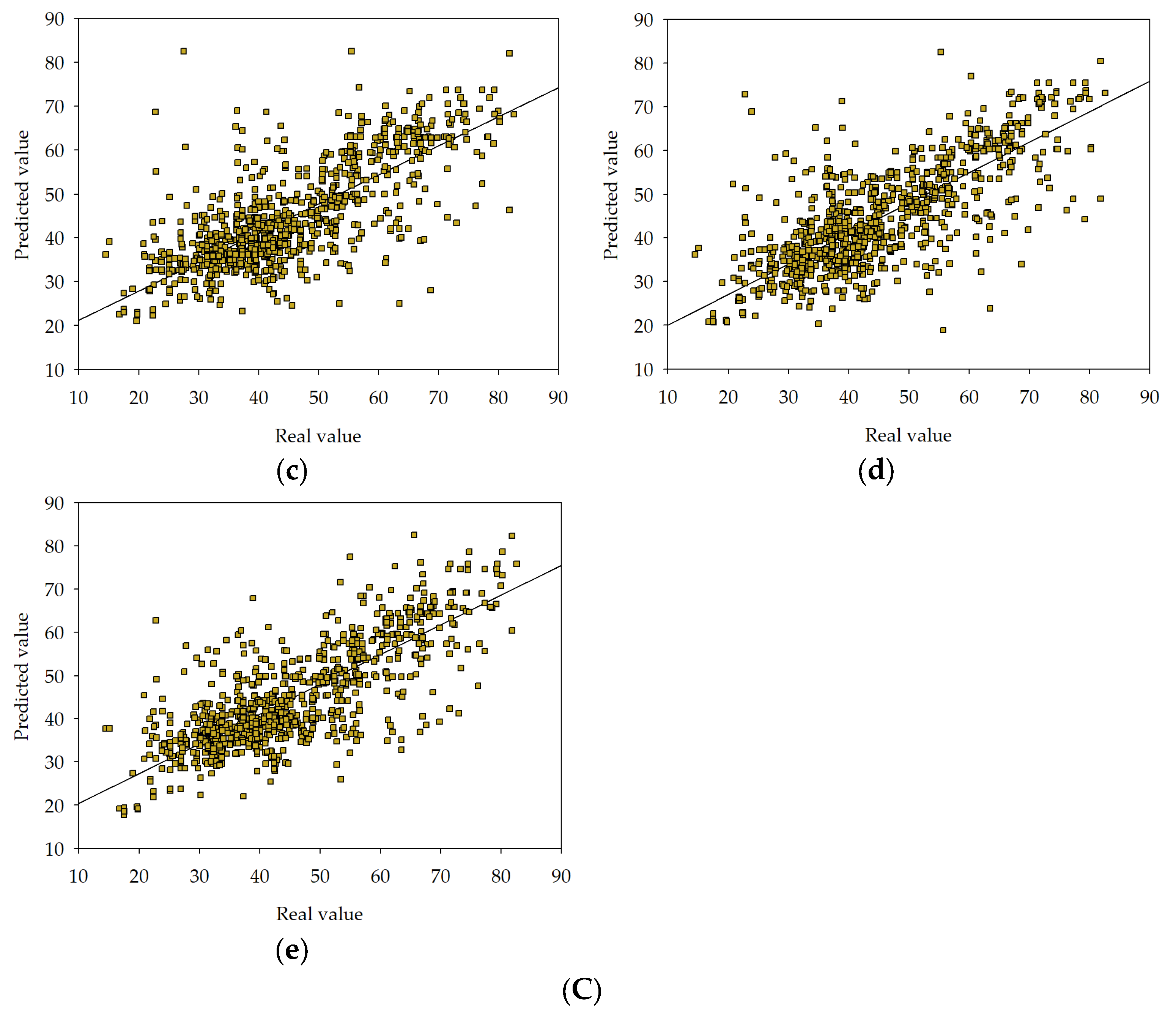
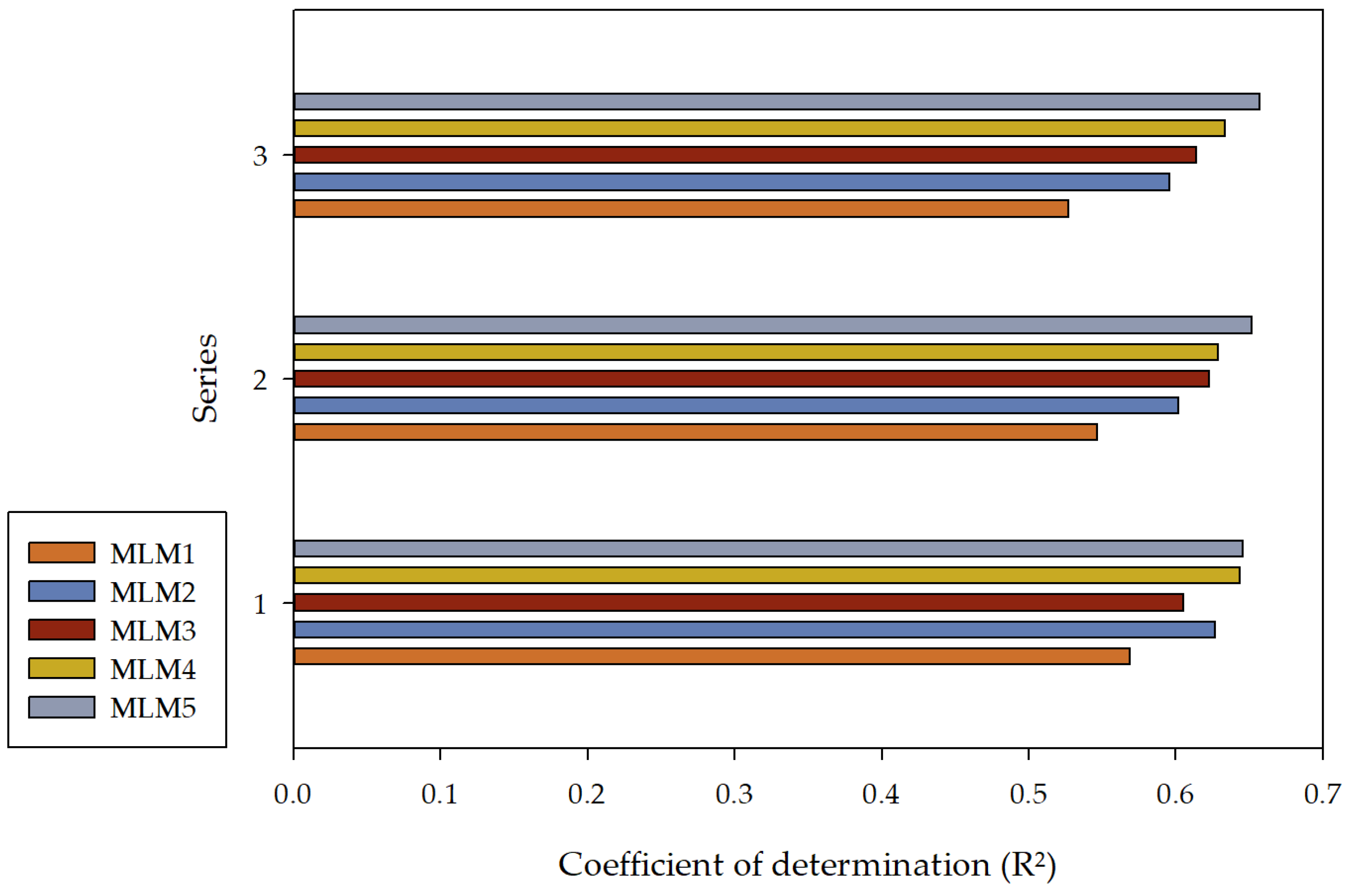
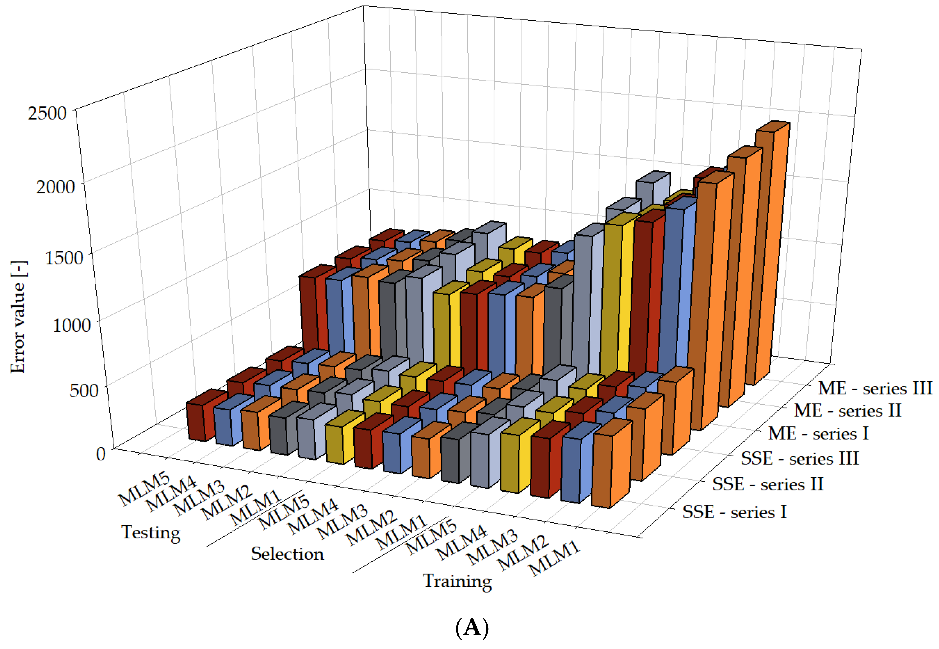
  in series I, II, and III.
, MLM2 , MLM3 , MLM4 , MLM5 in series I, II, and III.
in series I, II, and III.
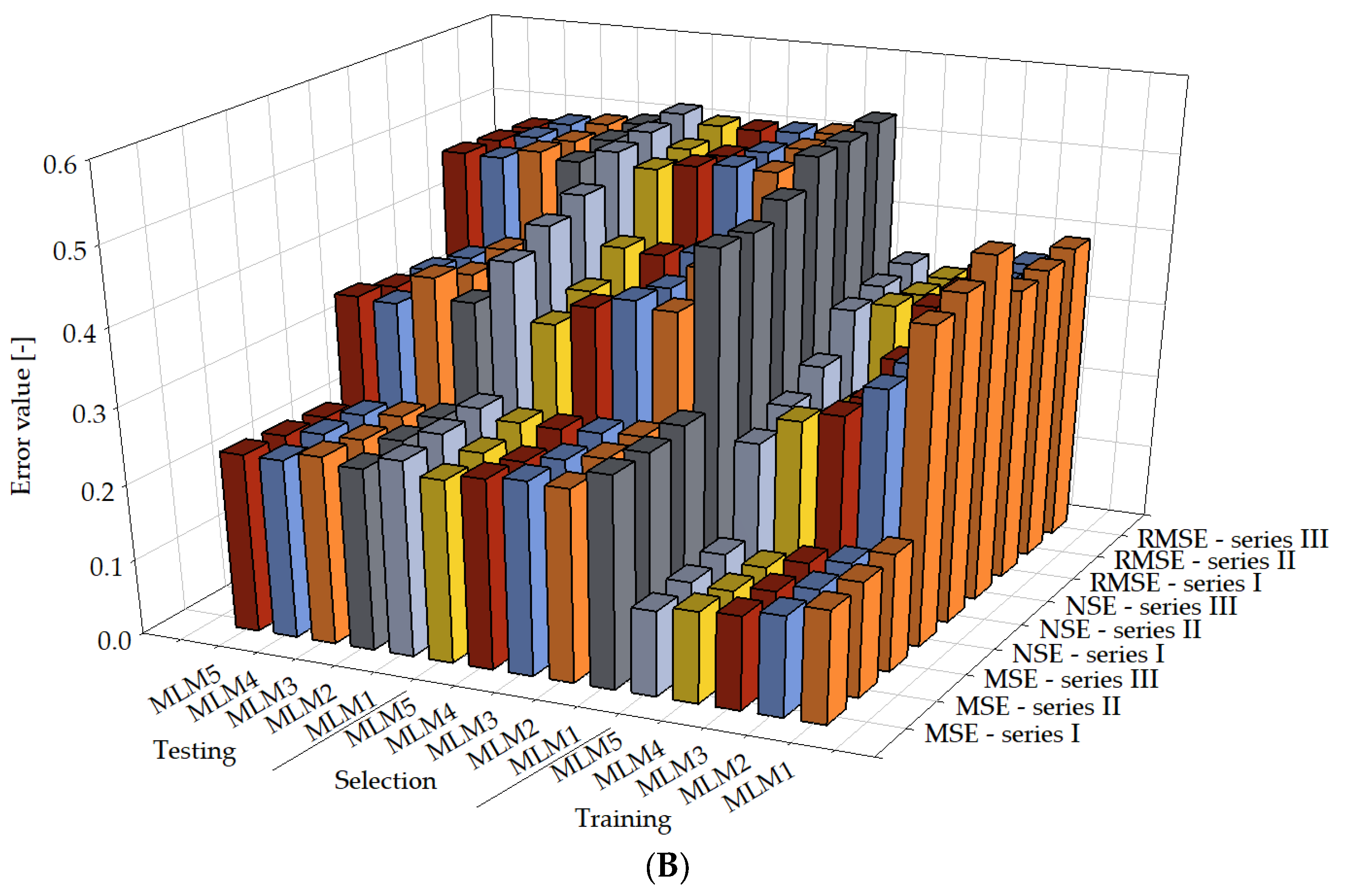
, MLM2 , MLM3 , MLM4 , MLM5 in series I, II, and III.


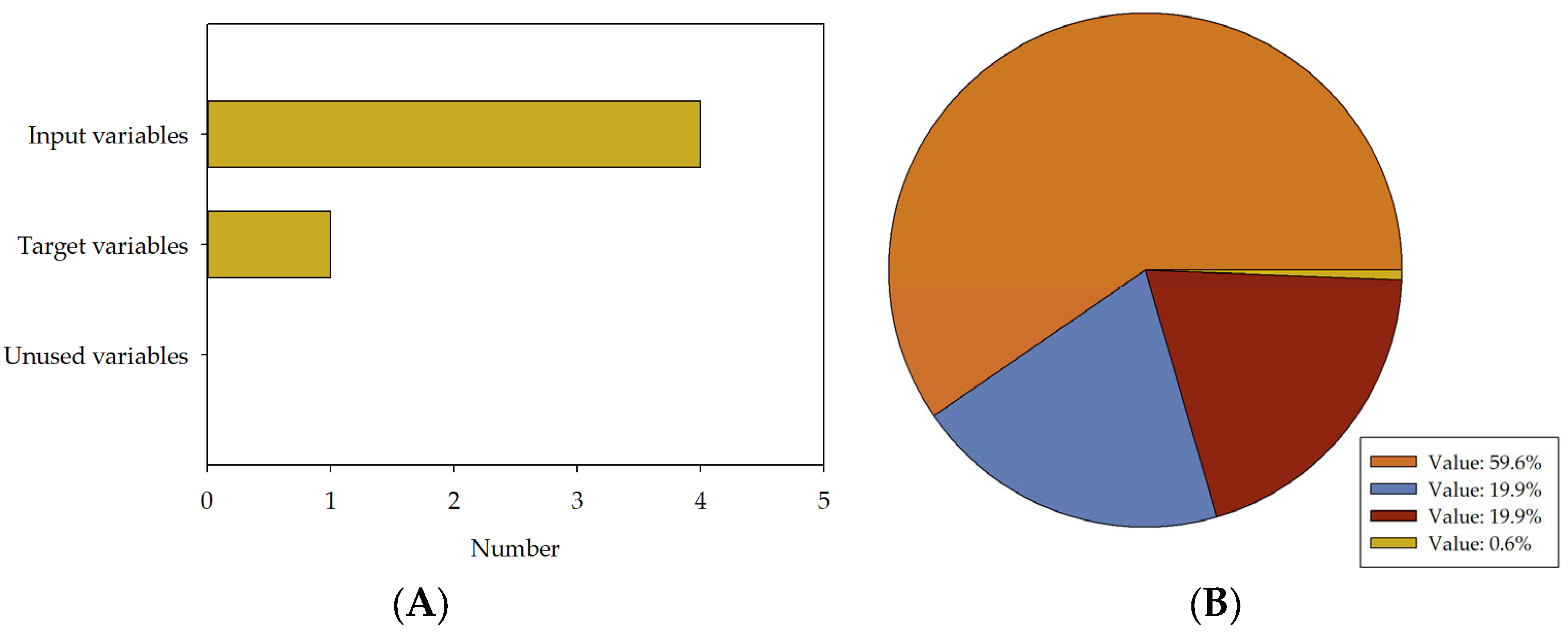
| Parameter | Concrete Compressive Strength | Cement | Water–Cement Ratio | Fine Aggregate | Coarse Aggregate |
|---|---|---|---|---|---|
| Type | Target | Input | Input | Input | Input |
| Description | The 28-day compressive strength of concrete that is considered to have most of its strength (MPa). | Content of cement added to the mixture (kg/m3). | Water-to-cement ratio (-). | Content of fine aggregate added to the mixture (kg/m3). | Content of coarse aggregate added to the mixture (kg/m3). |
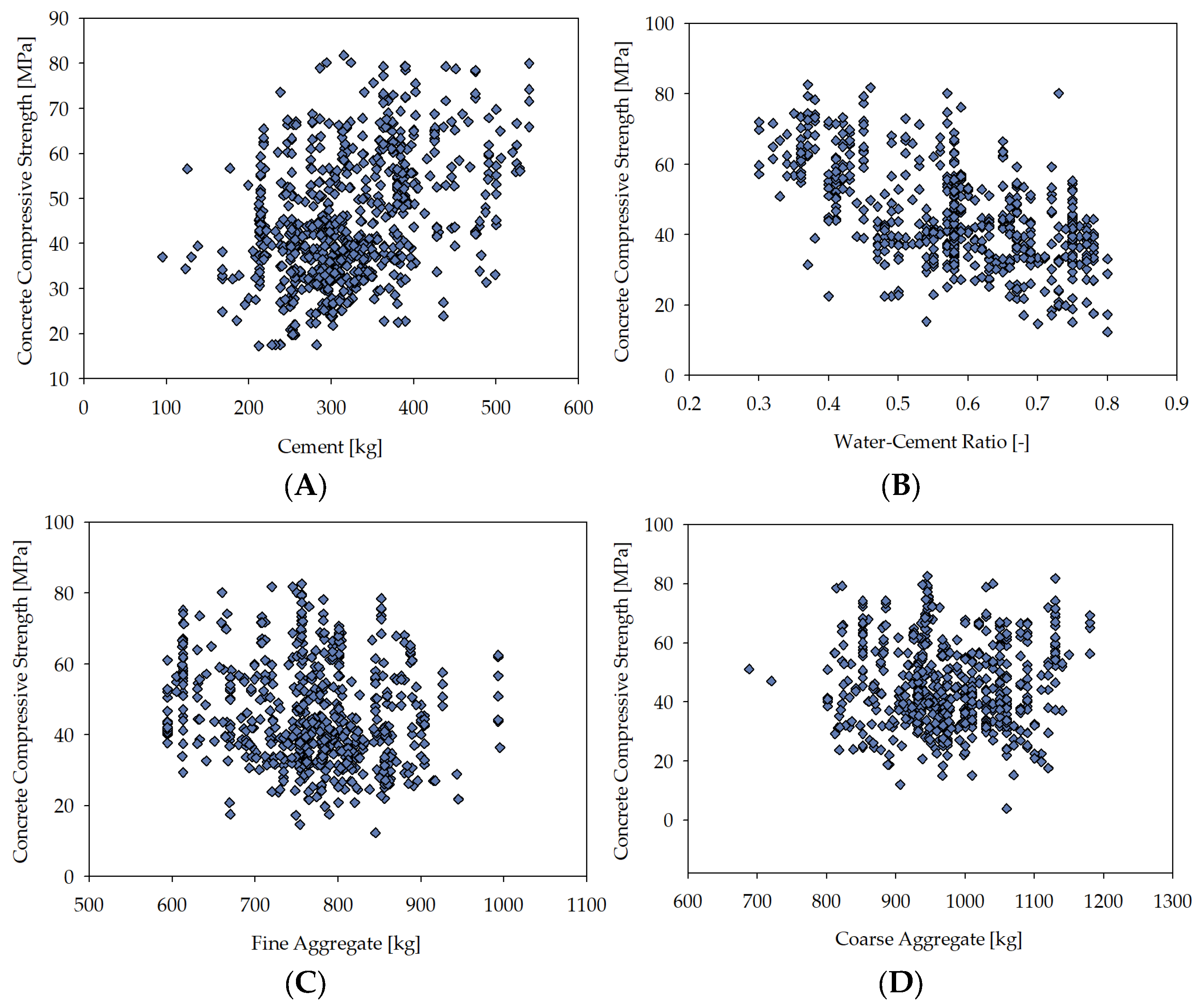
| Input Variable | Minimum | Maximum | Mean | Median | Dominant |
|---|---|---|---|---|---|
| Cement | 87.00 kg/m3 | 540.00 kg/m3 | 322.15 kg/m3 | 312.45 kg/m3 | 380.00 kg/m3 |
| Water–cement ratio | 0.30 | 0.80 | 0.58 | 0.58 | 0.58 |
| Fine aggregate | 472.00 kg/m3 | 995.60 kg/m3 | 767.96 kg/m3 | 774.00 kg/m3 | 594.00 kg/m3 |
| Coarse aggregate | 687.80 kg/m3 | 1198.00 kg/m3 | 969.92 kg/m3 | 963.00 kg/m3 | 932.00 kg/m3 |
| Series I | |||
| MLM1 | |||
| Training | Selection | Testing | |
| Sum squared error | 550.201 | 342.198 | 317.183 |
| Mean squared error | 0.149 | 0.278 | 0.258 |
| Root mean squared error | 0.386 | 0.528 | 0.508 |
| Normalised squared error | 0.416 | 0.479 | 0.432 |
| Minkowski error | 1893.670 | 975.049 | 911.882 |
| MLM2 | |||
| Training | Selection | Testing | |
| Sum squared error | 489.493 | 310.386 | 295.271 |
| Mean squared error | 0.133 | 0.253 | 0.240 |
| Root mean squared error | 0.364 | 0.503 | 0.490 |
| Normalised squared error | 0.330 | 0.394 | 0.374 |
| Minkowski error | 1680.550 | 876.432 | 842.034 |
| MLM3 | |||
| Training | Selection | Testing | |
| Sum squared error | 458.547 | 313.610 | 305.511 |
| Mean squared error | 0.124 | 0.255 | 0.248 |
| Root mean squared error | 0.353 | 0.505 | 0.498 |
| Normalised squared error | 0.289 | 0.402 | 0.400 |
| Minkowski error | 1561.140 | 865.786 | 860.635 |
| MLM4 | |||
| Training | Selection | Testing | |
| Sum squared error | 447.218 | 307.594 | 290.030 |
| Mean squared error | 0.121 | 0.250 | 0.236 |
| Root mean squared error | 0.348 | 0.500 | 0.485 |
| Normalised squared error | 0.275 | 0.387 | 0.361 |
| Minkowski error | 1510.870 | 842.743 | 807.330 |
| MLM5 | |||
| Training | Selection | Testing | |
| Sum squared error | 416.643 | 296.432 | 291.111 |
| Mean squared error | 0.113 | 0.241 | 0.236 |
| Root mean squared error | 0.336 | 0.491 | 0.486 |
| Normalised squared error | 0.239 | 0.359 | 0.364 |
| Minkowski error | 1403.290 | 810.031 | 798.990 |
| Series II | |||
| MLM1 | |||
| Training | Selection | Testing | |
| Sum squared error | 559.448 | 340.780 | 325.536 |
| Mean squared error | 0.152 | 0.277 | 0.264 |
| Root mean squared error | 0.389 | 0.527 | 0.514 |
| Normalised squared error | 0.431 | 0.475 | 0.455 |
| Minkowski error | 1944.850 | 974.611 | 947.078 |
| MLM2 | |||
| Training | Selection | Testing | |
| Sum squared error | 493.298 | 322.494 | 305.668 |
| Mean squared error | 0.134 | 0.262 | 0.248 |
| Root mean squared error | 0.366 | 0.512 | 0.498 |
| Normalised squared error | 0.335 | 0.425 | 0.401 |
| Minkowski error | 1687.480 | 905.087 | 867.447 |
| MLM3 | |||
| Training | Selection | Testing | |
| Sum squared error | 454.568 | 310.576 | 297.960 |
| Mean squared error | 0.123 | 0.253 | 0.242 |
| Root mean squared error | 0.351 | 0.503 | 0.492 |
| Normalised squared error | 0.284 | 0.394 | 0.381 |
| Minkowski error | 1539.040 | 852.571 | 837.393 |
| MLM4 | |||
| Training | Selection | Testing | |
| Sum squared error | 423.191 | 298.929 | 297.827 |
| Mean squared error | 0.115 | 0.243 | 0.242 |
| Root mean squared error | 0.339 | 0.493 | 0.492 |
| Normalised squared error | 0.246 | 0.365 | 0.381 |
| Minkowski error | 1431.560 | 823.304 | 820.941 |
| MLM5 | |||
| Training | Selection | Testing | |
| Sum squared error | 435.508 | 304.092 | 286.750 |
| Mean squared error | 0.118 | 0.247 | 0.233 |
| Root mean squared error | 0.344 | 0.497 | 0.483 |
| Normalised squared error | 0.261 | 0.378 | 0.353 |
| Minkowski error | 1458.890 | 834.351 | 799.642 |
| Series III | |||
| MLM1 | |||
| Training | Selection | Testing | |
| Sum squared error | 575.272 | 347.520 | 332.199 |
| Mean squared error | 0.156 | 0.283 | 0.270 |
| Root mean squared error | 0.395 | 0.532 | 0.519 |
| Normalised squared error | 0.455 | 0.494 | 0.473 |
| Minkowski error | 2007.800 | 1004.980 | 969.083 |
| MLM2 | |||
| Training | Selection | Testing | |
| Sum squared error | 500.105 | 321.972 | 307.902 |
| Mean squared error | 0.136 | 0.262 | 0.250 |
| Root mean squared error | 0.368 | 0.512 | 0.500 |
| Normalised squared error | 0.344 | 0.424 | 0.407 |
| Minkowski error | 1706.130 | 905.095 | 879.370 |
| MLM3 | |||
| Training | Selection | Testing | |
| Sum squared error | 473.081 | 318.669 | 301.983 |
| Mean squared error | 0.128 | 0.259 | 0.245 |
| Root mean squared error | 0.358 | 0.509 | 0.495 |
| Normalised squared error | 0.308 | 0.415 | 0.391 |
| Minkowski error | 1608.550 | 889.350 | 844.676 |
| MLM4 | |||
| Training | Selection | Testing | |
| Sum squared error | 419.356 | 315.651 | 295.121 |
| Mean squared error | 0.114 | 0.257 | 0.240 |
| Root mean squared error | 0.337 | 0.507 | 0.490 |
| Normalised squared error | 0.242 | 0.407 | 0.374 |
| Minkowski error | 1407.230 | 862.350 | 814.506 |
| MLM5 | |||
| Training | Selection | Testing | |
| Sum squared error | 455.535 | 317.058 | 283.630 |
| Mean squared error | 0.123 | 0.258 | 0.230 |
| Root mean squared error | 0.351 | 0.508 | 0.480 |
| Normalised squared error | 0.286 | 0.411 | 0.345 |
| Minkowski error | 1529.650 | 866.807 | 798.284 |
| Series I | ||||
| Minimum | Maximum | Mean | Deviation | |
| Absolute error | ||||
| MLM1 | 0.00000119209 | 0.0695368 | 0.00936655 | 0.00818558 |
| MLM2 | 0.00000104308 | 0.0120825 | 0.00145332 | 0.00118896 |
| MLM3 | 0.000000119209 | 0.0879388 | 0.00273278 | 0.0041617 |
| MLM4 | 0.00000119209 | 0.148637 | 0.00331478 | 0.00663424 |
| MLM5 | 0.00000119209 | 0.148637 | 0.00331478 | 0.00663424 |
| Relative error | ||||
| MLM1 | 0.0000011413 | 0.0665743 | 0.00896749 | 0.00783684 |
| MLM2 | 0.00000851071 | 0.0985832 | 0.011858 | 0.009701 |
| MLM3 | 0.000000296304 | 0.218579 | 0.00679255 | 0.0103442 |
| MLM4 | 0.00000213266 | 0.265913 | 0.00593016 | 0.0118687 |
| MLM5 | 0.00000119209 | 0.148637 | 0.00331478 | 0.00663424 |
| Percentage error | ||||
| MLM1 | 0.00011413 | 6.65743 | 0.896749 | 0.783684 |
| MLM2 | 0.000851071 | 9.85832 | 1.1858 | 0.9701 |
| MLM3 | 0.0000296304 | 21.8579 | 0.679255 | 1.03442 |
| MLM4 | 0.000213266 | 26.5913 | 0.593016 | 1.18687 |
| MLM5 | 0.00000119209 | 0.148637 | 0.00331478 | 0.00663424 |
| Series II | ||||
| Minimum | Maximum | Mean | Deviation | |
| Absolute error | ||||
| MLM1 | 0.00000119209 | 0.0695368 | 0.00936655 | 0.00818558 |
| MLM2 | 0.00000104308 | 0.0120825 | 0.00145332 | 0.00118896 |
| MLM3 | 0.000000119209 | 0.0879388 | 0.00273278 | 0.0041617 |
| MLM4 | 0.00000119209 | 0.148637 | 0.00331478 | 0.00663424 |
| MLM5 | 0.00000119209 | 0.148637 | 0.00331478 | 0.00663424 |
| Relative error | ||||
| MLM1 | 0.0000011413 | 0.0665743 | 0.00896749 | 0.00783684 |
| MLM2 | 0.00000851071 | 0.0985832 | 0.011858 | 0.009701 |
| MLM3 | 0.000000296304 | 0.218579 | 0.00679255 | 0.0103442 |
| MLM4 | 0.00000213266 | 0.265913 | 0.00593016 | 0.0118687 |
| MLM5 | 0.00000119209 | 0.148637 | 0.00331478 | 0.00663424 |
| Percentage error | ||||
| MLM1 | 0.00011413 | 6.65743 | 0.896749 | 0.783684 |
| MLM2 | 0.000851071 | 9.85832 | 1.1858 | 0.9701 |
| MLM3 | 0.0000296304 | 21.8579 | 0.679255 | 1.03442 |
| MLM4 | 0.000213266 | 26.5913 | 0.593016 | 1.18687 |
| MLM5 | 0.00000119209 | 0.148637 | 0.00331478 | 0.00663424 |
| Series III | ||||
| Minimum | Maximum | Mean | Deviation | |
| Absolute error | ||||
| MLM1 | 0.00000119209 | 0.0695368 | 0.00936655 | 0.00818558 |
| MLM2 | 0.00000104308 | 0.0120825 | 0.00145332 | 0.00118896 |
| MLM3 | 0.000000119209 | 0.0879388 | 0.00273278 | 0.0041617 |
| MLM4 | 0.00000119209 | 0.148637 | 0.00331478 | 0.00663424 |
| MLM5 | 0.00000119209 | 0.148637 | 0.00331478 | 0.00663424 |
| Relative error | ||||
| MLM1 | 0.0000011413 | 0.0665743 | 0.00896749 | 0.00783684 |
| MLM2 | 0.00000851071 | 0.0985832 | 0.011858 | 0.009701 |
| MLM3 | 0.000000296304 | 0.218579 | 0.00679255 | 0.0103442 |
| MLM4 | 0.00000213266 | 0.265913 | 0.00593016 | 0.0118687 |
| MLM5 | 0.00000119209 | 0.148637 | 0.00331478 | 0.00663424 |
| Percentage error | ||||
| MLM1 | 0.00011413 | 6.65743 | 0.896749 | 0.783684 |
| MLM2 | 0.000851071 | 9.85832 | 1.1858 | 0.9701 |
| MLM3 | 0.0000296304 | 21.8579 | 0.679255 | 1.03442 |
| MLM4 | 0.000213266 | 26.5913 | 0.593016 | 1.18687 |
| MLM5 | 0.00000119209 | 0.148637 | 0.00331478 | 0.00663424 |
Disclaimer/Publisher’s Note: The statements, opinions and data contained in all publications are solely those of the individual author(s) and contributor(s) and not of MDPI and/or the editor(s). MDPI and/or the editor(s) disclaim responsibility for any injury to people or property resulting from any ideas, methods, instructions or products referred to in the content. |
© 2023 by the author. Licensee MDPI, Basel, Switzerland. This article is an open access article distributed under the terms and conditions of the Creative Commons Attribution (CC BY) license (https://creativecommons.org/licenses/by/4.0/).
Share and Cite
Ziolkowski, P. Computational Complexity and Its Influence on Predictive Capabilities of Machine Learning Models for Concrete Mix Design. Materials 2023, 16, 5956. https://doi.org/10.3390/ma16175956
Ziolkowski P. Computational Complexity and Its Influence on Predictive Capabilities of Machine Learning Models for Concrete Mix Design. Materials. 2023; 16(17):5956. https://doi.org/10.3390/ma16175956
Chicago/Turabian StyleZiolkowski, Patryk. 2023. "Computational Complexity and Its Influence on Predictive Capabilities of Machine Learning Models for Concrete Mix Design" Materials 16, no. 17: 5956. https://doi.org/10.3390/ma16175956