
A Constitutive Model for Describing the Tensile Response of Woven Polyethylene Terephthalate Geogrids after Damage

 , and
, and
Abstract
:1. Introduction
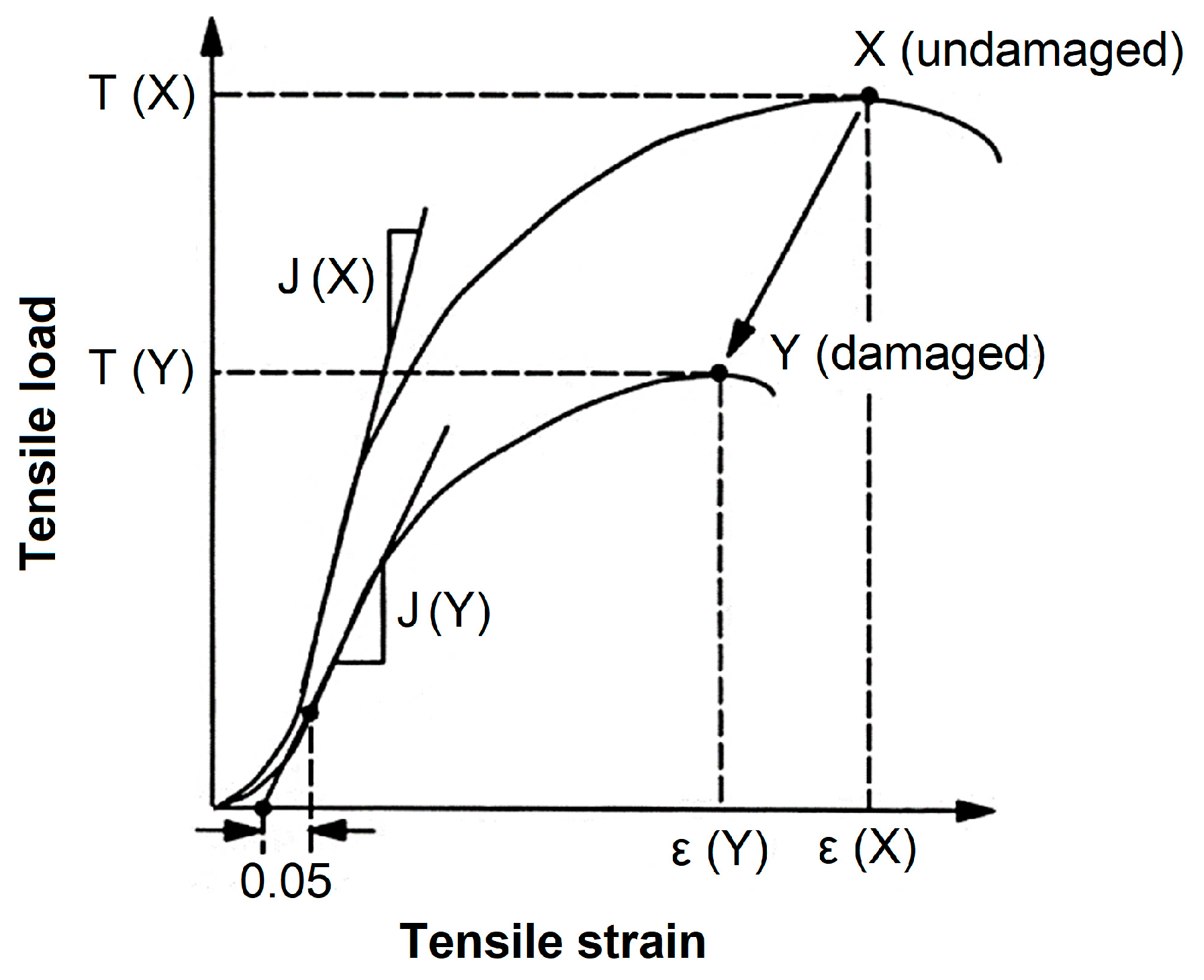
- T: tensile load per unit width;
- J: tangent stiffness;
- ε: tensile strain;
- a, b, and c: model parameters;
- εmax: strain at maximum load.
- RT, RJ and Rε: scaling factors;
- X: undamaged sample;
- Y: damaged sample.
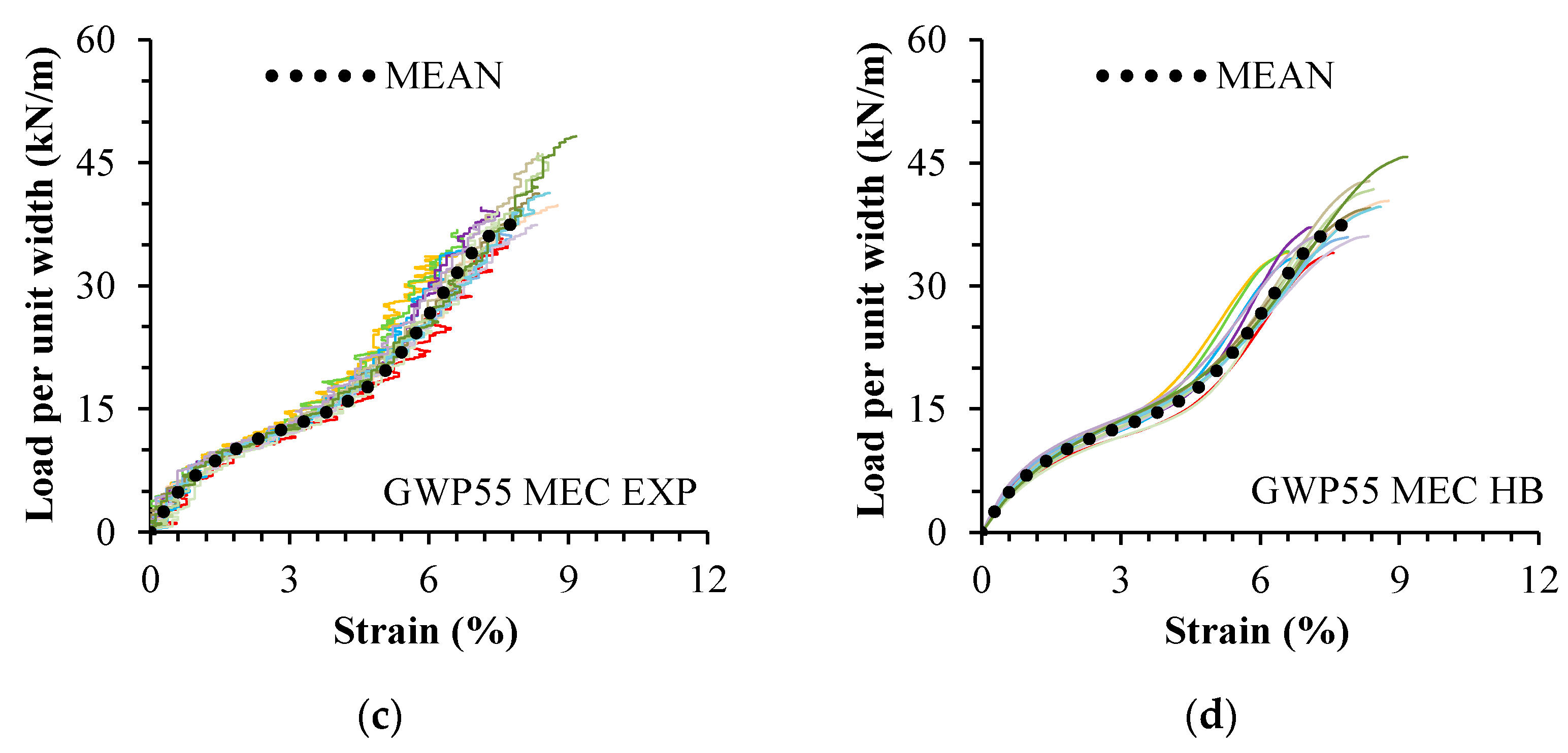
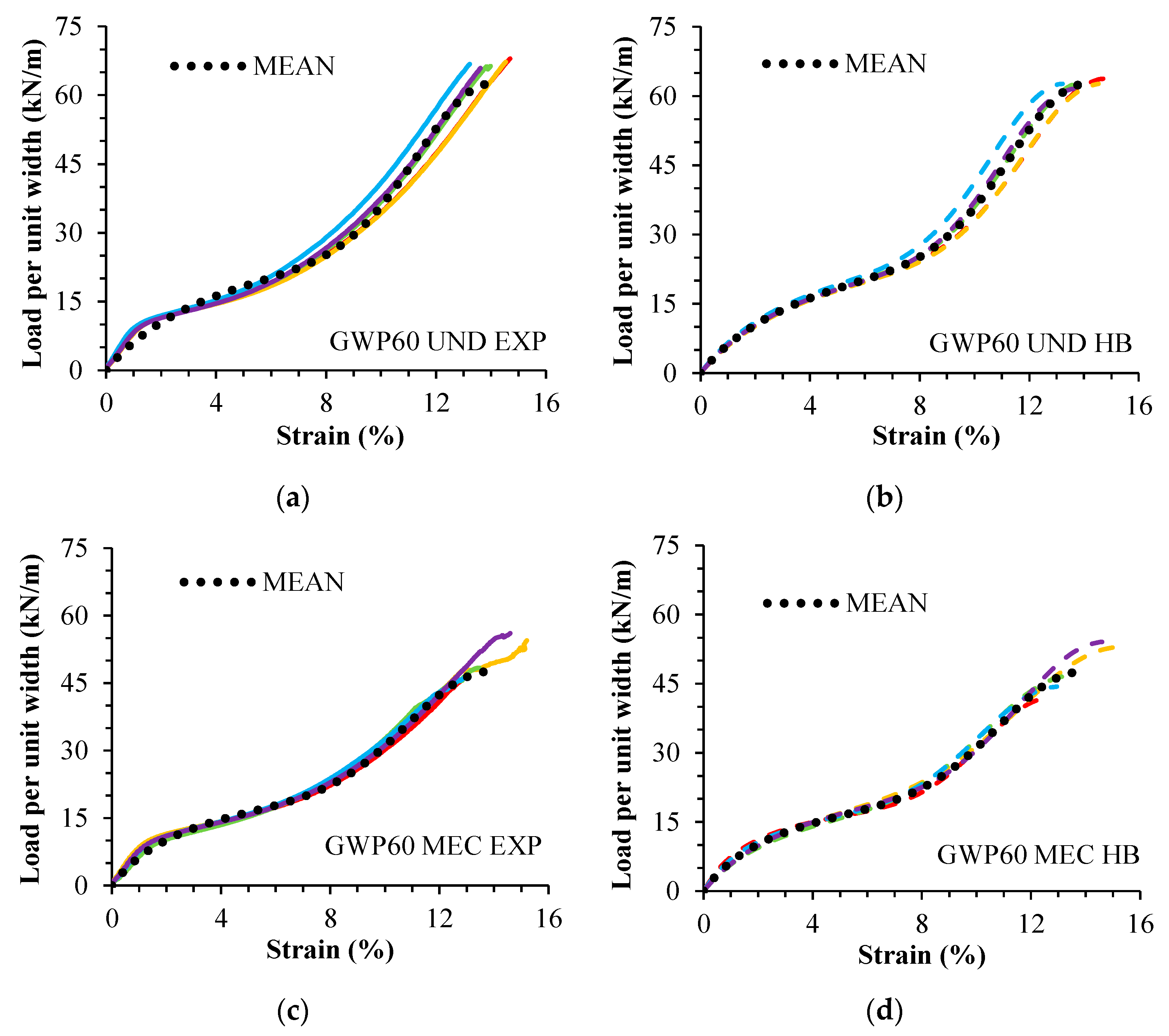
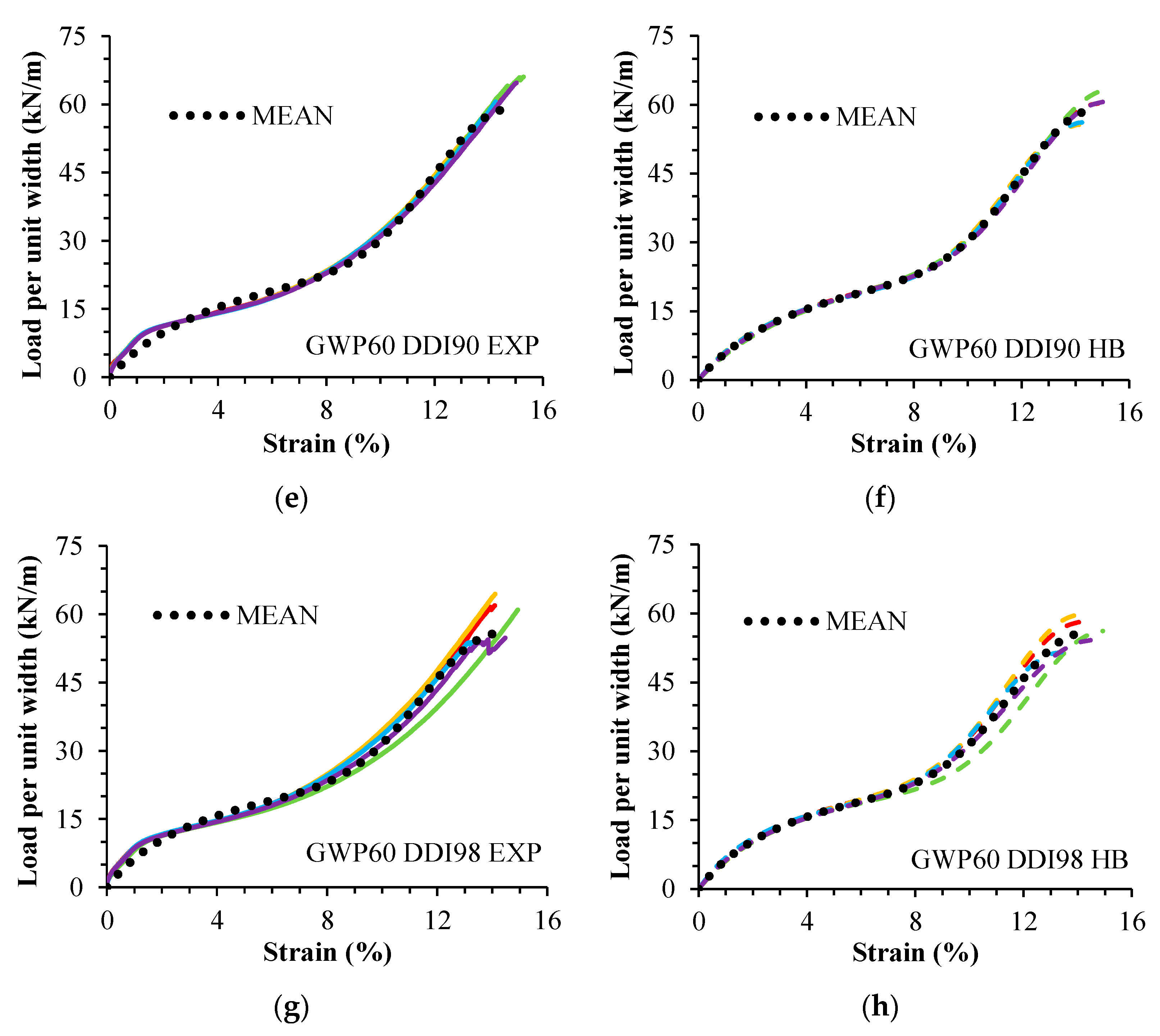
- Apply a constitutive model to describe the short-term tensile response of undamaged and damaged specimens of two woven Polyethylene Terephthalate (PET) geogrids; estimate the model parameters; assess the goodness of the fits; statistically compare experimental and fitted data.
- Determine the scaling factors by relating the tensile properties of undamaged and damaged samples of the geogrids.
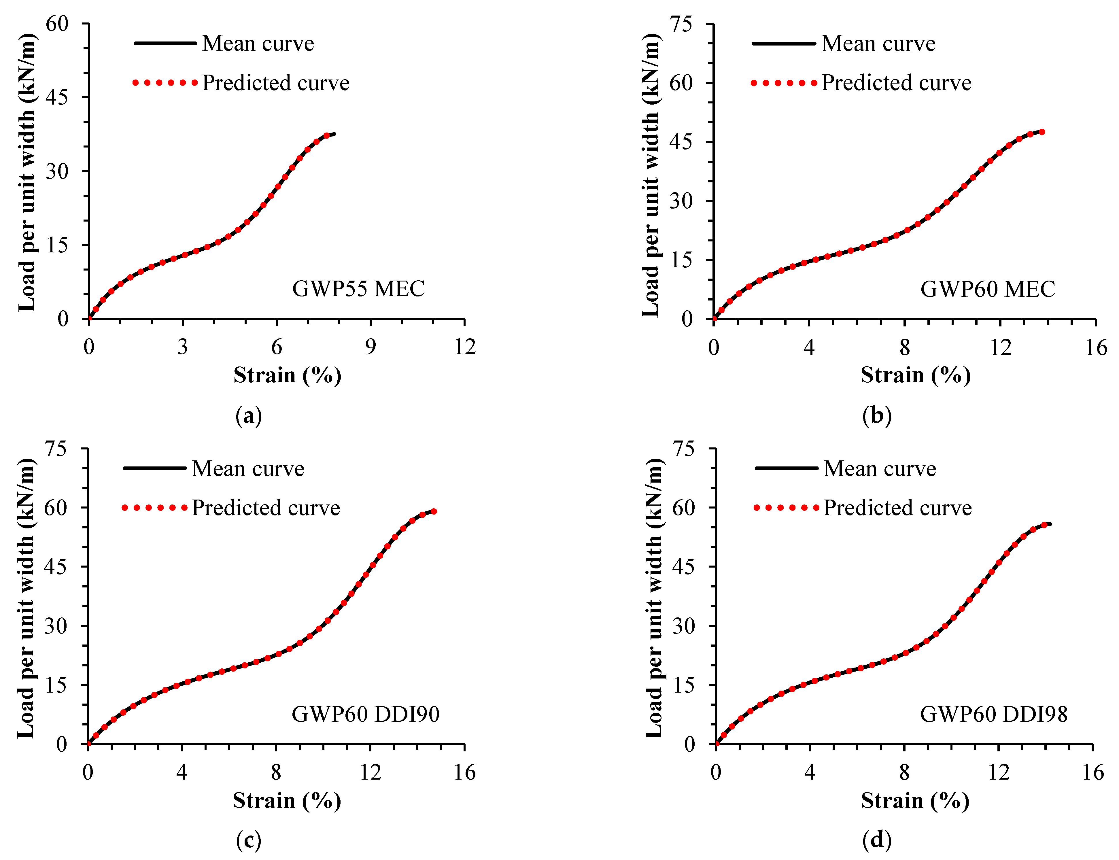
- For each geogrid, obtain the tensile load–strain curve of damaged samples by applying scaling factors to the plot of the undamaged sample; assess the goodness of the fits; statistically compare predicted and fitted data.
2. Materials
3. Methods
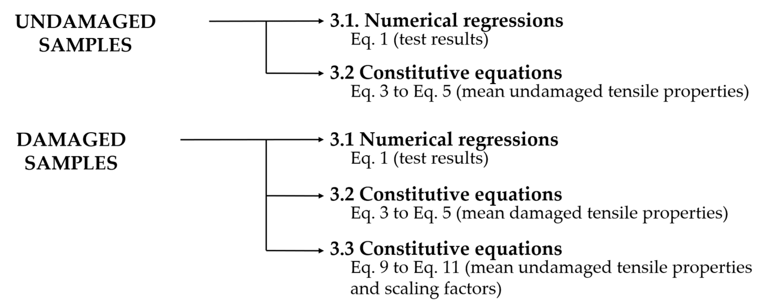
3.1. Numerical Regressions (Curve Fittings)
3.2. Mathematical Relations between the Model Parameters and the Tensile Properties
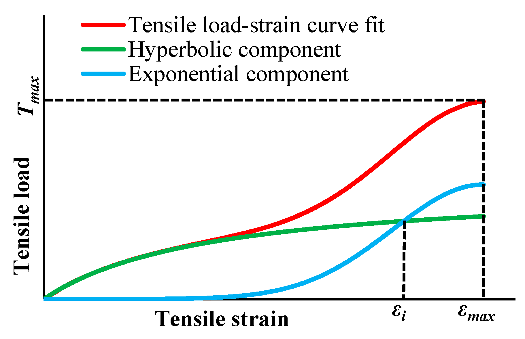
- Ji: initial tangent stiffness;
- Tmax: tensile strength;
- εi: strain for which the hyperbolic and exponential components intersect (Figure 1).
3.3. Damaged Curves Described Using Undamaged Data and Scaling Factors
4. Results and Discussions
5. Conclusions
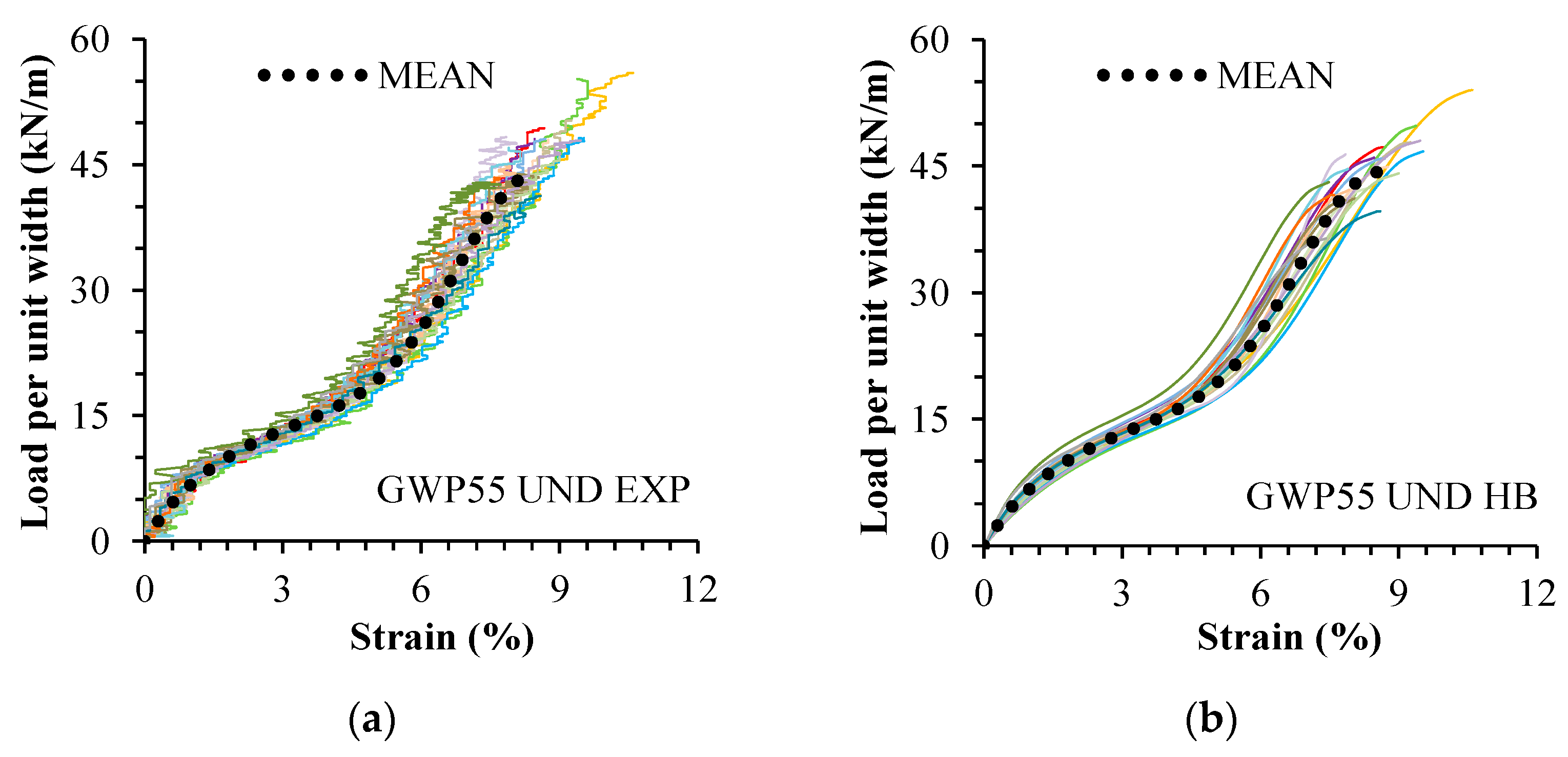
- The model was able to qualitatively describe the tensile load–strain response of undamaged and damaged specimens of both geogrids (high R2 values).
- If compared to experimental values, the model proved capable of fitting the tensile strength of most samples of the geogrids (for most samples, there was no significant mean difference between the experimental and fitted tensile strength).
- The model allowed us to describe the tensile load–strain curve of a geogrid (before and after damage) only from its tensile properties: , and .
- Regardless of the type of damage, the model was able to describe tensile load–strain curves of damaged samples using data from undamaged samples and scaling factors.
Author Contributions
Funding
Institutional Review Board Statement
Informed Consent Statement
Data Availability Statement
Conflicts of Interest
References
- ISO 10318-1; Geosynthetics—Part 1: Terms and Definitions. International Organization for Standardization: Geneva, Switzerland, 2015.
- Koerner, R.M. Designing with Geosynthetics, 5th ed.; Pearson Prentice Hall: Upper Saddle River, NJ, USA, 2005. [Google Scholar]
- Touze, N. Healing the World: A Geosynthetics Solution. Geosynth. Int. 2021, 28, 1–31. [Google Scholar] [CrossRef]
- Keller, G.R. Application of Geosynthetics on Low-Volume Roads. Transp. Geotech. 2016, 8, 119–131. [Google Scholar] [CrossRef]
- Giroud, J.P.; Han, J.; Tutumluer, E.; Dobie, M.J.D. The Use of Geosynthetics in Roads. Geosynth. Int. 2023, 30, 47–80. [Google Scholar] [CrossRef]
- Wang, C.; Luan, M.; Zhu, Z. Model Test and Numerical Analysis on Long-Term Mechanical Properties of Stepped Reinforced Retaining Wall. Trans. Tianjin Univ. 2012, 18, 62–68. [Google Scholar] [CrossRef]
- Zou, C.; Wang, Y.; Lin, J.; Chen, Y. Creep Behaviors and Constitutive Model for High Density Polyethylene Geogrid and Its Application to Reinforced Soil Retaining Wall on Soft Soil Foundation. Constr. Build. Mater. 2016, 114, 763–771. [Google Scholar] [CrossRef]
- Adams, M.; Nicks, J. Design and Construction Guidelines for Geosynthetic Reinforced Soil Abutments and Integrated Bridge Systems; FHWA-HRT-17-080; Federal Highway Administration: St Paul, MN, USA, 2018.
- Gao, W.; Kavazanjian, E.; Wu, X. Numerical Study of Strain Development in High-Density Polyethylene Geomembrane Liner System in Landfills Using a New Constitutive Model for Municipal Solid Waste. Geotext. Geomembr. 2022, 50, 216–230. [Google Scholar] [CrossRef]
- Cen, W.J.; Bauer, E.; Wen, L.S.; Wang, H.; Sun, Y.J. Experimental Investigations and Constitutive Modeling of Cyclic Interface Shearing between HDPE Geomembrane and Sandy Gravel. Geotext. Geomembr. 2019, 47, 269–279. [Google Scholar] [CrossRef]
- Bacas, B.M.; Konietzky, H.; Berini, J.C.; Sagaseta, C. A New Constitutive Model for Textured Geomembrane/Geotextile Interfaces. Geotext. Geomembr. 2011, 29, 137–148. [Google Scholar] [CrossRef]
- Zarnani, S.; Bathurst, R.J. Influence of Constitutive Model on Numerical Simulation of EPS Seismic Buffer Shaking Table Tests. Geotext. Geomembr. 2009, 27, 308–312. [Google Scholar] [CrossRef]
- Ottosen, N.; Ristinmaa, M. The Mechanics of Constitutive Modeling; Elsevier Ltd.: Edinburgh, UK, 2005; ISBN 9780080446066. [Google Scholar]
- McGown, A.; Khan, A.J.; Kupec, J. The Isochronous Strains Energy Approach Applied to the Load-Strain-Time-Temperature Behaviour of Geosynthetics. Geosynth. Int. 2004, 11, 114–130. [Google Scholar] [CrossRef]
- Shukla, S.K. An Introduction to Geosynthetic Engineering; CRC Press: Leiden, The Netherlands, 2016; ISBN 9781138027749. [Google Scholar]
- Bathurst, R.J.; Kaliakin, V.N. Review of Numerical Models for Geosynthetics in Reinforcement Applications. In Proceedings of the 11th International Conference of the International Association for Computer Methods and Advances in Geomechanics, Torino, Italy, 19–24 June 2005; Volume 4, pp. 407–416. [Google Scholar]
- Yogendrakumar, K.; Bathurst, R.J. Numerical Simulation of Reinforced Soil Structure During Blast Loads. Transp. Res. Rec. 1992, 1336, 1–8. [Google Scholar]
- Ling, H.I.; Tatsuoka, F.; Tateyama, M. Simulating Performance of GRS-RW by Finite-Element Procedure. J. Geotech. Eng. 1995, 121, 330–340. [Google Scholar] [CrossRef]
- Liu, H.; Ling, H.I. Modeling Cyclic Behavior of Geosynthetics Using Mathematical Functions Combined with Masing Rule and Bounding Surface Plasticity. Geosynth. Int. 2006, 13, 234–245. [Google Scholar] [CrossRef]
- Zhou, Z.G.; Li, Y.Z. Creep Properties and Viscoelastic-Plastic-Damaged Constitutive Model of Geogrid. Chin. J. Geotech. Eng. 2011, 33, 1943–1949. [Google Scholar]
- Haimin, W.; Yiming, S.; Linjun, D.; Zhaoming, T. Implementation and Verification of a Geosynthetic-Soil Interface Constitutive Model in the Geogrid Element of FLAC3D. Acta Geotech. Slov. 2015, 12, 27–35. [Google Scholar]
- Paula, A.M.; Pinho-Lopes, M. Constitutive Modelling of Short-Term Tensile Response of Geotextile Subjected to Mechanical and Abrasion Damages. Int. J. Geosynth. Ground Eng. 2021, 7, 1–11. [Google Scholar] [CrossRef]
- Lombardi, G.; Paula, A.M.; Pinho-Lopes, M. Constitutive Models and Statistical Analysis of the Short-Term Tensile Response of Geosynthetics after Damage. Constr. Build. Mater. 2022, 317, 125972. [Google Scholar] [CrossRef]
- Ding, L.; Xiao, C.; Cui, F. Analytical Model for Predicting Time-Dependent Lateral Deformation of Geosynthetics-Reinforced Soil Walls with Modular Block Facing. J. Rock Mech. Geotech. Eng. 2023. [Google Scholar] [CrossRef]
- Bathurst, R.J.; Naftchali, F.M. Geosynthetic Reinforcement Stiffness for Analytical and Numerical Modelling of Reinforced Soil Structures. Geotext. Geomembr. 2021, 49, 921–940. [Google Scholar] [CrossRef]
- Ezzein, F.M.; Bathurst, R.J.; Kongkitkul, W. Nonlinear Load–Strain Modeling of Polypropylene Geogrids during Constant Rate-of-Strain Loading. Polym. Eng. Sci. 2015, 55, 1617–1627. [Google Scholar] [CrossRef]
- Greenwood, J.H.; Schroeder, H.F.; Voskamp, W. Durability of Geosynthetics; CUR Building & Infrastructure: Gouda, The Netherlands, 2012; ISBN 9789037605334. [Google Scholar]
- Allen, T.M.; Bathurst, R.J. Characterization of Geosynthetic Load-Strain Behavior After Installation Damage. Geosynth. Int. 1994, 1, 181–199. [Google Scholar] [CrossRef]
- ISO 10722; Geosynthetics—Index Test Procedure for the Evaluation of Mechanical Damage under Repeated Loading—Damage Caused by Granular Material. International Organization for Standardization: Geneva, Switzerland, 2019.
- Rosete, A.; Mendonça Lopes, P.; Pinho-Lopes, M.; Lopes, M.L. Tensile and Hydraulic Properties of Geosynthetics after Mechanical Damage and Abrasion Laboratory Tests. Geosynth. Int. 2013, 20, 358–374. [Google Scholar] [CrossRef] [Green Version]
- Pinho-Lopes, M.; Lopes, M.L. Synergisms between Laboratory Mechanical and Abrasion Damage on Mechanical and Hydraulic Properties of Geosynthetics. Transp. Geotech. 2015, 4, 50–63. [Google Scholar] [CrossRef] [Green Version]
- Pinho-Lopes, M.; Recker, C.; Lopes, M.L.; Müller-Rochholz, J. Experimental Analysis of the Combined Effect of Installation Damage and Creep of Geosynthetics—New Results. In Proceedings of the 7th International Conference on Geosynthetics, Nice, France, 22–27 September 2002; Volume 4, pp. 1539–1544. [Google Scholar]
- ISO 10319; Geosynthetics—Wide-Width Tensile Test. International Organization for Standardization: Geneva, Switzerland, 2015.
- Sheskin, D.J. Handbook of Parametric and Non Parametric Statistical Procedures, 3rd ed.; Chapman & Hall/CRC: Boca Raton, FL, USA, 2000; ISBN 9781420036268. [Google Scholar]
- Field, A. Discovering Statistics Using SPSS, 5th ed.; SAGE Publications Ltd.: London, UK, 2017; ISBN 1847879071, 9781847879073. [Google Scholar]


| Geosynthetic | GWP55 | GWP60 | ||
|---|---|---|---|---|
| Type | Geogrid |  | Geogrid |  |
| Structure | Woven | Woven | ||
| Constituent polymer | PET | PET | ||
| Nominal tensile strength (kN/m) | 55 | 60 | ||
| Nominal tensile strain (%) | 10.5 | 14.0 | ||
| Grid spacing (mm × mm) | 25 × 25 | 20 × 20 | ||
| Term | Symbol | Definition |
|---|---|---|
| Model parameters | Parameters of the constitutive model (Equation (1)) | |
| Parameter estimates | – | Model parameters estimated via numerical regressions of experimental data |
| Mean parameter estimates | – | Mean estimates of the model parameter of a sample |
| Median parameter estimates | – | Median estimates of the model parameter of a sample |
| Tensile properties | Tensile properties of a certain geogrid | |
| Mean undamaged tensile properties | – | Mean experimental tensile properties of an undamaged sample |
| Mean damaged tensile properties | – | Mean experimental tensile properties of a damaged sample |
| Predicted damaged parameters | Model parameters for the response after damage predicted from undamaged data using scaling factors (Equations (3)–(5)) | |
| Representative curve: | – | Load–strain curve that best represents the trends in the data of a sample |
| – | Load–strain curve plotted using mean parameter estimates |
| – | Load–strain curve plotted using median parameter estimates |
| – | Experimental load–strain curve that visually is in an intermediate position relative to the other curves of a sample |
| Mean Experimental Tensile Properties | Mean Fitted Tensile Properties (Equation (1)) | |||
|---|---|---|---|---|
| Sample | εmax | Tmax | Tmax | Ji |
| % | kN/m | kN/m | kN/m | |
| GWP55 UND | 8.5 | 46.72 | 44.66 | 957.03 |
| GWP55 MEC | 7.8 | 39.80 | 37.88 | 938.93 |
| GWP60 UND | 14.0 | 66.84 | 62.70 * | 734.53 |
| GWP60 MEC | 13.8 | 50.11 | 48.16 | 744.54 |
| GWP60 DDI S90 | 14.7 | 63.01 | 59.19 | 708.04 |
| GWP60 DDI S98 | 14.2 | 59.23 | 55.99 | 786.16 |
| Sample | Mean Parameter Estimates | Tensile Properties | Scaling Factors | ||||||
|---|---|---|---|---|---|---|---|---|---|
| Sample | Size | Equation (1) (SPSS®) | Mean Curve | Equation (3) | Equation (4) | Equation (5) | |||
| N | a | b | c | Tmax | Ji | ||||
| – | m/kN | m/kN | – | kN/m | kN/m | – | – | – | |
| GWP55 UND | 20 | 0.1085 | 0.0198 | 0.1763 | 44.28 | 921.50 | – | – | – |
| GWP55 MEC | 15 | 0.0936 | 0.0240 | 0.1957 | 37.55 | 1068.35 | 0.848 | 1.159 | 0.917 |
| GWP60 UND | 5 | 0.1364 | 0.0139 | 0.0703 | 62.69 | 733.18 | – | – | – |
| GWP60 MEC | 5 | 0.1220 | 0.0190 | 0.0598 | 47.57 | 819.48 | 0.759 | 1.118 | 0.985 |
| GWP60 DDI90 | 5 | 0.1418 | 0.0149 | 0.0675 | 59.03 | 705.14 | 0.942 | 0.962 | 1.050 |
| GWP60 DDI98 | 5 | 0.1278 | 0.0159 | 0.0701 | 55.82 | 782.26 | 1.013 | 0.890 | 1.067 |
| Predicted Parameters | Mean Parameter Estimates | |||||
|---|---|---|---|---|---|---|
| Sample | Equation (9) | Equation (10) | Equation (11) | Equation (1) (SPSS®) | ||
| m/kN | m/kN | – | m/kN | m/kN | – | |
| GWP55 MEC | 0.0936 | 0.0240 | 0.1957 | 0.0936 | 0.0240 | 0.1957 |
| GWP60 UND | 0.1220 | 0.0190 | 0.0598 | 0.1220 | 0.0190 | 0.0598 |
| GWP60 DDI90 | 0.1418 | 0.0149 | 0.0675 | 0.1418 | 0.0149 | 0.0675 |
| GWP60 DDI98 | 0.1278 | 0.0159 | 0.0701 | 0.1278 | 0.0159 | 0.0701 |
Disclaimer/Publisher’s Note: The statements, opinions and data contained in all publications are solely those of the individual author(s) and contributor(s) and not of MDPI and/or the editor(s). MDPI and/or the editor(s) disclaim responsibility for any injury to people or property resulting from any ideas, methods, instructions or products referred to in the content. |
© 2023 by the authors. Licensee MDPI, Basel, Switzerland. This article is an open access article distributed under the terms and conditions of the Creative Commons Attribution (CC BY) license (https://creativecommons.org/licenses/by/4.0/).
Share and Cite
Lombardi, G.; Pinho-Lopes, M.; Paula, A.M.; Pereira, A.B. A Constitutive Model for Describing the Tensile Response of Woven Polyethylene Terephthalate Geogrids after Damage. Materials 2023, 16, 5384. https://doi.org/10.3390/ma16155384
Lombardi G, Pinho-Lopes M, Paula AM, Pereira AB. A Constitutive Model for Describing the Tensile Response of Woven Polyethylene Terephthalate Geogrids after Damage. Materials. 2023; 16(15):5384. https://doi.org/10.3390/ma16155384
Chicago/Turabian StyleLombardi, Giovani, Margarida Pinho-Lopes, António Miguel Paula, and António Bastos Pereira. 2023. "A Constitutive Model for Describing the Tensile Response of Woven Polyethylene Terephthalate Geogrids after Damage" Materials 16, no. 15: 5384. https://doi.org/10.3390/ma16155384