

Estimation of Cyclic Stress–Strain Curves of Steels Based on Monotonic Properties Using Artificial Neural Networks


Abstract
:1. Introduction
2. Overview and Analysis of Existing Approaches and Estimation Methods
2.1. Analytical and Empirical Methods
2.2. Machine Learning-Based Approaches and Estimation Methods
3. Materials and Methods
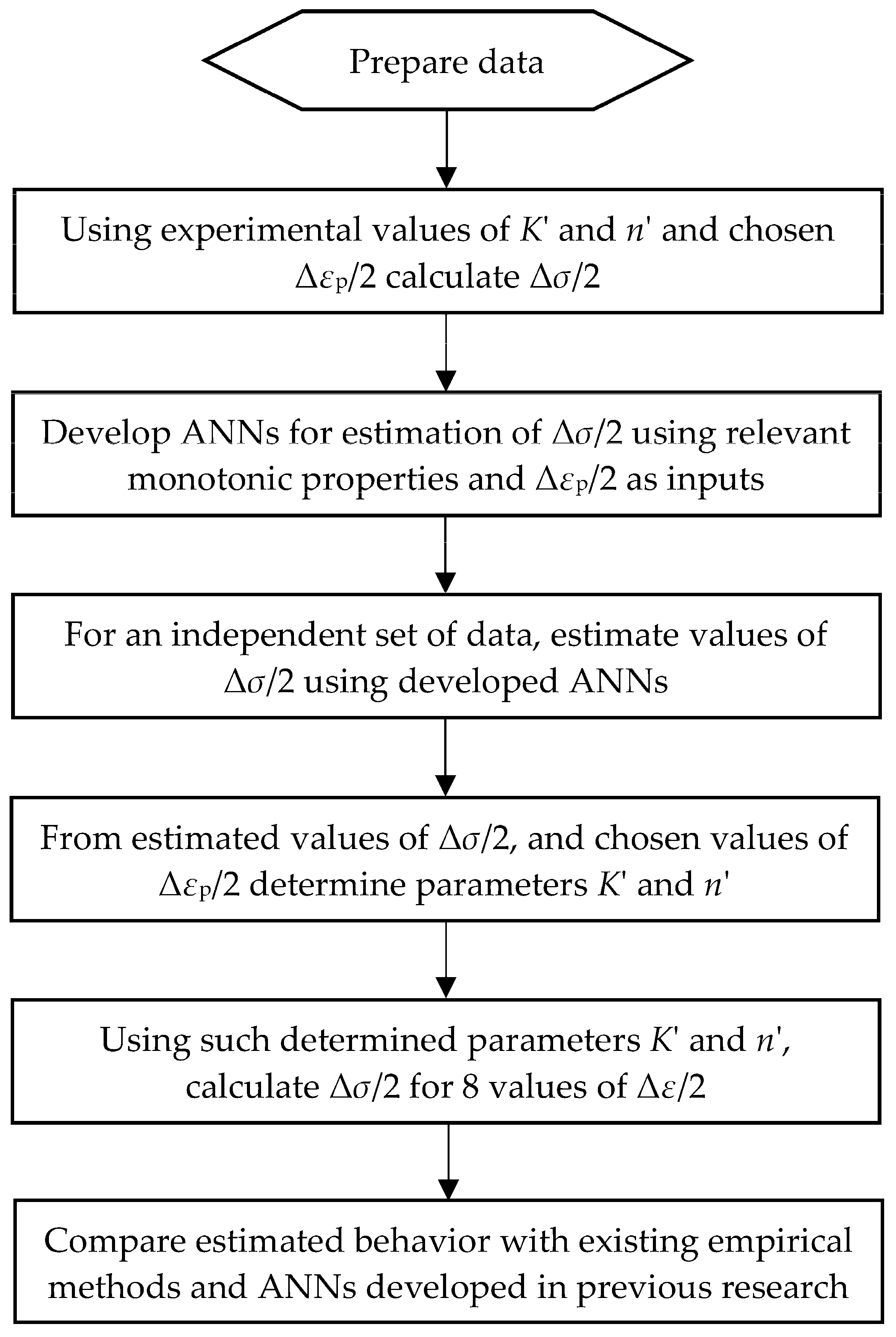
3.1. General Methodology
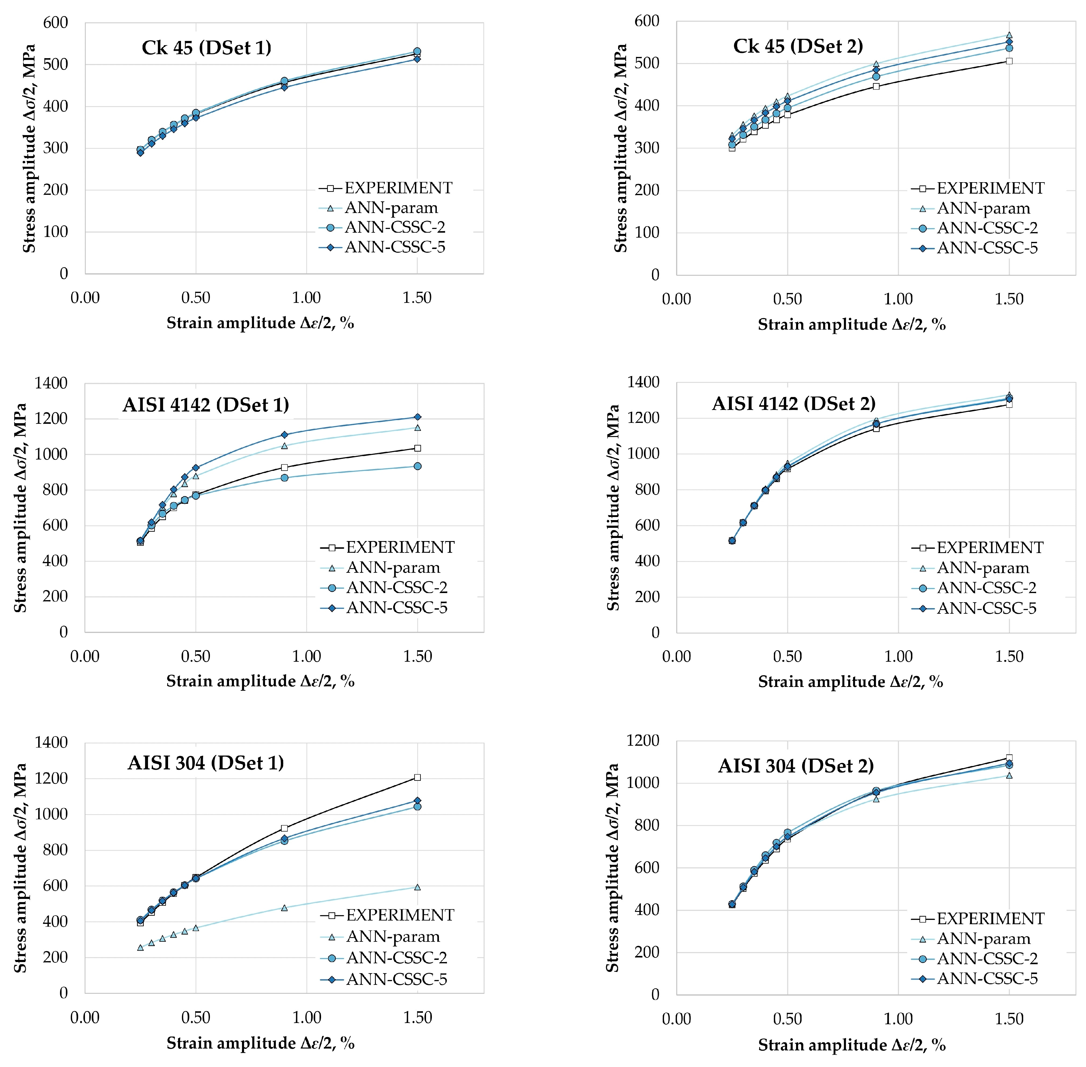
- Δσ/2 for Δεp/2 = 0.2% and 2%;
- Δσ/2 for Δεp/2 = 0.2%; 0.5%, 1%, 1.5% and 2%.
3.2. Materials Data
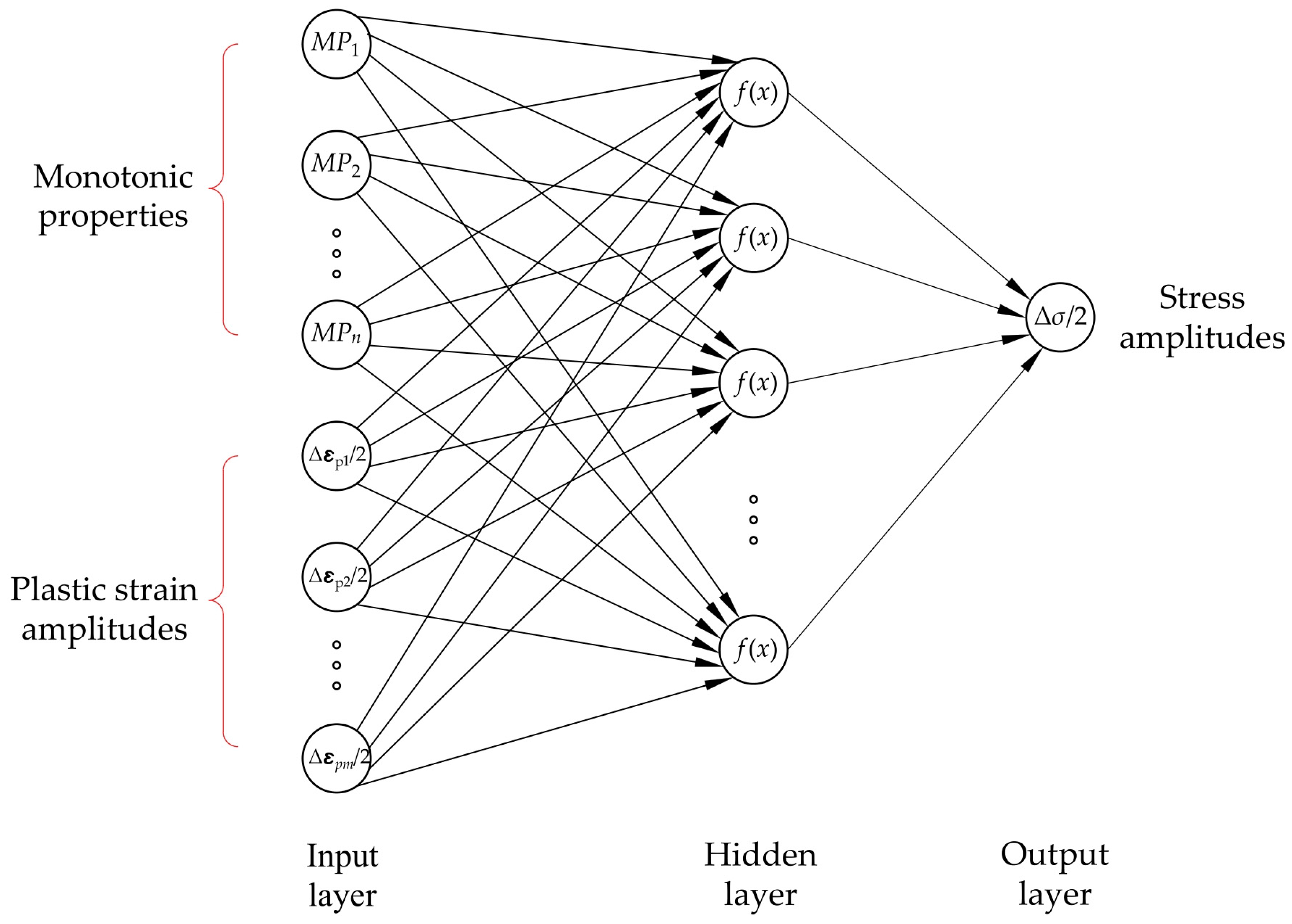
3.3. ANNs for Estimation of Cyclic Stress–Strain Behavior
4. Results
5. Performance Evaluation of ANNs and Comparison to Existing Approaches
6. Discussion and Conclusions
Author Contributions
Funding
Institutional Review Board Statement
Informed Consent Statement
Data Availability Statement
Acknowledgments
Conflicts of Interest
References
- Ramberg, W.; Osgood, W.R. Description of Stress-Strain Curves by Three Parameters; Technical Note No. 902; National Aeronautics and Space Administration: Washington, DC, USA, 1943.
- Zhang, Z.; Qiao, Y.; Sun, Q.; Li, C.; Li, J. Theoretical Estimation to the Cyclic Strength Coefficient and the Cyclic Strain-Hardening Exponent for Metallic Materials: Preliminary Study. J. Mater. Eng. Perform. 2009, 18, 245–254. [Google Scholar] [CrossRef]
- Basan, R.; Franulović, M.; Hanza, S.S. Estimation of Cyclic Stress-Strain Curves for Low-Alloy Steel from Hardness. Metalurgija 2010, 49, 83–86. [Google Scholar]
- Lopez, Z.; Fatemi, A. A Method of Predicting Cyclic Stress-Strain Curve from Tensile Properties for Steels. Mater. Sci. Eng. A 2012, 556, 540–550. [Google Scholar] [CrossRef]
- Li, J.; Zhang, Z.; Li, C. An Improved Method for Estimation of Ramberg-Osgood Curves of Steels from Monotonic Tensile Properties. Fatigue Fract. Eng. Mater. Struct. 2016, 39, 412–426. [Google Scholar] [CrossRef]
- Li, J.; Sun, Q.; Zhang, Z.P.; Li, C.W.; Qiao, Y.J. Theoretical Estimation to the Cyclic Yield Strength and Fatigue Limit for Alloy Steels. Mech. Res. Commun. 2009, 36, 316–321. [Google Scholar] [CrossRef]
- Zonfrillo, G. New Correlations Between Monotonic and Cyclic Properties of Metallic Materials. J. Mater. Eng. Perform. 2017, 26, 1569–1580. [Google Scholar] [CrossRef]
- Derrick, C.; Fatemi, A. Correlations of Fatigue Strength of Additively Manufactured Metals with Hardness and Defect Size. Int. J. Fatigue 2022, 162, 106920. [Google Scholar] [CrossRef]
- Marohnić, T.; Basan, R.; Franulović, M. Evaluation of Methods for Estimation of Cyclic Stress-Strain Parameters from Monotonic Properties of Steels. Metals 2017, 7, 17. [Google Scholar] [CrossRef] [Green Version]
- Kalla, D.K.; Sheikh-Ahmad, J.; Twomey, J. Artificial Neural Network Utilization in Modeling of Machining of Composites. In Proceedings of the International SAMPE Technical Conference, Fort Worth, TX, USA, 17–20 October 2011. [Google Scholar]
- Asiltürk, İ.; Çunkaş, M. Modeling and Prediction of Surface Roughness in Turning Operations Using Artificial Neural Network and Multiple Regression Method. Expert Syst. Appl. 2011, 38, 5826–5832. [Google Scholar] [CrossRef]
- Zhang, M.; Sun, C.N.; Zhang, X.; Goh, P.C.; Wei, J.; Hardacre, D.; Li, H. High Cycle Fatigue Life Prediction of Laser Additive Manufactured Stainless Steel: A Machine Learning Approach. Int. J. Fatigue 2019, 128, 105194. [Google Scholar] [CrossRef]
- Bao, H.; Wu, S.; Wu, Z.; Kang, G.; Peng, X.; Withers, P.J. A Machine-Learning Fatigue Life Prediction Approach of Additively Manufactured Metals. Eng. Fract. Mech. 2021, 242, 107508. [Google Scholar] [CrossRef]
- Jia, Y.; Fu, R.; Ling, C.; Shen, Z.; Zheng, L.; Zhong, Z.; Hong, Y. Fatigue Life Prediction Based on a Deep Learning Method for Ti-6Al-4V Fabricated by Laser Powder Bed Fusion up to Very-High-Cycle Fatigue Regime. Int. J. Fatigue 2023, 172, 107645. [Google Scholar] [CrossRef]
- Mosleh, A.O.; Kotova, E.G.; Kotov, A.D.; Gershman, I.S.; Mironov, A.E. Bearing Aluminum-Based Alloys: Microstructure, Mechanical Characterizations, and Experiment-Based Modeling Approach. Materials 2022, 15, 8394. [Google Scholar] [CrossRef] [PubMed]
- Genel, K. Application of Artificial Neural Network for Predicting Strain-Life Fatigue Properties of Steels on the Basis of Tensile Tests. Int. J. Fatigue 2004, 26, 1027–1035. [Google Scholar] [CrossRef]
- Troshchenko, V.T.; Khamaza, L.A.; Apostolyuk, V.A.; Babich, Y.N. Strain-Life Curves of Steels and Methods for Determining the Curve Parameters. Part 2. Methods Based on the Use of Artificial Neural Networks. Strength Mater. 2011, 43, 1–14. [Google Scholar] [CrossRef]
- Soyer, M.A.; Kalaycı, C.B.; Karakaş, Ö. Low-Cycle Fatigue Parameters and Fatigue Life Estimation of High-Strength Steels with Artificial Neural Networks. Fatigue Fract. Eng. Mater. Struct. 2022, 45, 3764–3785. [Google Scholar] [CrossRef]
- Ghajar, R.; Naserifar, N.; Sadati, H.; Alizadeh, K.J. A Neural Network Approach for Predicting Steel Properties Characterizing Cyclic Ramberg-Osgood Equation. Fatigue Fract. Eng. Mater. Struct. 2011, 34, 534–544. [Google Scholar] [CrossRef]
- Tomasella, A.; El Dsoki, C.; Hanselka, H.; Kaufmann, H. A Computational Estimation of Cyclic Material Properties Using Artificial Neural Networks. Procedia Eng. 2011, 10, 439–445. [Google Scholar] [CrossRef]
- Marohnić, T. Estimation of Cyclic and Fatigue Parameters of Steels Based on Their Monotonic Properties Using Artificial Neural Networks. Ph.D. Thesis, University of Rijeka, Faculty of Engineering, Rijeka, Croatia, 2017. [Google Scholar]
- Marohnić, T.; Basan, R. Estimation of Cyclic Behavior of Unalloyed, Low-Alloy and High-Alloy Steels Based on Relevant Monotonic Properties Using Artificial Neural Networks. Materwiss. Werksttech. 2018, 49, 368–380. [Google Scholar] [CrossRef]
- Gangi Setti, S.; Rao, R.N. Artificial Neural Network Approach for Prediction of Stress–Strain Curve of near β Titanium Alloy. Rare Met. 2014, 33, 249–257. [Google Scholar] [CrossRef]
- Yang, C.; Kim, Y.; Ryu, S.; Gu, G.X. Prediction of Composite Microstructure Stress-Strain Curves Using Convolutional Neural Networks. Mater. Des. 2020, 189, 108509. [Google Scholar] [CrossRef]
- Lavech du Bos, M.; Balabdaoui, F.; Heidenreich, J.N. Modeling Stress-Strain Curves with Neural Networks: A Scalable Alternative to the Return Mapping Algorithm. Comput. Mater. Sci. 2020, 178, 109629. [Google Scholar] [CrossRef]
- Basan, R.; Franulović, M.; Prebil, I.; Kunc, R. Study on Ramberg-Osgood and Chaboche Models for 42CrMo4 Steel and Some Approximations. J. Constr. Steel Res. 2017, 136, 65–74. [Google Scholar] [CrossRef]
- Marohnić, T.; Basan, R. Study of Monotonic Properties’ Relevance for Estimation of Cyclic Yield Stress and Ramberg-Osgood Parameters of Steels. J. Mater. Eng. Perform. 2016, 25, 4812–4823. [Google Scholar] [CrossRef]
- Boller, C.; Seeger, T. Materials Data for Cyclic Loading, Part A–D; Elsevier Ltd.: Amsterdam, The Netherlands, 1987. [Google Scholar]
- Park, J.-H.; Song, J.-H. Detailed Evaluation of Methods for Estimation of Fatigue Properties. Int. J. Fatigue 1995, 17, 365–373. [Google Scholar] [CrossRef]
- Basan, R. MATDAT Materials Properties Database, Version 1.0. Available online: http://www.matdat.com/ (accessed on 15 January 2016).
- Baumel, A.; Seeger, T. Materials Data for Cyclic Loading—Supplement 1; Elsevier Ltd.: Amsterdam, The Netherlands, 1990. [Google Scholar]
- AISI Bar Steel Fatigue Database. Available online: http://barsteelfatigue.autosteel.org/ (accessed on 15 March 2016).
- Fatemi, A.; Zeng, Z.; Plaseied, A. Fatigue Behavior and Life Predictions of Notched Specimens Made of QT and Forged Microalloyed Steels. Int. J. Fatigue 2004, 26, 663–672. [Google Scholar] [CrossRef]
- Jen, Y.-M.; Wang, W.-W. Crack Initiation Life Prediction for Solid Cylinders with Transverse Circular Holes under In-Phase and out-of-Phase Multiaxial Loading. Int. J. Fatigue 2005, 27, 527–539. [Google Scholar] [CrossRef]
- Jones, D.; Kurath, P. Cyclic Fatigue Damage Characteristics Observed for Simple Loadings Extended to Multiaxial Life Prediction (NASA Contractor Report 182126); University of Illinois: Urbana, IL, USA, 1988. [Google Scholar]
- Koh, S.K.; Stephens, R.I. Mean Stress Effects on Low Cycle Fatigue for a High Strength Steel. Fatigue Fract. Eng. Mater. Struct. 1991, 14, 413–428. [Google Scholar] [CrossRef]
- Landgraf, R.W. Cyclic Deformation and Fatigue Behavior of Hardened Steels (T.&A.M. Report No. 320); University of Illinois: Urbana, IL, USA, 1968. [Google Scholar]
- Roessle, M.L.; Fatemi, A. Strain-Controlled Fatigue Properties of Steels and Some Simple Approximations. Int. J. Fatigue 2000, 22, 495–511. [Google Scholar] [CrossRef]
- Smith, R.W.; Hirschberg, M.H.; Manson, S.S. Fatigue Behavior of Materials under Strain Cycling in Low and Intermediate Life Range (Technical Note D-1574); Lewis Research Center: Cleveland, OH, USA, 1963. [Google Scholar]
- Subramanya Sarma, V.; Padmanabhan, K.A. Low Cycle Fatigue Behaviour of a Medium Carbon Microalloyed Steel. Int. J. Fatigue 1997, 19, 135–140. [Google Scholar] [CrossRef]
- Technical Report on Low Cycle Fatigue Properties Ferrous and Non-Ferrous of Materials (J1099_197502); SAE International: Warrendale, PA, USA, 1975.
- Wang, Y.-Y.; Yao, W.-X. A Multiaxial Fatigue Criterion for Various Metallic Materials under Proportional and Nonproportional Loading. Int. J. Fatigue 2006, 28, 401–408. [Google Scholar] [CrossRef]
- The MathWorks Inc. MATLAB, Version: 9.13.0 (R2022b); The MathWorks Inc.: Natick, MA, USA, 2022. [Google Scholar]
- Smokvina Hanza, S.; Marohnić, T.; Iljkić, D.; Basan, R. Artificial Neural Networks-Based Prediction of Hardness of Low-Alloy Steels Using Specific Jominy Distance. Metals 2021, 11, 714. [Google Scholar] [CrossRef]
- Asteris, P.G.; Mokos, V.G. Concrete Compressive Strength Using Artificial Neural Networks. Neural Comput. Appl. 2020, 32, 11807–11826. [Google Scholar] [CrossRef]
- Armaghani, D.J.; Asteris, P.G. A Comparative Study of ANN and ANFIS Models for the Prediction of Cement-Based Mortar Materials Compressive Strength. Neural Comput. Appl. 2021, 33, 4501–4532. [Google Scholar] [CrossRef]


| Steel Group | Independent Variables (Monotonic Properties) | |||||||||
|---|---|---|---|---|---|---|---|---|---|---|
| Modulus of Elasticity E | Yield Stress Re or Rp0.2 | Ultimate Strength Rm | Ultimate Strength to Yield Stress Ratio Rm/Re | Ultimate Strength to Modulus of Elasticity Ratio Rm/E | Reduction of are at Fracture RA | Strength Coefficient K | Strain Hardening exponent n | True Fracture Stress σf | Modulus of Elasticity E | |
| UA | + | + | + | + | UA | |||||
| LA | + | + | + | LA | ||||||
| HA | + | + | + | + | N/A | N/A | N/A | HA | ||
| Steel Subgroup | Value | Monotonic Properties | Cyclic Parameters | ||||||||||||
|---|---|---|---|---|---|---|---|---|---|---|---|---|---|---|---|
| HB (HB) | E (MPa) | Re or Rp0.2 (MPa) | Rm (MPa) | Rm/Re (-) | Rm/E (10−3) | RA (%) | K (MPa) | n (-) | σf (MPa) | εf (-) | R’p0.2 (MPa) | K′ (MPa) | n′ (-) | ||
| UA | Min | 130 | 190,000 | 207 | 359 | 1.159 | 1.710 | 0 | 330 | 0.015 | 653 | 0.000 | 239 | 813 | 0.085 |
| Max | 385 | 217,510 | 760 | 1018 | 1.848 | 4.966 | 74 | 1606 | 0.285 | 1784 | 1.204 | 722 | 2407 | 0.254 | |
| Mean | 216 | 206,594 | 474 | 665 | 1.437 | 3.222 | 59 | 1033 | 0.165 | 1228 | 0.864 | 408 | 1263 | 0.184 | |
| Alloying element content range (wt%): C 0.02–0.50; Si 0.02–0.55; Mn 0.03–1.50; P 0.01–0.05; S 0.01–0.05; Cr 0.02–0.19; Mo 0.00–0.01; Ni 0.01–0.13; Cu 0.01–0.21; Al 0.04–0.07; N 0.00–0.01 | |||||||||||||||
| LA | Min | 23 | 187,500 | 330 | 540 | 1.038 | 2.700 | 3 | 717 | 0.007 | 926 | 0.026 | 322 | 894 | 0.067 |
| Max | 357 | 221,000 | 1927 | 2016 | 1.855 | 9.739 | 76 | 2586 | 0.236 | 2230 | 1.450 | 1341 | 3328 | 0.225 | |
| Mean | 225 | 201,658 | 857 | 987 | 1.184 | 4.910 | 56 | 1298 | 0.084 | 1522 | 0.847 | 647 | 1419 | 0.125 | |
| Alloying element content range (wt%): C 0.04–1.02; Si 0.06–0.68; Mn 0.01–1.43; P 0.01–0.04; S 0.00–0.06; Cr 0.03–1.89; Mo 0.01–1.13; Ni 0.02–1.90; Cu 0.01–0.57; Al 0.00–0.17; Co 0.00–0.21; Ti 0.00–0.04; V 0.06–0.24; Nb 0.00–0.03 | |||||||||||||||
| HA | Min | 35 | 172,625 | 177 | 516 | 1.231 | 2.457 | 46 | 349 | 0.062 | 1360 | 1.010 | 197 | 987 | 0.093 |
| Max | 337 | 210,000 | 795 | 1158 | 3.670 | 5.521 | 83 | 1416 | 0.362 | 2407 | 1.715 | 882 | 8384 | 0.469 | |
| Mean | 168 | 205,811 | 331 | 685 | 2.428 | 3.342 | 71 | 791 | 0.157 | 1837 | 1.402 | 377 | 2567 | 0.305 | |
| Alloying element content range (wt%): C 0.02–0.25; Si 0.27–1.50; Mn 0.41–2.00; P 0.02–0.04; S 0.00–0.02; Cr 11.40–25.00; Mo 0.02–2.62; Ni 0.21–24.65; Cu 0.06–0.31; Al 0.00–0.26; Co 0.11–0.22; Ti 0.00–2.50; W 0.00–0.99; V 0.00–0.28; N 0.05–0.25 | |||||||||||||||
| Parameter | Value |
|---|---|
| Training algorithm | Levenberg–Marquadt (with early stopping) |
| Normalization | minmax in the range from −1 to 1 |
| Number of hidden layers | 1 |
| Number of neurons per hidden layer | 1 to H by step 1 UA: 2 data points H = 13; 5 data points H = 33 LA: 2 data points H = 18; 5 data points H = 46 HA: 2 data points H = 6; 5 data points H = 16 |
| Control random number generation | rng(‘default’), Mersenne Twister generator with seed 0 |
| Number of trainings per architecture | 10 |
| Training goal | 0.0001σtarget2 |
| Epochs | 1000 (if MSE not met) |
| Cost function | MSE |
| Transfer function | tansig; purelin |
| Number of k-folds | 10 |
| Division of data into k-fold | random permutation |
| σtarget2 variance of the target variable | |
| MSE mean square error | |
| Tansig: hyperbolic tangent sigmoid transfer function | |
| Purelin: linear transfer function | |
| Steel Group | Data Points Used for Estimation | H | RMSEmean,test | rtest |
|---|---|---|---|---|
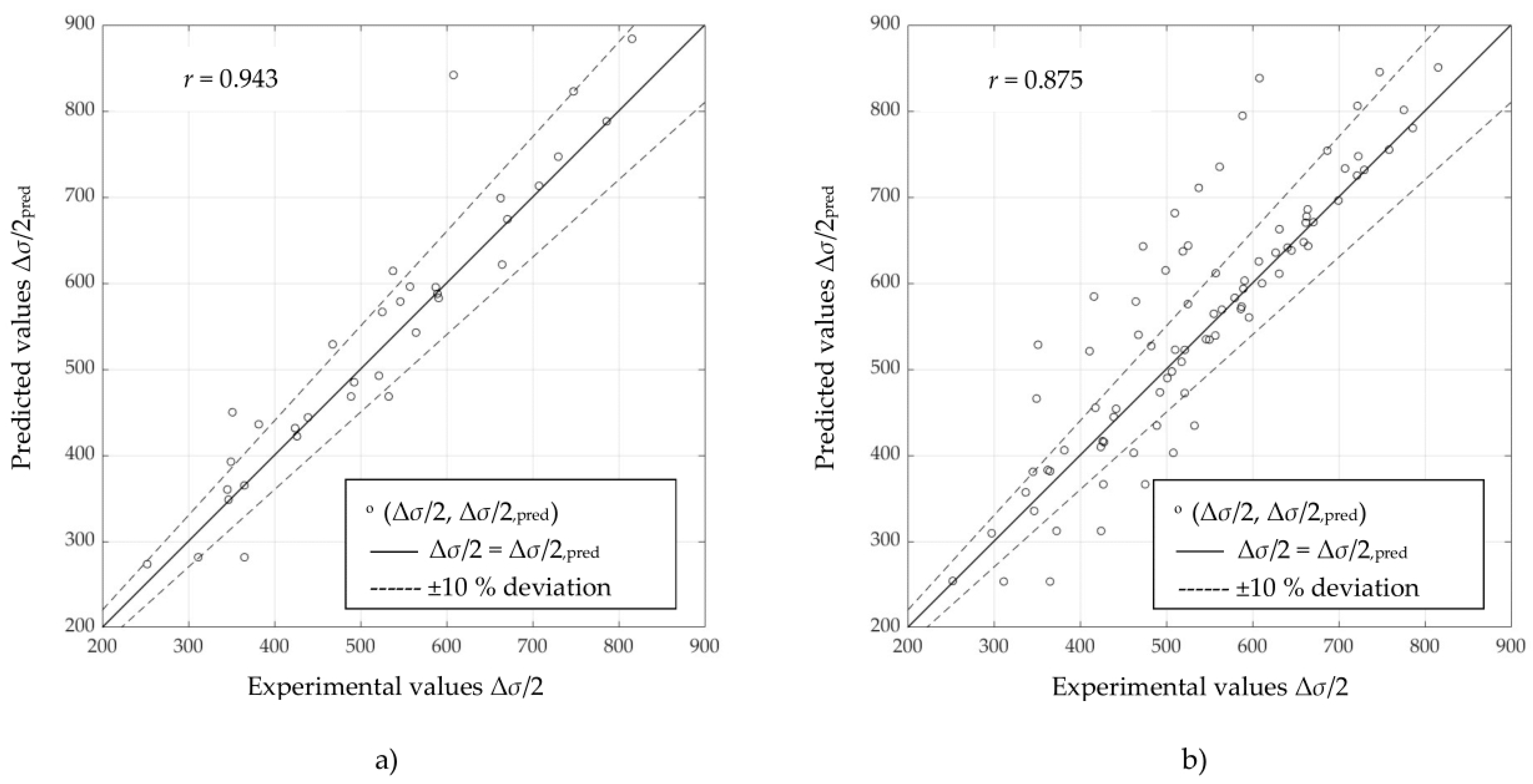
| UA | 2 | 12 | 57 | 0.943 |
| 5 | 17 | 75 | 0.875 | |
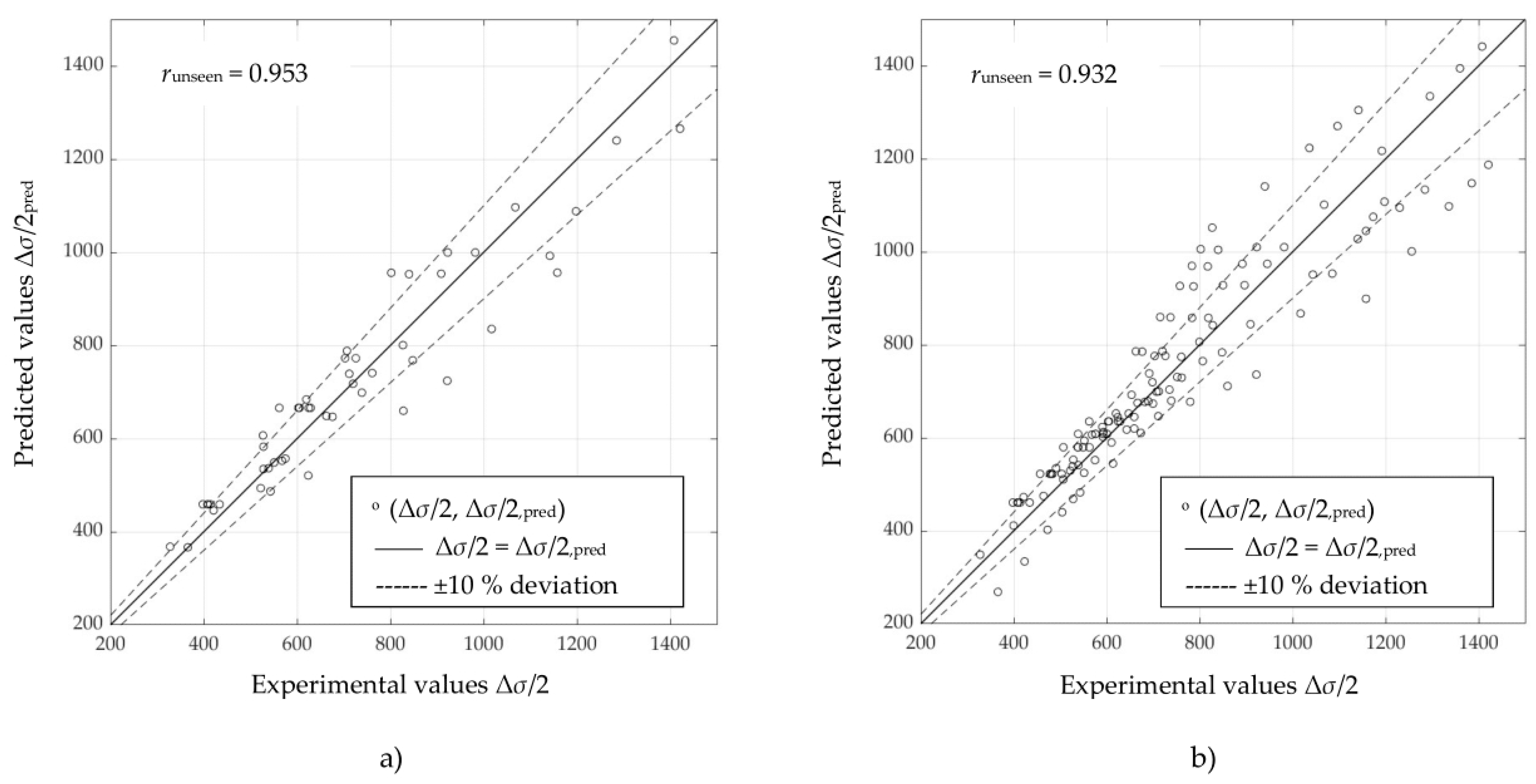
| LA | 2 | 13 | 82 | 0.953 |
| 5 | 19 | 93 | 0.932 | |
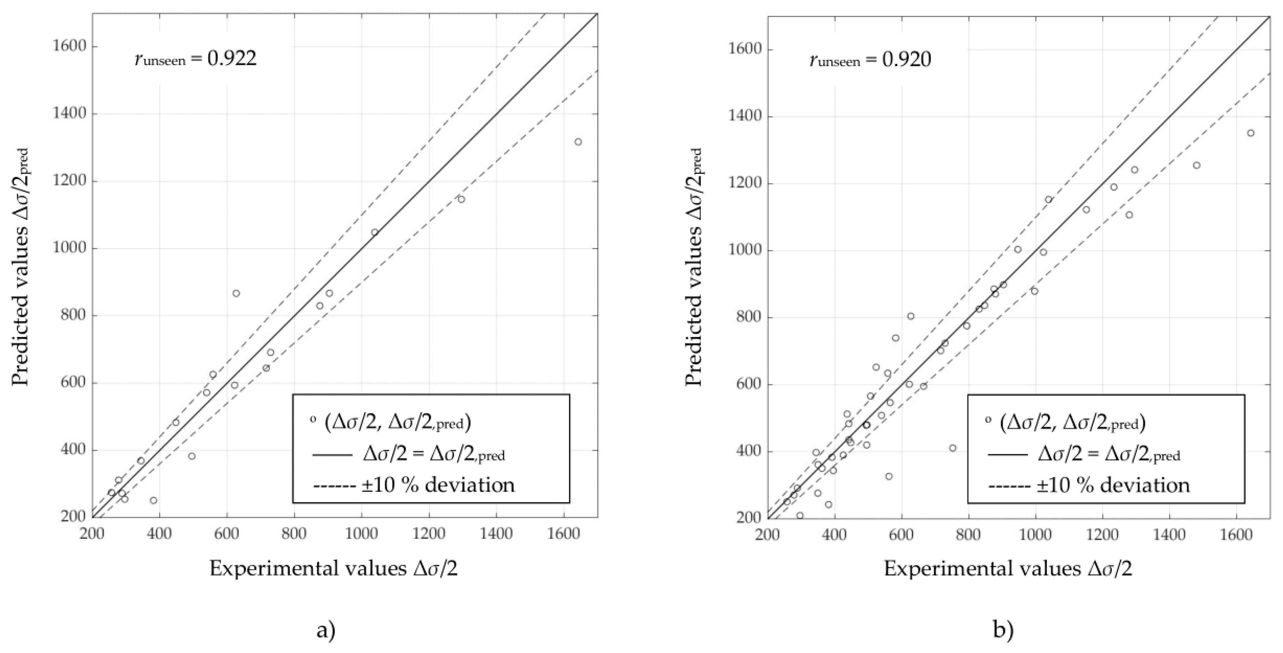
| HA | 2 | 5 | 151 | 0.922 |
| 5 | 10 | 137 | 0.920 |
| Steel Group | Method/Approach | MAPE | RMSE |
|---|---|---|---|
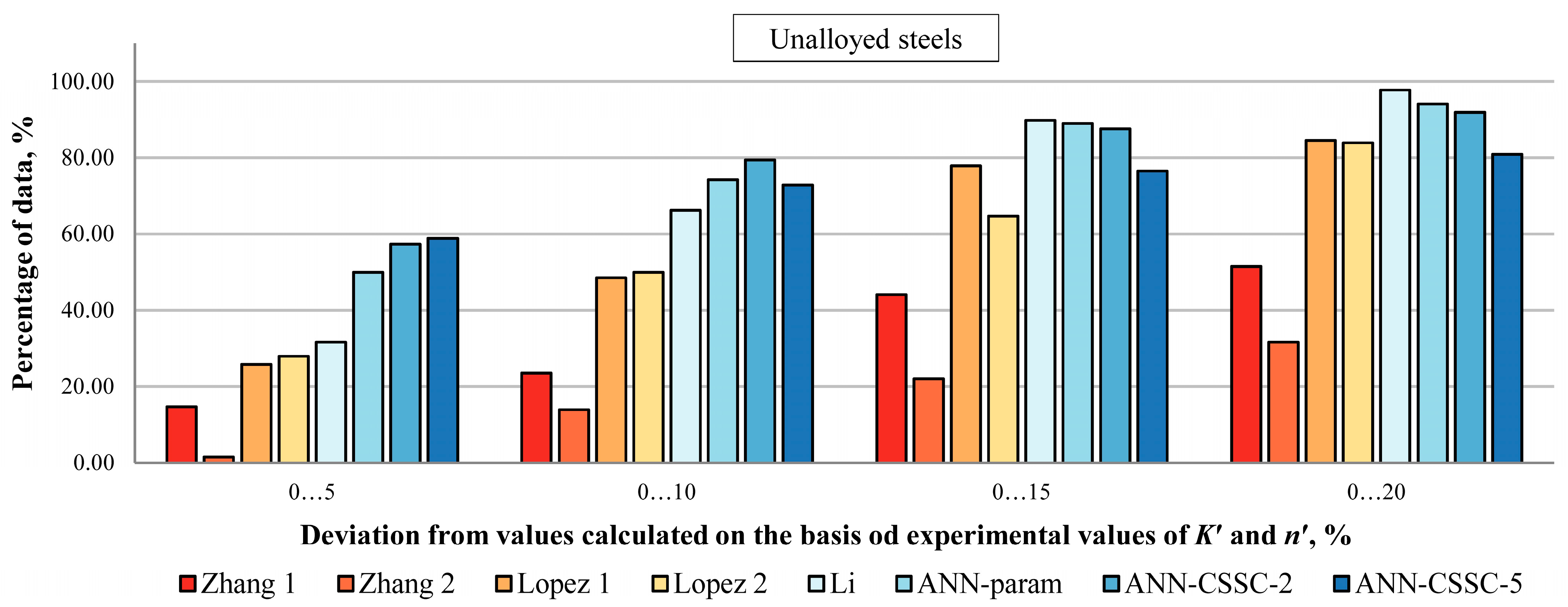
| UA | Zhang 1 [2] | 26.13 | 182.78 |
| Zhang 1 [2] | 34.08 | 192.79 | |
| Lopez 1 [4] | 12.92 | 68.28 | |
| Lopez 1 [4] | 11.82 | 59.02 | |
| Li [5] | 8.17 | 44.07 | |
| ANN-param [22] | 6.83 | 39.81 | |
| ANN-CSSC-2 | 6.19 | 38.18 | |
| ANN-CSSC-5 | 9.47 | 57.61 | |
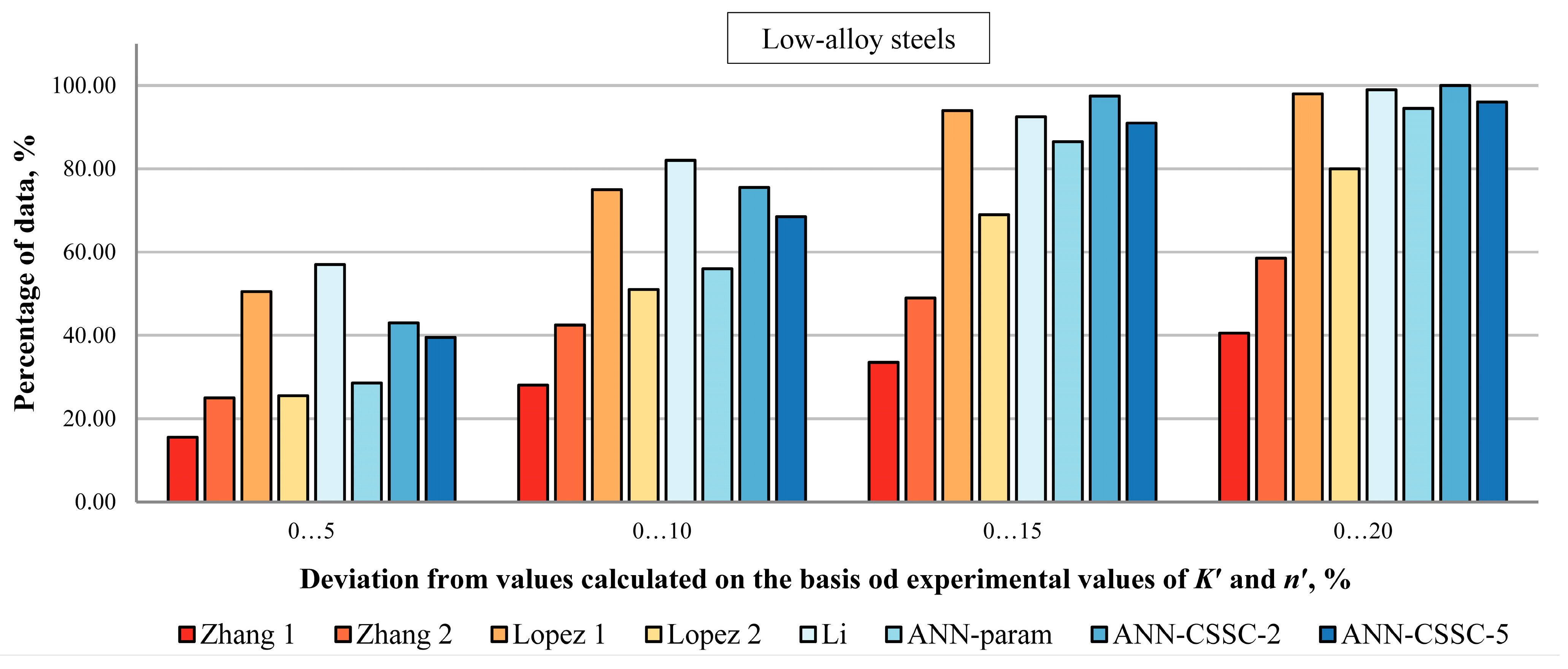
| LA | Zhang 1 [2] | 37.96 | 270.33 |
| Zhang 1 [2] | 19.79 | 157.46 | |
| Lopez 1 [4] | 6.38 | 56.28 | |
| Lopez 1 [4] | 11.54 | 78.23 | |
| Li [5] | 5.88 | 54.06 | |
| ANN-param [22] | 9.06 | 61.70 | |
| ANN-CSSC-2 | 6.48 | 48.92 | |
| ANN-CSSC-5 | 7.70 | 59.82 | |
| HA | Zhang 1 [2] | 82.64 | 332.49 |
| Zhang 1 [2] | 28.05 | 175.82 | |
| Lopez 1 [4] | 20.11 | 173.56 | |
| Lopez 1 [4] | 22.19 | 183.31 | |
| Li [5] | 20.91 | 129.90 | |
| ANN-param [22] | 14.96 | 136.43 | |
| ANN-CSSC-2 | 9.62 | 68.52 | |
| ANN-CSSC-5 | 8.98 | 68.05 |
Disclaimer/Publisher’s Note: The statements, opinions and data contained in all publications are solely those of the individual author(s) and contributor(s) and not of MDPI and/or the editor(s). MDPI and/or the editor(s) disclaim responsibility for any injury to people or property resulting from any ideas, methods, instructions or products referred to in the content. |
© 2023 by the authors. Licensee MDPI, Basel, Switzerland. This article is an open access article distributed under the terms and conditions of the Creative Commons Attribution (CC BY) license (https://creativecommons.org/licenses/by/4.0/).
Share and Cite
Marohnić, T.; Basan, R.; Marković, E. Estimation of Cyclic Stress–Strain Curves of Steels Based on Monotonic Properties Using Artificial Neural Networks. Materials 2023, 16, 5010. https://doi.org/10.3390/ma16145010
Marohnić T, Basan R, Marković E. Estimation of Cyclic Stress–Strain Curves of Steels Based on Monotonic Properties Using Artificial Neural Networks. Materials. 2023; 16(14):5010. https://doi.org/10.3390/ma16145010
Chicago/Turabian StyleMarohnić, Tea, Robert Basan, and Ela Marković. 2023. "Estimation of Cyclic Stress–Strain Curves of Steels Based on Monotonic Properties Using Artificial Neural Networks" Materials 16, no. 14: 5010. https://doi.org/10.3390/ma16145010