1. Introduction
As part of compliance with the regulations governing good practices related to the use of energy in electrical systems, power quality is an aspect of great importance that is used when determining the characteristics of electrical energy. In recent decades, there has been increasing interest in the study and development of techniques aimed at improving power quality, motivated by the increasingly stringent quality requirements derived from new grid codes and standards [
1]. It should be noted that non-compliance with power-quality regulations can result in a penalty and even force a generator to be disconnected from the utility grid.
As shown in [
2], alterations in the sinusoidal voltage and current waveforms may occur in the production, transport, and distribution processes, as well as in energy use by certain types of loads. Therefore, they are unavoidable. However, only in recent years have they become a cause for concern. In the utility grid, among the different disturbances that can be found, one of the most predominant is harmonic distortion, which is mainly due to the existence of non-linear loads, which are defined by a pure non-sinusoidal demand current and, therefore, by a distorted wave [
3,
4,
5]. This harmonic pollution can introduce current distortions in the utility grid [
6].
Grid tie (grid-connected) inverters have played an extremely interesting role in the incorporation of renewable energy sources (RES) into the utility grid. Power electronics converters (PEC) and control interfaces are critical for the power conditioning required for the integration of RES-based distributed generation (DG). Nevertheless, important challenges are associated with the increasing number of PE interfaces in the electrical utility: stability under weak grid conditions, limited short-circuit current, and nonlinear dynamics [
7,
8]. The nonlinear nature of switching devices and their high-frequency operation are important contributors to the increased presence of harmonics in utility grids with high penetration of RES and PEC [
9]; thus, the study of harmonic compensation techniques as auxiliary services of PEC interfaces is an important issue for enabling large-scale integration of RES and DG. Due to the above factors, various studies focused on the use of techniques to improve power quality in relation to current harmonic distortion have been presented in the scientific literature [
10,
11,
12,
13,
14,
15,
16,
17,
18,
19].
Microgrids are defined as a collection of DG and loads (critical and non-critical) with the capability for either islanded or grid-tied operation [
20]. As discussed in [
21], the presence of current harmonics may present important challenges in the operation of microgrid systems. These harmonics can affect internal PEC measurements, causing voltage distortion at the point of common coupling (PCC) and, in case of large harmonic presence, lead to the activation of the PEC’s internal protection. From this perspective, the study of auxiliary services related to harmonic compensation inside of microgrids is of importance.
As harmonics reduce electrical power quality, this paper will focus on the mitigation of harmonics in inverters used in PV generators in a microgrid configuration connected to the utility grid. The methodology will be based on the creation of a model in MATLAB/SIMULINK R2022a of a PV generator belonging to a microgrid affected by grid disturbances such as harmonic distortion, fundamental frequency variation and voltage unbalance. A study of the grid currents with and without a HC strategy will be conducted on the PV generator of the microgrid using MATLAB’s Fast Fourier Transform (FFT) analyzer [
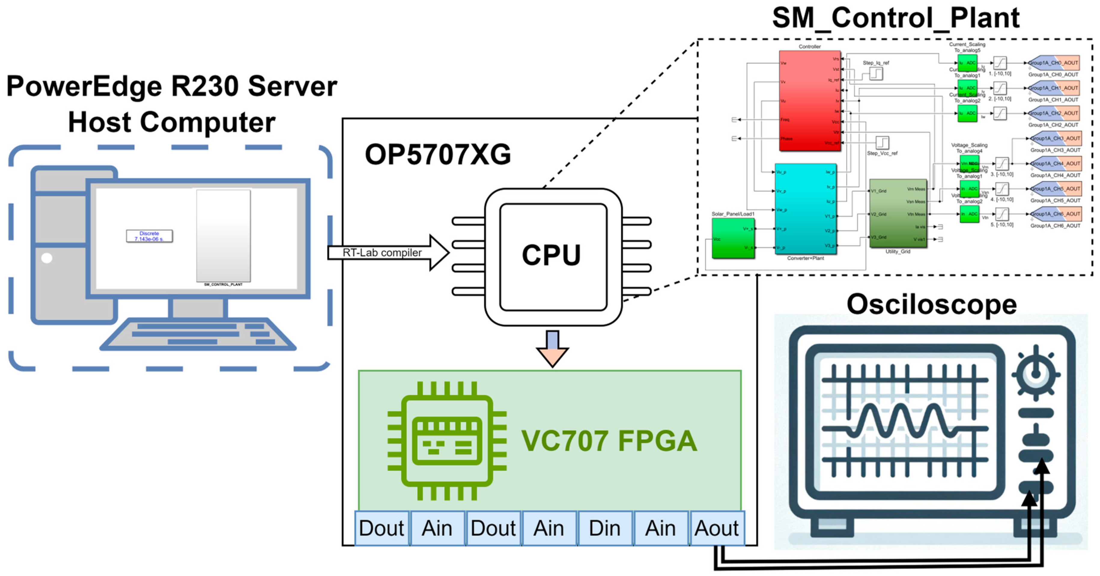
22]. The FFT represents a calculation algorithm that provides the content of the different pure sine waves that make up the deformed wave. A final validation of the HC structures is carried out through real-time simulations using an OP5707XG simulator from OPAL-RT [
23]. As shown in [
24], these types of validation are of relevance for the implementation of advanced control techniques focused on harmonics mitigation. Nevertheless, hardware constraints limit the number of harmonic compensation structures that can be implemented. Thus, it is of importance to test how this new generation of digital simulators may enable the simulation of more complex harmonic compensation structures.
The contributions of this research can be summarized in three main points: firstly, a bibliographic analysis of different strategies used for current harmonic compensation in grid-connected inverters; secondly, a detailed explanation of the modeling of a HC structure using MATLAB/SIMULINK; and finally, the real-time validation of a harmonic compensation structure up to the 17th harmonic, taking advantage of the new simulation capacities presented by the OP5707XG simulator from Opal RT. This approach allows the demonstration of the improvement in energy quality realized by using harmonic compensation techniques in inverters of photovoltaic generators connected to utility grid affected by harmonic pollution and other grid disturbances.
Different methodologies used for harmonic compensation and improved power quality in PV generators in microgrid configurations are discussed in
Section 2. In
Section 3, a case study of a microgrid is explained. The methodology used in this paper is shown in
Section 4. To study the harmonic behavior of the case studies, various simulations using MATLAB/SIMULINK are described in
Section 5. Several real-time tests performed using a digital simulator are described in
Section 6. The discussion of the results obtained is shown in
Section 7. Finally, some conclusions are presented in
Section 8.
2. Review of Grid Tie Inverter Control Techniques for Harmonic Compensation
Below, some works from the scientific literature aimed at improving quality, in terms of harmonic mitigation, in microgrids and distributed generation systems are discussed. These works were selected by searching for keywords such as “harmonic compensation”, “microgrids”, and “distributed generation”. The journals where they were published and their impact were also taken into consideration.
In the review presented in [
10], the authors comment on the versatility of operation offered by PEC-based microgrids (MG), which can be used in either an islanded or a grid-tie operation. This versatility creates an array of opportunities for providing auxiliary services to the electrical utility with the goal of improving power quality indicators. Typically, the control structure of microgrids has been separated into three hierarchical levels. The primary level oversees internal voltage/frequency regulation; the secondary level monitors and compensate for deviations in the primary-level control variables; and finally, the tertiary control level ensures correct energy management under grid-tie or grid-forming operation. Nevertheless, harmonic presence due to nonlinear loads, switching, and resonance is an important problem for the implementation of hierarchical control. As mentioned by the authors, numerous investigations have been carried out on harmonic compensation using the PEC of the MG systems. These studies have focused on one of the following objectives: harmonic mitigation at the common connection point (PCC), harmonic cancellation in local loads, and mitigation of line current harmonics. The first step in the harmonic compensation process is detection, wherein spectral-analysis methods like the discrete Fourier transform (DFT) and the sliding DFT (SDFT) have been applied. In the first compensation strategies, authors elaborated on primary-level compensation methods, among them modified droop control (MDC), adaptive virtual impedance (VIA), and proportional-resonance regulator (PR). Harmonic compensation at the secondary level can be separated in two principal approaches: centralized and distributed. In both, the main objective is the online monitoring of harmonic presence for each MG with the purpose of adjusting the harmonic compensation at the individual level. Finally, compensation at the tertiary level focuses on the optimization process, in which optimal set points are selected to minimize the harmonic presence of each MG. In their conclusion, the authors comment on the directions future research must take in order to develop inverter-based harmonic compensation, highlighting the importance of improved and more powerful control methods based on predictive control or artificial intelligence approaches. Additionally, it is important to note that the harmonic compensation structures reviewed by the authors were directed to the 11th harmonic and bellow, making a case for the evaluation of the design of higher-order harmonic compensation structures, as proposed by this work.
Classical proportional resonant methods for harmonic compensation are shown in [
11]. The presented frequency-adaptive architecture can be tuned by using the information provided by the harmonic detection strategy. This detection procedure is carried out using a modified second-order generalized integrator (SOGI) together with a synchronous reference frame phase-locked loop (SRF-PLL). The authors study the bandwidth of the SOGI and the capacity of the SRF-PLL to compensate for harmonics outside its central frequency, adding an adaptive parameter for the detection of the harmonic with the higher amplitude without losing stability. The validation is done by means of harmonic injection-induced variation. In their results, the authors comment on the adaptability of the proposed strategy, which is capable of reducing the harmonic with the greatest amplitude and of adding more SRF-PLL stages for further harmonic compensation. Nevertheless, the considerations for the evaluation of the system account for only the 3rd and the 5th harmonics.
In [
12], a strategy for harmonic compensation using grid-tie converters and considering capacity limitations is presented. The authors note that previous works do not consider constraints related to the capacity of the inverter; that is, the rated apparent power of the inverter should not exceed the active and the apparent power rating of the inverter during the harmonic compensation process. To achieve the above aim, the proposed control strategy calculates the maximum allowable current for harmonic compensation. The harmonics are detected using the d-q current reference frame, where the current waveforms are low-pass filtered and subtracted to determine the harmonic content. A regulation factor is calculated for the maximum allowable harmonic compensation current. Two harmonic compensation strategies are compared: quasi-proportional resonant (QPR) and vector resonant (VR) controller; both strategies provide better robustness compared to traditional proportional resonant (PR) control. These controllers are coupled with a traditional proportional-integral (PI) control for the internal DC loops in the d-q reference frame for the operation of the inverter. In their results, the authors show the harmonic suppression of the PI + QPR strategy under capacity limitation, validating their proposed strategy. A point is made concerning the inter-harmonic coupling, which affects the compensation strategy in both controllers. Nevertheless, the best results are obtained with the PI + VR strategy due to its better performance in harmonic tracking, with a reduction of THD from 7.69% to 3.78%. This paper concludes by noting the good performance of the proposed strategies and the need for future research regarding the inter-harmonic coupling effect to improve performance with regard to harmonic suppression. This inter-harmonic coupling effect recognized by the authors is an important motivator in studies of the design of higher-order HC structures like the one proposed in this work.
The development of resonant converters for harmonic compensation is also studied in [
13]; the authors comment on the computational burden imposed by multiple resonant controllers (MRSCs) if compensation is required for various harmonic frequencies. Furthermore, there are stability issues related to RSC in cases of utility frequency deviation. Such issues require the adaptive online tuning of these types of controllers. The authors proposed a novel downsampling method to reduce the computational burden imposed by multiple MRSCs that uses a multi-rate resonant controller implementation. The developed methodology creates a multirate RSC combining the 6th, 12th, and 18th harmonics and uses power-hardware-in-the-loop (PHIL) simulations for validation. The results show that the computational burden is reduced by a factor of two with the proposed strategy and that the obtained THD is below 6% for each of the studied cases. The article concludes by recommending this type of strategy for the deployment of embedded inverter control systems and the reduction of total system costs. This work is a good reference regarding enhanced performance in higher-order HC compensation structures; in this paper, this type of strategy will be incremented to include the 3rd, 5th, 7th, 11th, 13th, 15th, and 17th harmonics, taking advantage of the increased hardware performance of the latest generation of digital simulators.
The deployment of advanced optimization techniques to improve the harmonic characteristics of PEC is presented in [
14]. A modified grey wolf optimization algorithm (MGWO) is proposed to solve the nonlinear problematic of selective harmonic elimination pulse width modulation (SHE-PWM) and offers better harmonic suppression performance compared to other modulation strategies. The improved exploration and exploitation capabilities of the proposed MGWO algorithm offer advantages over other types of optimization strategies such as particle swarm optimization (PSO), traditional grey wolf optimization (GWO), or genetic algorithms (GA). The proposed MGWO introduces a chaotic variable to enhance the exploration and exploitation capabilities of traditional GWO. In the methodology, nonlinear switching equations that account for harmonics up to the 13th harmonic are presented. They are used with the purpose of solving the system of equations to reduce the presence of harmonics. Various tests are conducted under different modulation indices to validate the proposed strategy. The proposed MGWO could produce a THD of 5.54% with a modulation index of 0.6 and a THD of 6.03% with a modulation index of 1.1, offering a lower THD when compared to the GWO solution. Validations were conducted in simulated and physical environments; in their conclusions, the authors comment on the rapidity with which the MGWO was able to obtain the solutions required for the harmonic reduction strategies.
As several PEC interfaces may operate in parallel under MG islanded operation, the evaluation of harmonic suppression at the PCC is of interest. The authors of [
15] studied the implementation of coordinated control strategies for harmonic compensation involving several DG agents. For this purpose, an adaptive virtual impedance controller (VIC) is used to compensate for THD at the PCC. The VIC is a modification of the classical droop controller, where a virtual impedance is applied to enhance reactive power sharing. This approach can be extended to provide harmonic compensation at the PCC, as demonstrated by the authors using a negative virtual impedance value. Additionally, the authors formulated a strategy for the regulation of PCC voltage and harmonic levels that involved dividing the virtual impedance into two components. A microgrid central controller (MGCC) manages the operation of each individual VIC and provides the necessary reference points to achieve the desired harmonic compensation level based on each measurement of the PCC harmonic distortion. Robustness against communication delays was tested for the centralized control system, and it was found that a communication delay of 10 ms can be tolerated. The results show a harmonic reduction with the proposed strategy, where the initial 7.55% THD was reduced to 2.76%. The simulation was conducted using four DG units, and a physical implementation of the system was constructed using three inverters. In the physical implementation, the initial harmonic presence was 6.20%, and after the activation of the VIC strategy, a reduction to 3.07% was obtained. In their conclusions, the authors comment on the viability of the proposed strategy, which is due to its simple implementation.
As can be seen from [
15], the dependency on a centralized controller is an important limitation in the implementation of multiagent harmonic compensation strategies.
In [
16], a distributed event-triggered approach for the multiagent compensation of harmonics by means of PEC is described. Stability conditions for the proposed control system were studied using Lyapunov formulations. In this approach, events are triggered by the deviation error from the desired total harmonic value. After this step, each internal harmonic compensation network of the agents is adjusted by the consensus rule proposed by the authors. The stability of the consensus criterium is tested, and experimental results are produced. The testing involves a nonlinear load producing 3.5% THD, which is reduced to levels below 1%. Various cases are studied, with changes in the information shared between each agent and maintenance of the correct harmonic compensation. The authors conclude by discussing the robustness of the proposed strategy and the possibility of discretizing event monitoring to reduce the communication burden.
Due to increasing use of hybrid AC/DC MG, the authors of [
17] present a harmonic compensation strategy for the DC bus in a hybrid MG based on the use of GA. In the case of DC sub grids inside a MG, the even-numbered harmonics are presented. This paper focuses on mitigating the 2nd harmonic by means of introducing a compensation current that acts like a virtual impedance. The GA algorithm calculates the set point for this current, executing an online evaluation of its fitting function. Results from both simulated and physical implementations show a reduction in voltage ripple on the DC bus, from 16.2 V to less than 2.5 V in both scenarios. The presented conclusions comment on the viability of using the GA algorithm for online optimization; furthermore, the proposed methodology was validated by the obtained results.
In the research presented in [
25], the authors use a harmonic compensation strategy based on the use of parallel resonant filters. Each resonant filter corresponds to the harmonic that will be compensated for within the control current loop used in the inverter of a grid-connected photovoltaic generator. This harmonic compensation strategy allows for frequency-adaptive harmonic compensation, since the frequency estimated by the synchronization algorithm is relayed to the harmonic compensation block. This ability of this harmonic compensation technique to adapt to frequency variations makes it attractive for use in settings in which photovoltaic generators are connected to a weak electrical grid susceptible to electrical disturbances. The biggest drawback of this technique is that a high PWM switching frequency is necessary to compensate for harmonics exceeding the 13th order.
The work presented in [
26] introduces a new procedure aimed at optimally designing harmonic control and compensation strategies for three-phase inverters with grid support in AC microgrids. The strategy is based on a three-level cascade control developed in the stationary system ab, using PI and PR regulators. The authors note that the proposed strategy can reduce the THD and the individual harmonic distortion of the voltages in the microgrid. In the presence of nonlinear loads, the voltage THD could be decreased to 0.19%. The design of the optimized harmonic compensation strategy and the inverter controller utilized an optimization algorithm called H-HHOPSO. This optimization algorithm was developed through a hybridization between a particle swarm optimization algorithm and a Harris Hawks optimization algorithm. The validation of the proposed strategy was carried out using models created in MATLAB/SIMULINK. The design of the controller and the optimized HC strategy was divided into two stages. The purpose of the first stage was the calculation and selection of the parameters corresponding to the voltage and current control of the inverter through PR regulators and the harmonic compensation strategy. In the second stage, the coefficients of the droop control controllers, the secondary control level and the synchronization control were designed.
The proposed strategy was compared with other harmonic compensation techniques when non-linear loads were connected, and the THD of voltage in the microgrid was reduced from 5.23% to 4.18% when a traditional control based on a PI regulator was used. When the H-HHOPSO strategy presented by the authors was used, the voltage THD was reduced to 0.16%. It should be noted that other types of grid disturbances such as voltage unbalance and voltage flickers were not considered in the study. Furthermore, it should be noted that the evaluation of the proposed technique was validated through simulations.
Table 1 summarizes the harmonic compensation strategies described above, classifying them by the technique used to detect harmonics, the compensation method, the harmonic reduction, the limitations of the studies carried out, and finally, the validation method. As can be seen from the limitations of the reviewed works, the higher-order HC structure designed in this paper is significant because it enables the study of compensating a broader range of harmonics in the proposed MG real-time test case.
5. MATLAB/SIMULINK Simulations
In this section, a MATLAB/SIMULINK model of a 3.68 kWp single-stage PV generator in a microgrid schema is presented. The power subsystem includes a PELab-6PH-SiC-8A-2LC25-4.7uF-16CH-INT Dual 3-phase Voltage Source Inverter 8 A Leg, 800 V DC-Link Max from Taraz Technologies. This system uses semiconductors [
46] and is configured to operate at a PWM switching frequency of 35 kHz. It includes six 2.5 mH inductors and two EMC filters, each with a capacity of 4.7 uF. The parameters for this inverter are detailed in this work, as can be seen in
Table 4, which outlines the parameters of the power subsystem.
To guarantee accurate detection of the phase angle of the grid voltages, as well as precise estimation of the grid frequency to be relayed to the control subsystem, an MSOGI-FLL is used as a synchronization algorithm [
29]. In various works, this algorithm has been implemented due to its effectiveness in handling disturbances in the three-phase utility grid [
25,
45,
47]. In
Table 5, the parameters of the control subsystem are summarized.
Table 4.
Parameters of the power subsystem.
Table 4.
Parameters of the power subsystem.
| Parameters | Value |
|---|
| Link capacitor (Clink) | 15,000 μF |
| Switching frequency (fsw) | 35 kHz |
| Line inductance (L) | 2.5 mH |
| AC system (ugrst) | 120 V(rms) phase-to-neutral
Frequency: 60 Hz and 65 Hz |
| Transformer resistance (RT) | 0.0231 Ω |
| Transformer inductance (LT) | 2400 µH |
Table 5.
Parameters of the control subsystem.
Table 5.
Parameters of the control subsystem.
| Parameters | Value |
|---|
| Proportional constant of the PR regulator (KPαβ) | 0.15 |
| Integral constant of the PR regulator (KIαβ) | 10 |
| Resonant angular frequency of the PR regulator (ωo′) | 377/408.408 rad/s |
| Cut-off frequency of the PR regulator (ωc) | 1 rad/s |
| Proportional constant of the DC voltage regulator (KPVDC) | 0.2813 |
| Integral constant of the DC voltage regulator (KIVDC) | 8.81 |
| Phase margin of the inner current loop (PMI) | 83° |
| Phase margin of the outer voltage loop (PMV) | 63.5° |
| Sample time of the power subsystem (TS) | 1.0417 μs |
| Sample time of the control subsystem (Treg) | 33.3 μs |
| Time constant () | |
| Full-scale range of the ADC (FSR) | 1 |
| Gain of the current transducer GTI | 1 |
| Inverter gain (KINV) | |
The dynamics of the current control loop can be evaluated using a Bode plot. Using the parameters given in
Table 4 and
Table 5, the open-loop Bode diagram shown in
Figure 5 was created for the fundamental grid frequency and for the 5th, 7th, 11th, 13th, and 17th harmonics. There is a phase margin of 83 degrees for a frequency of 60 Hz and for a frequency increase of 5 Hz (65 Hz). The above finding suggests that the internal current control will remain stable during variations in the grid frequency. This characteristic is useful in a microgrid affected by harmonic pollution and simultaneous frequency variations.
To investigate the harmonic compensation method selected for this work, a SIMULINK model of a microgrid has been developed, taking as reference some of the elements shown in
Figure 1. The SIMULINK model shown in
Figure 6 includes a comprehensive 11 kWp grid-connected photovoltaic (PV) system comprising three PV generators, each rated at 3.68 kW, and real weather station data. Additionally, the system includes a resistive programmable load, one power-management subsystem, and a variety of different measurement scopes throughout the system. The color of each block represents the group to which it belongs: yellow represents weather data, red represents power systems, blue represents control subsystems, purple represents grid loads, and white represents measurement points. In the section below, a detailed explanation of each block is provided.
The weather station data block includes an extensive 6-month real-world database that stores irradiance and temperature measurements taken from a Vantage Pro 2 integrated sensor suite, then outputs the information for a preselected day found in that time frame. Afterward, weather data is directly supplied to a PV array SIMULINK block featuring an array of eight series-connected 460 W Q.PEAK DUO XL-G9.3 solar panels.
The MPPT or non-MPPT algorithm controls the quantity of power produced by the PV array by providing a reference voltage point to the decoupled axis control block for the inverter to follow. It works in two operational modes based on the implemented algorithm: either it extracts the maximum available power thought a MPPT algorithm or it limits power by a constant or flexible power factor (FP) provided from the reference power port. Systems employing what are typically known as flexible power point tracker (FPPT) algorithms allow for more complete synergy with the electrical grid. They actively control the total generated power to match that expressly required by the power at a given moment. Aside from the reference voltage out port, this block also features an output port for a maximum power tracker (MPT) algorithm that calculates the maximum available power of the PV generator.
Decoupled axis control, as the names implies, contains a decoupled axis control strategy for the inverter. In this strategy, real and reactive power are extracted from the time-domain components of the three-phase electrical grid system and operated independently of one another to obtain the target specified by the MPPT or FPPT algorithm.
The DC/AC converter (VSI) encompasses all the power elements of a single-stage PV generator. It includes a PELab-6PH three-phase voltage source inverter, one DC-link 1500 uF capacitor, an LC filter, and a 208Δ/208Y three-phase transformer.
The PV array power management subsystem focuses on appropriate independent power distribution among all the PV generators. Based on the absolute error formula, this block proportionally divides the required grid power among all three generators, such that, regardless of the maximum available power of each PV plant, the load is always fairly distributed across all generators.
The programmable load consists of five constant time-triggered three-phase resistive loads in a Y connection, which can be instructed to connect or disconnect from the power grid at any given moment.
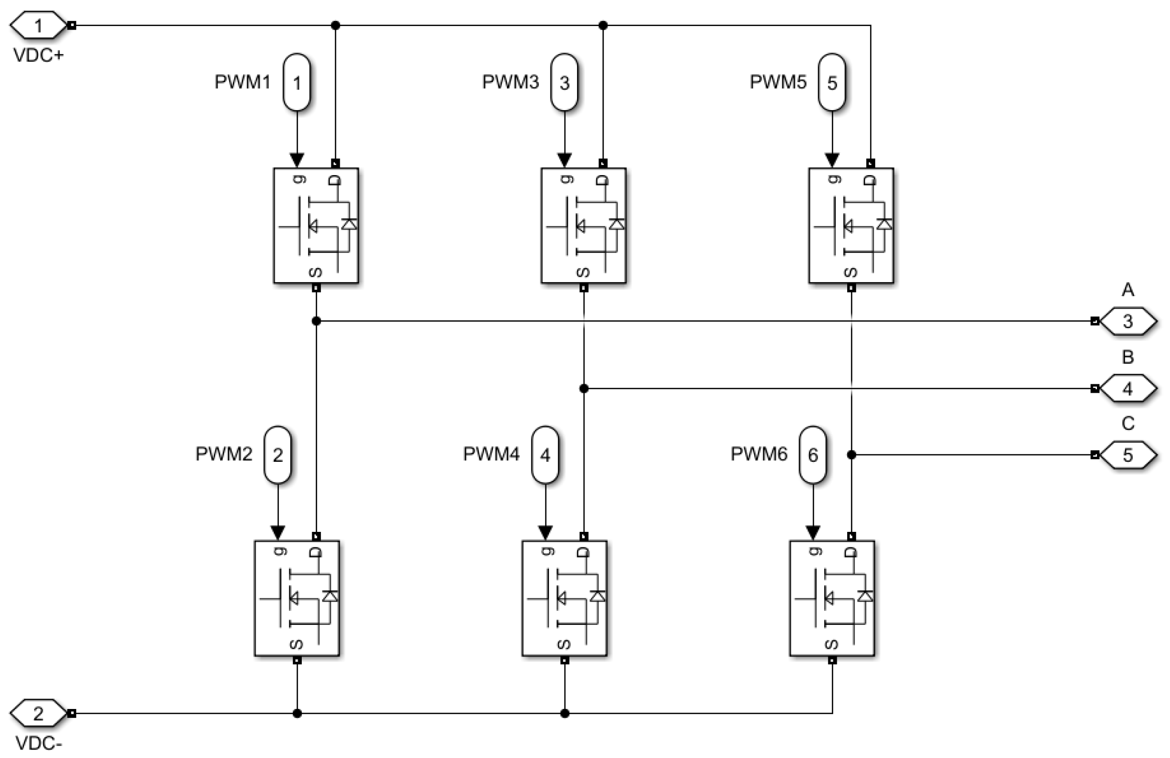
Figure 7 shows a three-phase inverter model corresponding to one of the photovoltaic generators of the microgrid depicted in
Figure 6. This model was developed using parameters corresponding to the technical specifications of a PELab-6PH-SiC-8A-2LC25-4.7uF-16CH-INT Dual 3-phase VSI 8 A Leg, 800 V DC-Link Max from Taraz Technologies [
46]. The PWM switching frequency is set at 35 kHz (FPWM = 35 kHz).
A MATLAB/SIMULINK model of the LC inverter-filter assembly with inductance and capacitance values of 2.5 mH and 4.7 uF, respectively, is shown in
Figure 8.
Figure 9 shows the implementation in MATLAB/SIMULINK of the control used in the PV inverter. At the top, in yellow, is the block with the MSOGI-FLL algorithm. The PI regulator of the external voltage loop is shown in green. In red, the PR regulators for the internal loop are shown.
Figure 10 shows the implementation in MATLAB/SIMULINK of the HC structure corresponding to Equation (7). Note at the top, in red, the proportional constant
of the PR regulator. Placed in cascade are the resonant filters corresponding to the fundamental frequency and each of the harmonics to be compensated for. The fundamental frequency is sent to each of the resonant filters with the purpose of achieving control capable of adapting to variations in the grid frequency.
Simulation Results
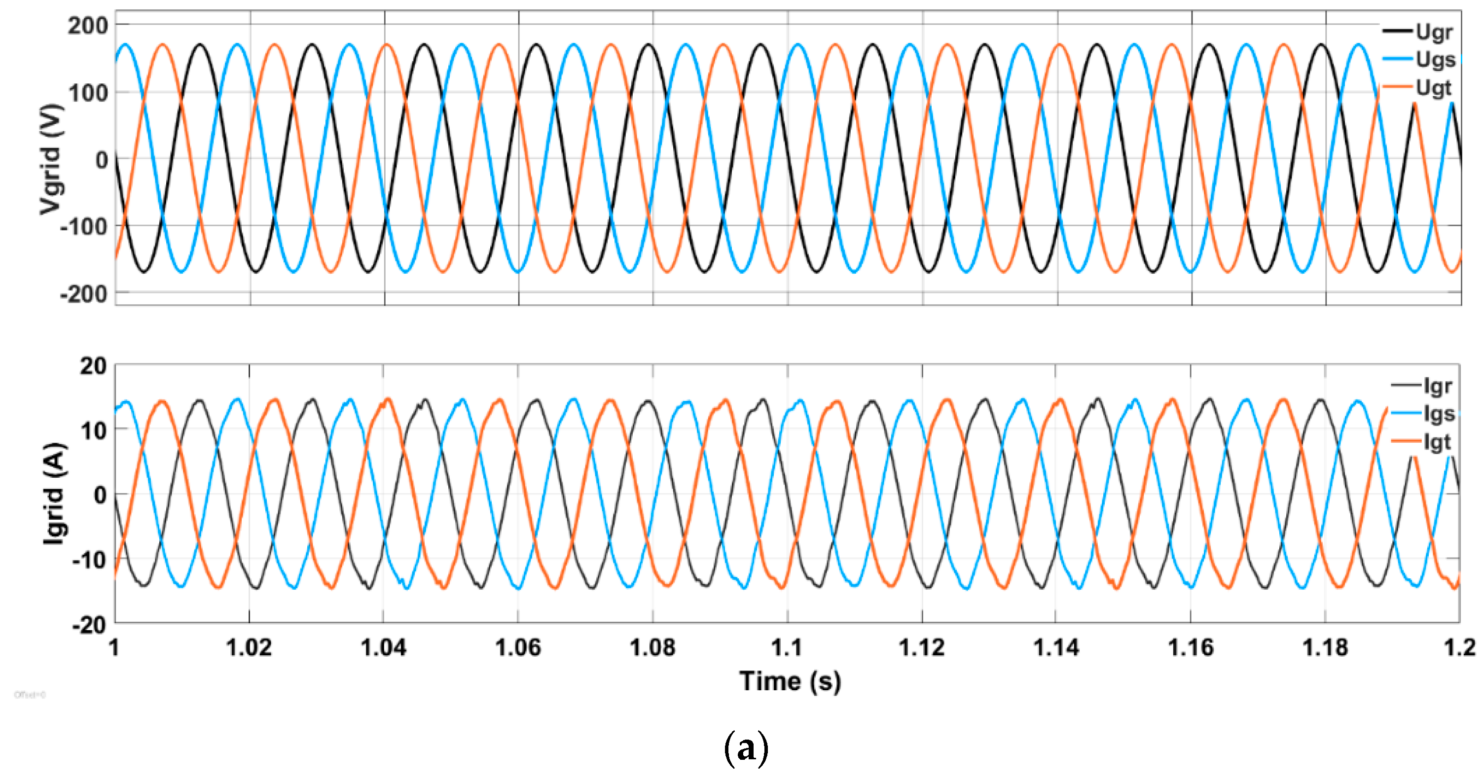
The upper part of
Figure 11a shows the evolution over time of the voltages of the utility grid. No harmonics have been introduced into the grid voltages to evaluate the grid currents of the PV generator, which has a power of 3.68 kW. The bottom part of
Figure 11a shows the evolution over time of the grid currents from the simulation when no voltage harmonics are introduced. The grid currents exhibit a low amount of harmonics distortion, leading to a total harmonic distortion (THD) of 1.14% at phase 1 (see
Figure 11b). The Fast Fourier Transform (FFT) analysis tool from MATLAB/SIMULINK [
22] was used to determine the THD of the acurrent (THD
I).
In the simulation shown below, a 15% harmonic contamination of the 5th, 7th, 11th, 13th, and 17th harmonics in the grid voltages is applied to the grid voltages (see upper part of
Figure 12a), resulting in a TDH of voltage (THD
V) of 33.54%, as can be observed in
Figure 12b. Note that the bottom part of
Figure 12a shows the distortion in the grid currents caused by the effect of voltage harmonics, leading to a current THD of 7.27% at phase 1, as can be seen in
Figure 12c. In this scenario, no harmonic compensation strategy is used in the control of the inverter, leading to non-compliance with the harmonic distortion limits established by the IEEE Std. 519-2022 standard [
1].
In the upper part of
Figure 13a, the grid voltages are illustrated with a THD
V of 33.55%. In the bottom part of
Figure 13a, the grid currents are shown with a low amount of harmonic distortion, obtaining a THD
I of 1.69% (see
Figure 13b). The above results indicate the importance of using harmonic compensation strategies to improve the quality of electrical energy in microgrids.
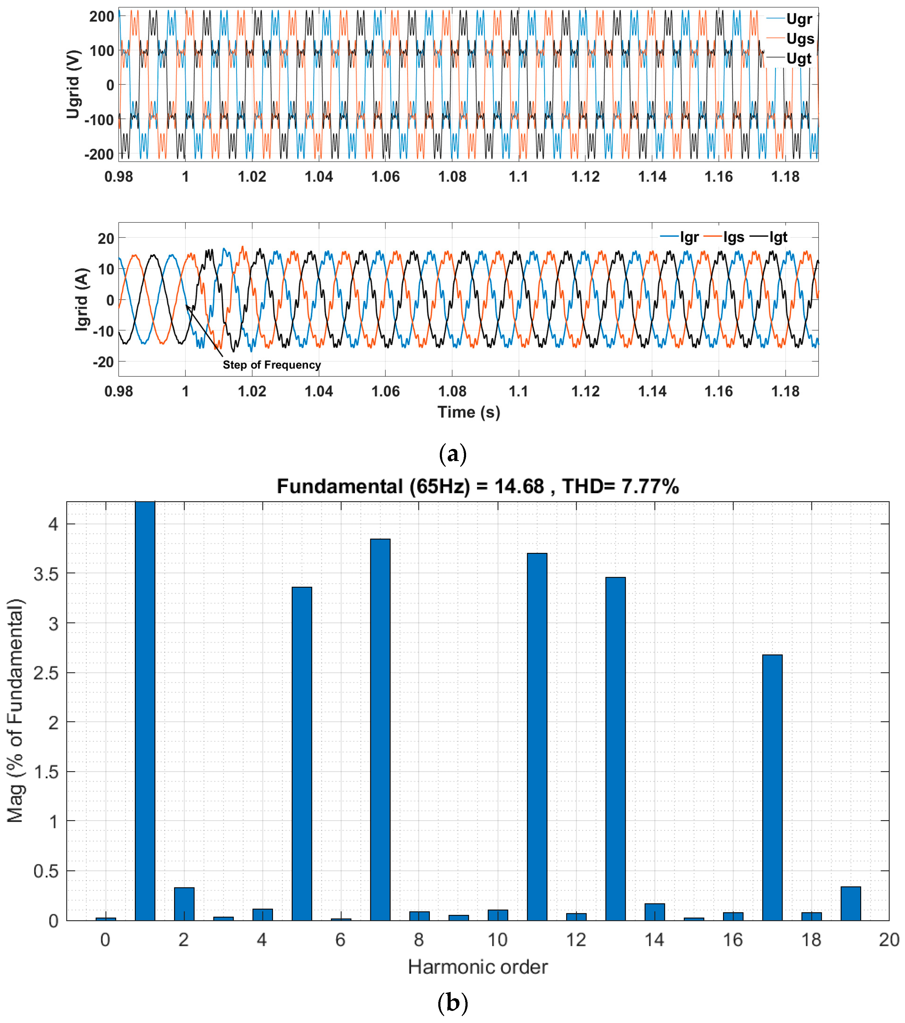
In the simulations shown below, a THDV of 33.54% is applied. In addition, a frequency step from 60 Hz to 65 Hz is applied to evaluate the harmonic behavior of the PV generator under conditions of both harmonic distortion and variations in the grid frequency.
Figure 14 shows the distorted grid voltages during a frequency step from 60 Hz to 65 Hz. As shown in the bottom part of
Figure 14a, before the frequency step, the grid currents had a low amount of harmonic distortion due to the use of a harmonic compensation strategy. However, following the frequency shift, the grid currents become distorted, reaching a THD
I of 7.77%, as can be observed in
Figure 14b. In
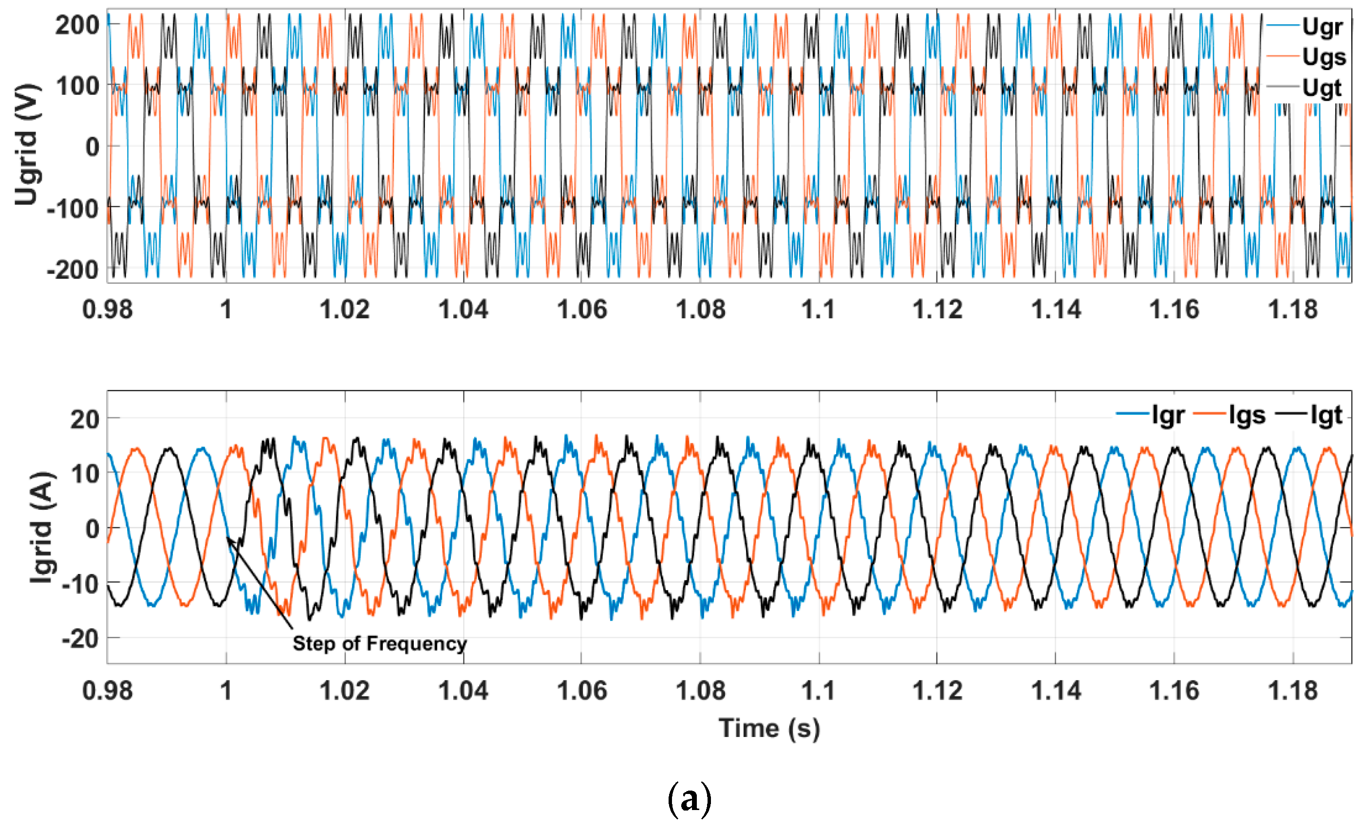
Figure 15, the grid conditions of
Figure 14 have been replicated; however, harmonic compensation technique with frequency adaptation of Equation (9) has been used, resulting in a THD
I of 3.10% at phase 1. The above observations suggest that in microgrids with frequency variations, employing a frequency-adaptive HC strategy is advisable.
In the fourth and final scenario, the ability of the PV generator to compensate for harmonics under various grid disturbances is tested by adding harmonic distortion (THD
V = 33.54%), frequency variation (step from 60 Hz to 65 Hz), and voltage unbalance (
,
,
= 169.8 V, 127.14 V, and 84.9 V, respectively).
Figure 16 shows the three-phase utility grid affected by the three types of disturbances: voltage unbalance, frequency variation, and harmonic pollution (see top of
Figure 16a). Despite the presence of the grid disturbances, the use of an adaptive-frequency HC strategy resulted in a THD
I of 1.26% at phase 1 (see
Figure 16b). Due to the voltage unbalance, an increase in the grid currents can be noted.
7. Discussion
A summary of the THDI obtained under the different scenarios and using harmonic compensation technique configurations with resonant filters is shown. In the first scenario, the THDI of phase 1 of the grid current was measured when there were no disturbances in the utility grid. Only PR regulators were used to control the inverter currents, resulting in a THD of 1.14% on the grid current at phase 1. In the second scenario, a 15% harmonic pollution was applied to the 5th, 7th, 11th, 13th, and 17th harmonics in the three-phase voltages of the utility grid were applied, leading to a TDH of voltage (THDV) of 33.54%. First, the current harmonic distortion was determined at phase 1 when only PR regulators were employed for control; second, the THD was determined when the resonant compensation strategy was used, resulting in THDI = 7.27% and THDI = 1.69%, respectively.
A THD
V of 33.54% in the utility voltages combined with a variation in the grid frequency constitute the third scenario used in the study of the harmonics of the PV generator. In the first simulation for this scenario, the harmonic compensation strategy was used without frequency feedback from the mains, resulting in a THD
I of 7.77%, a value fails to comply with international standards on harmonic distortion [
1]. In the second simulation of this scenario, the grid frequency estimated by the synchronization algorithm was incorporated into the PR + HC strategy, resulting in a THD
I of 3.10% in phase 1.
In the fourth scenario, the three-phase utility grid is affected by three types of disturbances: voltage unbalance, frequency variation, and harmonic pollution. As can be seen in
Table 6, despite the presence of grid disturbances, the use of a harmonic compensation strategy resulted in a THD
I of 1.26% at phase 1, ensuring compliance with the established harmonic limits.
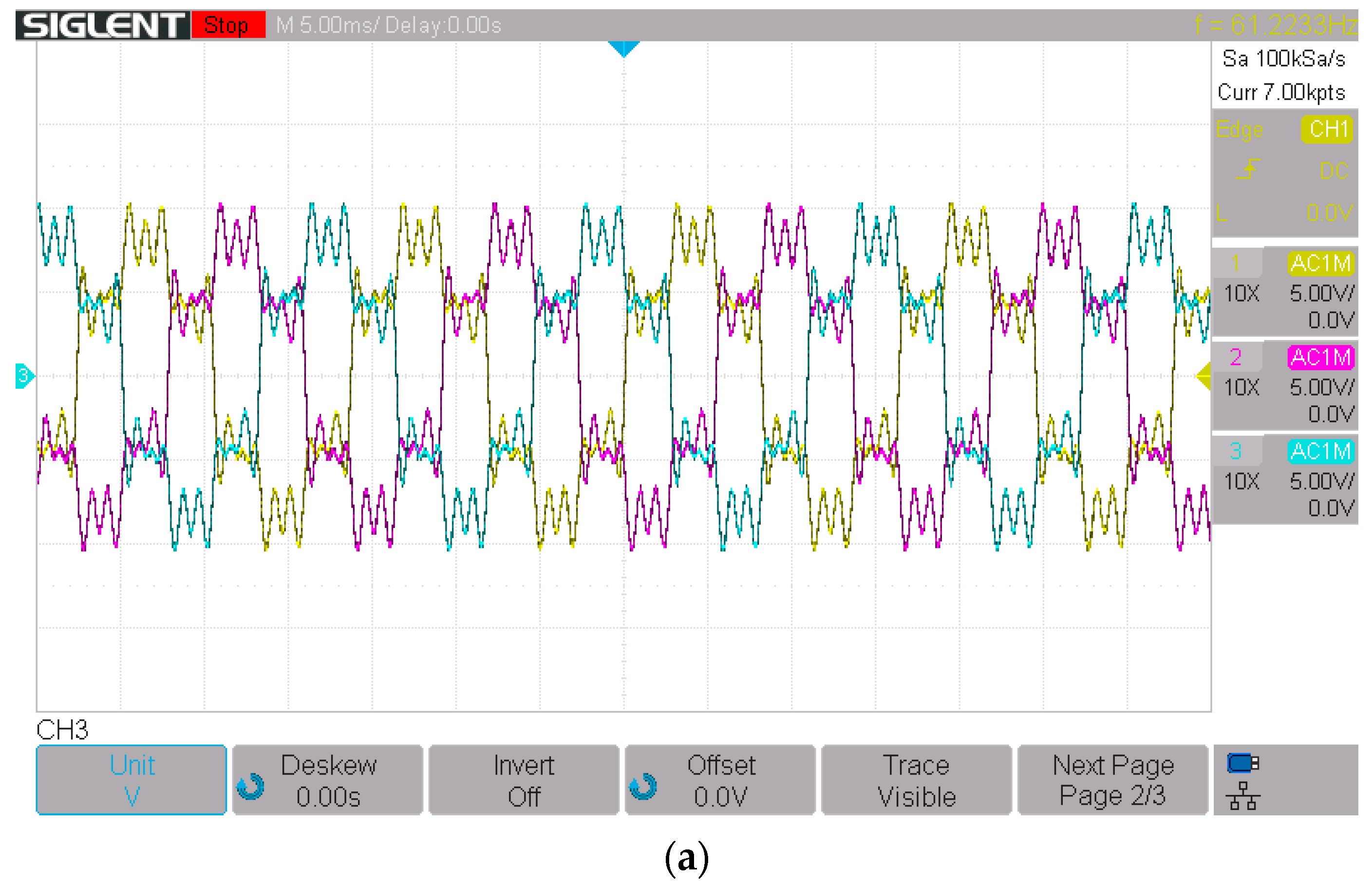
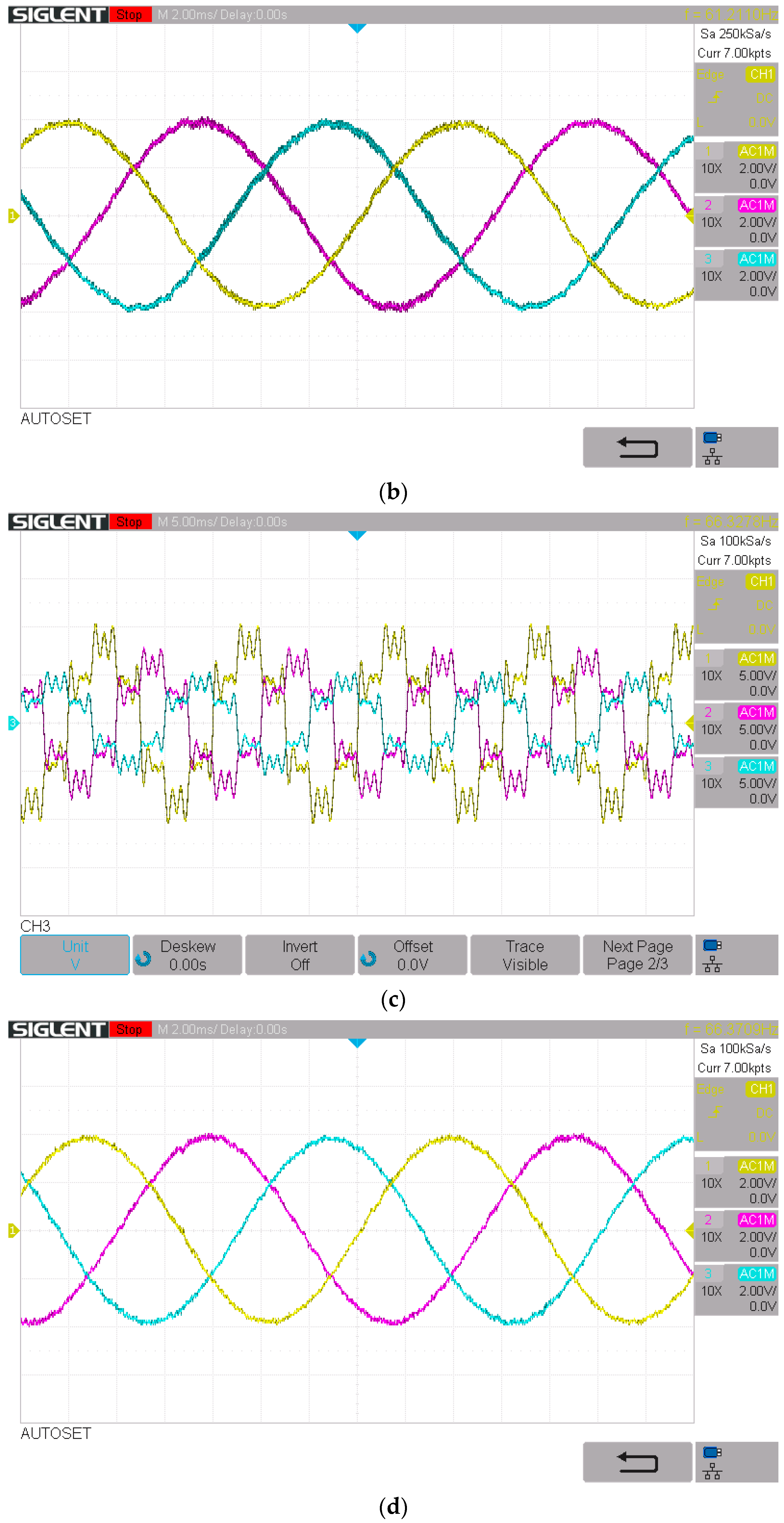
The results obtained in the real-time simulations mirror those obtained during the MATLAB/SIMULINK model simulations. The importance of using the digital simulator is that the tests are carried out in an environment that more closely resembles a real photovoltaic generator.

 ,
, 


