1. Introduction
Energy requirements have become one of the most concerning problems for the global environment nowadays [
1]. The total amount of energy consumed by the global market increased from 396.0 exajoules in 2000 to 604 exajoules in 2022, with the majority of energy consumed by non-OECD countries. It was reported that global energy consumption for all non-OECD countries increased by 2.4% from 2011 to 2021. Conversely, for OECD and EU countries, energy consumption decreased slightly by 0.2% and 0.6%, respectively. Encouragingly, the share of oil consumption worldwide dropped from 39% in 2000 to 31% in 2021, while the share of renewable energy consumption increased from nearly 0% in 2000 to 7% in 2021 [
2].
Another problem triggered by increasing energy demand is the surge of unwanted emissions including carbon, nitrogen, and sulphur oxides [
3]. Since the Paris Agreement [
4] had been claimed to restrict carbon emission in 2015, the carbon dioxide emissions only increased by 0.6% from 2011 to 2021 [
2]. But as for NOx emissions, the data provided by the World Bank showed that they increased from 2.72 trillion tons in 2010 to 3.02 trillion tons in 2020 [
5]. Such a surge (>10% increase rate in 10 years) of NOx emissions has attracted some researchers’ attention. Until 2023, the research on NOx emission reduction techniques has become one of the most popular research topics in the field of engine technologies.
Concerning internal combustion engine (ICE) technologies, the two most common types of engines modifiable for renewable energy usage are spark ignition (SI) and compression ignition (CI) internal combustion engines (ICEs). They differ in approaches of ignition and fuel supply. The SI engine is a type of engine in which the combustion process is triggered by a spark generated by a spark plug. And there is usually a carburetor attached to the SI ICE’s intake, which improves the even mixing of air and fuel before injection. The port fuel injection method is usually used for SI ICEs due to the requirements of smooth flame build-up and stable air–fuel mixing. This technique is the injection of an air–fuel mixture into the intake manifold rather than directly into the combustion chamber (direct injection technique). Spark ignition internal combustion engines commonly work on original or modified Otto cycles [
6]. And as for CI ICEs, the combustion process is triggered by the heat of the compressed air. Compression ignition engines commonly work on diesel or modified diesel cycles. During the intake stroke, only air or other kinds of carrier fluid inducted into the combustion chamber and the fuel will then be directly injected into the combustion chamber for compression ignition. Compression ignition internal combustion engines have higher compression ratios, which thus result in higher thermal efficiency and power output. But on the other hand, CI ICEs’ combustion progress is less even than that of SI ICEs, so the emissions of unburned hydrocarbons are higher if fossil fuels are used [
7].
The principle of hydrogen-fueled internal combustion engines dates back to the 1970s [
8], with the first H2-ICE prototype designed and built by Sir Francois Isaac de Rivaz of Switzerland in 1806 [
9]. The Miller cycle, proposed by Ralph Miller in 1957 [
10], involves adjustments to intake valve lift and timing profiles to isolate the compression stroke from the expansion stroke [
11], improving efficiency, reducing emissions, and enhancing power output, especially at high rotational speeds [
12]. However, hydrogen’s properties of low ignition energy and low density pose potential hazards of abnormal combustion, including pre-ignition, backfire, knock, and spontaneous ignition [
12].
Water injection techniques, known for their effectiveness in improving engine performance and preventing knock [
13], have been utilized since World War I and were further developed during World War II, mainly for high-output aircraft engines. Research by P. Xu et al. [
14,
15] investigated the combustion and emission characteristics of a hydrogen-fueled spark ignition engine with direct water injection, showing significant reductions in NOx emissions with increased water injection.
Lean-burn combustion, especially for spark ignition engines, has garnered significant research attention due to its potential to reduce negative pumping work and improve cycle efficiency. However, lean-burn combustion may increase NOx formation due to higher air intake.
Research by Z. Ran et al. studied the lean spark ignition combustion of various fuels, highlighting syngas’s stability under extremely lean conditions and its low lean misfire limit [
16]. Simulation studies by Li [
17] using a 1D Navier–Stokes equation solver and Realis WAVE software developed a dual-piston, two-stroke spark ignition engine with green fuel replacement and intake valve closure principles.
This study introduces an oxyhydrogen ICE model with direct water injection and early-intake valve closure (EIVC) technologies developed using Realis WAVE software. While some research exists on hydrogen applications in IC engines, few studies focus on oxyhydrogen combustion combined with water injection and the Miller cycle. The aim of this research is to conduct a simulation study in this area and investigate engine performance. The baseline model was validated and then modified into an oxyhydrogen-powered engine to eliminate emissions. Water injection was then applied to reduce the cylinder temperature and increase the gas mass within the cylinder. EIVC technology was also integrated for further improvements, resulting in an H2-O2-H2O ICE model capable of zero-emission exhaust and slightly better performance than the original gasoline-fueled engine.
3. Results and Discussion
The simulation results are organized, documented, and discussed in this section. Three models were developed in total. Initially, a baseline model was created and meticulously calibrated for accuracy. Subsequent progressive upgrades were implemented, each aimed at enhancing performance based on the analysed results obtained at each stage. Ultimately, the final model exhibited superior performance and emission characteristics compared to all other models.
3.1. Baseline Model
3.1.1. Brake Power Validation
Figure 6 shows the comparisons between the original 4-MIX engine experimental results and the baseline model’s simulated brake power with the increment of rotational speed. Specific results and errors are shown in
Figure 6b.
After conducting comparisons, it was ensured that all predicted brake power errors remained below 5% across all rotational speeds. Both sets of results reached their peaks at a rotational speed of 7500 rpm, precisely matching the rated speed of the 4-MIX engine. This demonstrates that the simulation model closely aligns with the operational principles of the original 4-MIX engine’s simulation. Both the experimental and baseline model simulation data exhibit downward trends at higher speeds. Practically, this trend arises from the high demand but inadequate supply of air, specifically, oxygen for combustion, at high engine speeds. In the simulations, this was simulated by increasing the frictional force at high rotational speeds, as described in
Section 2.4.1.
3.1.2. Brake Specific Fuel Consumption Validation
Figure 7 shows comparisons of brake specific fuel consumption (BSFC) between the 4-MIX engine and the baseline model with the increment of rotational speed. Specific results are tabulated in
Figure 7b.
From
Figure 7b, it can be seen that all errors were kept under 5% at all rotational speeds.
3.1.3. HC + NOx Emission Validation
Figure 8 shows comparisons of combined unburned hydrocarbon and nitrogen oxides emission (HC + NOx) between the 4-MIX engine and the baseline model. Specific results are listed in
Figure 8b.
As it can be seen from
Figure 8b, all errors are kept under 5% in all rotational speeds.
3.2. Hydrogen Combustion in Pure Oxygen
The original 4-MIX engine was fuelled with a standard petrol–oil mix (50:1). Utilising such a type of fossil fuel mixture and air as the oxidiser caused unwanted emissions, including nitrogen and carbon compounds. Both the fossil fuel mixture and the air are sources of those undesired elements. Thus, to ultimately eliminate them from emissions, principles of hydrogen fuel replacement and pure oxygen combustion were both applied to the baseline model. The upgraded model can therefore produce zero emissions, theoretically.
Figure 9 presents the oxyhydorgen engine model’s performance results at varying rotational speeds.
3.2.1. Baseline vs. Oxyhydrogen Models: Performance Comparisons
Figure 9a shows the energy input rate results of the baseline and oxyhydorgen models. Both of these lines are nearly straight, which show that the growth of energy input rate is proportional to the growth of rotational speed. Each 500 rpm increment of rotational speed can boost the increment of energy input for 0.5 kW. The energy input rate of these two models was controlled on a similar level (5.51 kW).
Figure 9c shows the change in brake thermal efficiency versus the change in rotational speed for both the baseline and oxyhydrogen models. Both lines show downward trends with constant gradients. The thermal efficiency of the baseline model begins from 20.54% at a rotational speed of 6000 rpm and then starts to fall until reaching around 16% at a rotational speed of 8500 rpm. The thermal efficiency of the oxyhydrogen model shows a similar trend to the baseline model. It starts from 19.33% at a rotational speed of 8500 rpm, which is slightly lower than the thermal efficiency of the baseline model at that speed. After that, the line of the oxyhydrogen model begins to drop and eventually overlaps with the line of the baseline model at a rotational speed of 8500 rpm. Generally, the difference between the two curves keeps falling as the rotational speed increases and it reaches its lowest level at a rotational speed of 8500.
Figure 9d presents the brake specific fuel consumption of both models. Both of these curves present bend-up tendencies. This tendency can be explained according to the reduction in thermal efficiency. A lower efficiency caused more energy to be wasted; thus, a higher fuel consumption rate was obtained. It is very apparent that the BSFC of the oxyhydrogen model is generally three times as large as that of the baseline model. This interesting multiplicative relationship can be ascribed to the multiplicative relationship of petrol and hydrogen’s heating value, as mentioned previously in
Section 2.1. The percentage differences were huge between these two models, mostly higher than 65%.
Figure 9b presents the brake torque curves of the baseline and the oxyhydrogen model at varying CAD. Generally speaking, both curves present upward tendencies. This can be explained by the reduction in brake thermal efficiency shown in
Figure 9c. However, the curve of the oxyhydrogen model decreases more gently; the increment of rotational speed at 2500 rpm only reduces the brake torque by 0.1 kW. At low and medium rotational speeds, the value of the oxyhydrogen model barely changes. And as for the brake torque of the baseline model, it falls as the rotational speed rises. Each addition of 500 rpm sees a reduction of 0.07 kW. The difference between the two curves is the largest when operating at a rotational speed of 6000 rpm and then decreases to nearly 0 at a rotational speed of 7500 rpm. After the rated rotational speed, the brake torque of the oxyhydorgen model eventually becomes higher than that of the baseline model.
3.2.2. Baseline vs. Oxyhydrogen Models: Temperature and Pressure Comparisons
Figure 10 presents comparisons of cylinder temperature and cylinder pressure.
In
Figure 10a, the cylinder temperature of the oxyhydrogen model is generally higher than that of the baseline model. During the compression stroke, which is in the range of 180 to 0 before top dead center (BTDC), the cylinder temperatures of both models rise gradually. After 10 CAD BTDC, which is the timing of spark ignition, both models experience dramatic increments of cylinder temperature. This is caused by the rapid combustion of fuels in a short period of time (30 CAD). It can be easily seen that the gradient of the baseline model’s curve is lower than the gradient of the oxyhydrogen model’s curve, which shows a higher combustion speed of hydrogen than the 4-MIX fuel (petrol and oil mixture). The baseline model reaches its maximum cylinder temperature of 3055.76 K at 19 CAD. However, the oxyhydrogen model reaches its maximum cylinder temperature of 2177.5 K at the same crank angle. And at the beginning of the exhaust stroke, which is at 180 CAD after top dead center (ATDC), the exhaust temperature of the oxyhydrogen model is 1882.69 K, while the exhaust cylinder temperature of the baseline model is much lower (969 K). The much-higher cylinder temperature of the oxyhydrogen model is due to the high flame temperature of hydrogen (around 3000 K under pure oxygen conditions and around 2300 K under standard air conditions) [
6]. The compression of the oxygen–hydrogen mixture also intensifies the combustion process, so the maximum cylinder temperature obtained was 3056 K.
Figure 10b presents variations of cylinder pressure versus varying CAD for both models. The curves of both models coincides for the most part. The main difference is located where both curves reach their peaks. Unlike their cylinder temperature, both curves of cylinder pressure reach their maximums at different CAD. The cylinder pressure of the oxyhydrogen model reaches its maximum of 46.21 Bar at 10 CAD. However, the baseline model comes to the top of its cylinder pressure 5 CAD later than the model and its maximum value is slightly lower as well (43.92 kW). The compression ratio of the models was unchanged, at 9.8. Thus, only minor differences in peak pressure values and timings were observed.
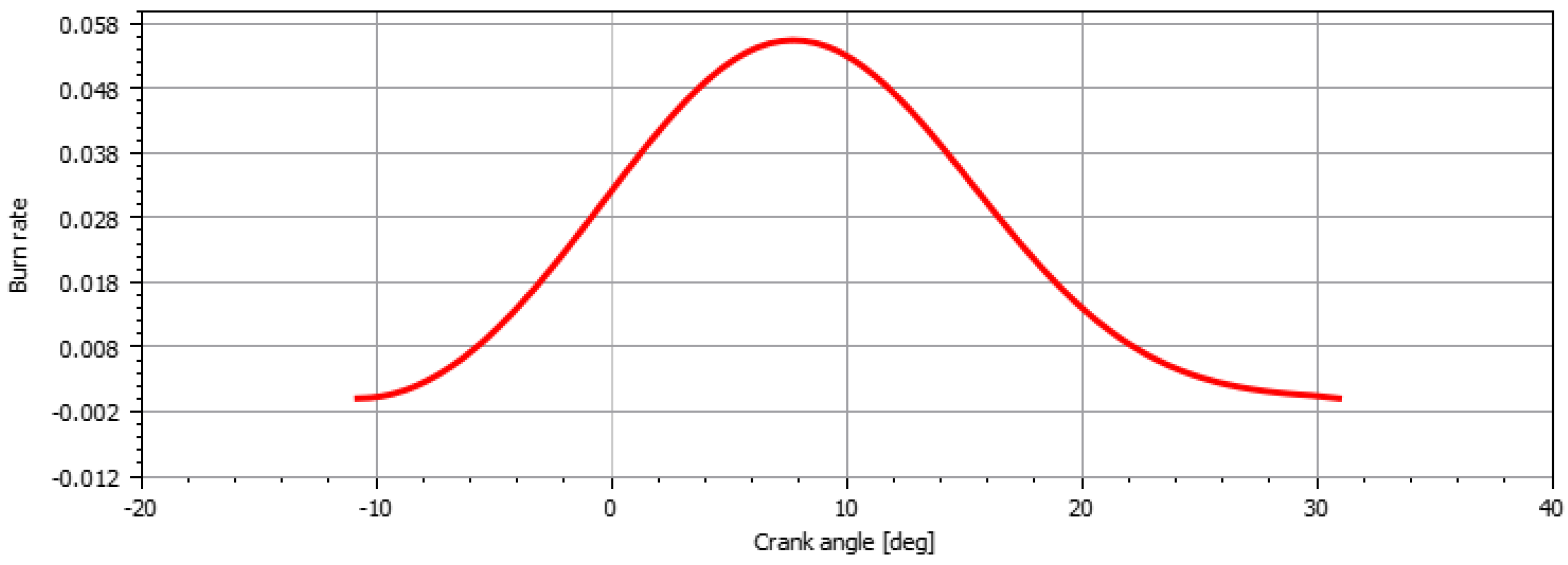
Figure 10c presents variations of the heat release rate versus carrying CAD for both models. After the timing of ignition, which is at 10 CAD BTDC, a significant difference can be seen between the models. The baseline model reaches its peak of 0.8 J/degree at 9 CAD ATDC and the oxyhydrogen model reaches its peak of 4.75 J/degree at 7.84 CAD ATDC. The figure shows the baseline and oxyhydrogen models’ difference in heating value visually.
3.2.3. Discussion
There is no doubt that the application of the pure oxygen combustion technique solved the most essential problem very effectively—the emission of unwanted gases. By using hydrogen instead of fossil fuel and using pure oxygen instead of air, unwanted emission including nitrogen and carbon compounds can be eliminated theoretically. But on the other hand, this technique also triggered a significant drawback, which is the abnormally high cylinder temperature. In most realistic working occasions, engine materials cannot bear such high cylinder temperatures lasting for the whole compression stroke (0–180 CAD ATDC). However, the exhaust temperature of the pure oxygen combustion model was too high as well (1882.69 K at 180 CAD ATDC). Also, due to the high heat value and low density of hydrogen, the mass of contents injected into the engine cycle was significantly reduced. This reduction in the mass injected into the cylinder lowered thermal efficiency of the system. Thus, further improvements are required to solve these newly discovered drawbacks.
3.3. Water Injection Application
There were two main purposes for applying the water injection:
- (1)
To reduce the general cylinder temperatrue and the exhaust gas; temperature
- (2)
To keep the total injected mass constant.
The determination of required injection rate of fuel, pure oxygen, and water were shown in
Section 2.6.
All simulations were carried out at the rated rotational speed of 7500 rpm, as it was determined that errors of energy input were nearly 0 at this speed in
Section 3.2.1.
3.3.1. Performance Analysis
Figure 11 presents the performance results for varying rates of water injection at a constant rotational speed of 7500 rpm.
Figure 11a shows how the rate of water injection affects the rate of energy input. It can be easily seen that the rate of energy input is approximately kept at a stable level.
Figure 11b presents the variation of brake torque versus the water injection rate. The brake torque decreases as the water injection rate increases when the rate of water injection is no more than 2.5 kg/h. After this turning point of 2.5 kg/h, the curve starts to grow as the rate of water injection increases. The percentage changes in brake torque are larger than the rates of energy input, but the turning point at 2.5 kg/h can be seen in both
Figure 11a,b.
Figure 11c shows the variation of the brake thermal efficiency versus the rate of water injection. It shows a similar shape to the previous curves. The curve shows a decreasing–increasing trend with the point of turning located at 2.50 kg/h. Before this turning point, the brake power drops as the rate of water injection increases. Then, it starts to increase until it eventually climbs to its maximum point of 1.21 kW with 6.28 kg/h of water injection. When compared to the baseline model, the brake thermal efficiencies were generally lowered when the technique of water injection was applied. But after the rate of water injection was raised above 5.02 kg/h, the brake thermal efficiency could be improved to a level higher than the baseline model’s.
Figure 11d illustrates the change in BSFC versus the water injection rate. It shows an opposite trend to the previous curves. The curve of BSFC begins from 0.16 kg/h without any water injection and starts to rise until reaching its peak value of 0.19 kg/h. Then, it starts to decline until it reaches a lower level, which was 0.2 kg/h lower than the original value of BSFC. The variation of BSFC shows a strong correlation with the variations of brake thermal efficiency, since the engine operating in lower efficiency requires a higher rate of fuel consumption.
3.3.2. Pressure and Temperature Analysis
Figure 12 shows variations of cylinder pressure and cylinder temperature. Water injection seems very effective in terms of cylinder temperature reduction. While no water is injected into the combustion chamber, which is the original situation shown in
Section 3.2, the peak temperature is 3243 K, and the exhaust temperature is 1977 K. While the water injection rate is increased from 0 to 2.5 kg/h, the technique shows dramatic influences on exhaust temperature. The effectiveness can be easily seen from two large gaps between the curves of 0 kg/h and 2.5 kg/h. This can be explained by the strong heat absorption ability of water during the gasification process. After that, the increment of the water injection rate keeps reducing the cylinder temperature to a minor extent, but not as strong as previously anymore. When it comes to the peak temperature, although the peak cylinder temperatures are all above 2800 K no matter how great a rate of water is injected into the chamber, water injection triggers a constant reduction in cylinder temperature after the point of peak temperature, which aims to control the cylinder temperature into a bearable temperature range. Because water was directly injected into the model after the combustion was nearly finished, the combustion environment inside the combustion chamber until the theoretical peak point was never changed; thus, the peak combustion temperature was not affected. But after the peak point, gasification of liquid water to vapour starts to take heat from charges; thus, the cylinder temperature then starts to decrease.
3.3.3. Discussion
It can be concluded that the effect of water injection depends on its rate. With a low water injection volume, water injection may produce negative effects on engine performances. But after the amount of water injection is raised over a certain value, positive effects of engine performance start to show up. The turning point can be roughly located at a water injection rate of around 2.5 kg/h. When the rate of water injection is lower than 2.5 kg/h, water injection can barely help with any engine performance characteristic. But after the rate of water injection increases over 2.5 kg/h, the technique starts to give improvements in engine performance. When 2.5 kg/h of water is injected into the combustion chamber, the exceeding cylinder temperature can be reduced to an acceptable level (<2000 K) in 28 CAD, which is 0.224 s in every cycle. Such a short time of exceeding cylinder temperature can be neglected and will not produce any hazards towards the safe operation of the engine. Overall, a water injection rate of 2.5 kg/h can be regarded as a point that meets halfway between engine performance and cylinder temperature management. This rate of water injection will therefore be used in the next model.
3.4. EIVC Miller Cycle Application
The main purpose of this group of simulations is to investigate the effectiveness of Miller cycle application, more precisely, the early-intake valve closure technique. The extent of early-intake valve closure was increased from 0% to 25% while the compression ratio was kept unchanged at 9.8. Thus, the expansion ratio was increased from 9.8 to 13.1.
All simulations were carried out at the rated rotational speed of 7500 rpm, and the rate of water injection in this EIVC Miller cycle model was set at 3 kg/h. That is possibly due to the application of high expansion ratio and EIVC enhancing the water gasification effect, which thus hinders the fuel combustion process at a high water injection rate. The results are presented in the following sub-sections.
3.4.1. Performance Analysis
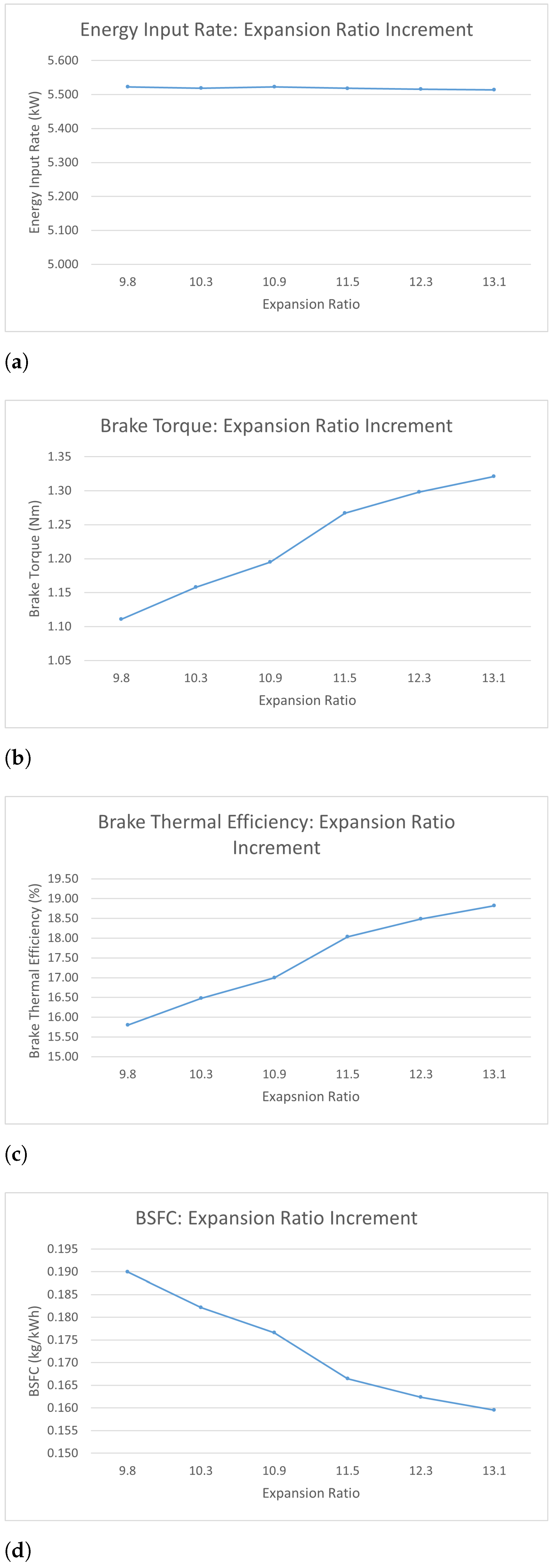
Figure 13 shows the performance results of the EIVC Miller cycle model with rising extents of early-intake valve closure.
Figure 13a presents the energy input results for varying expansion ratios. It is very apparent that the rate of energy input was kept in a stable range of 5.51–5.52 kW.
Figure 13b shows the variation of brake torque versus varying expansion ratio. Generally, it shows an increasing trend with all positive but fluctuating gradients. The curve starts from 1.11 Nm under the 0% early-intake valve closure condition, then it experiences a steady increment until its value reaches 1.19 Nm under the 10% early-intake valve closure condition. After that, the curve encounters a rapid increment of 0.08 Nm when the extent of early-intake valve closure is increased from 10% to 15%. Eventually, another steady increment can be observed when the extent of early-intake valve closure is increased from 15% to 25%. The curve shows the highest rate of increment between expansion ratios of 10.9 and 11.5, when 6.01% of brake torque is raised.
Figure 13c presents the variation of the brake thermal efficiency versus varying expansion ratio. Interestingly, the curve shows a very similar trend to the curve of brake torque. This phenomenon can be visually seen from comparing the values of percentage change in
Figure 13b,c. This phenomenon can be explained by the linear relationship between brake thermal efficiency and brake torque when the values of energy input are fixed at a stable level.
Figure 13d illustrates the change in BSFC versus varying expansion ratio. Overall, it shows a reversely proportional trend that decreases as the extent of early-intake valve closure increases. Eventually, the BSFC of the model is reduced to 83.68% of its original value.
3.4.2. Temperature and Pressure Analysis
As shown in
Figure 14a,b, the increment of early-intake valve closure and expansion ratio does not produce strong effects on cylinder temperature because of the unchanged fuel input rate and sufficient supply of oxidizer at all times. The maximum cylinder pressure increases by 35.86% comparing to its original value of 46.97 bar.
3.4.3. Discussion
Based on the performance results of all engines depicted in
Figure 13, a general rule can be inferred: engine performance parameters, including brake torque, brake thermal efficiency, and BSFC, show improvements as the percentages of valve opening profiles are reduced. The EIVC technique does not significantly affect cylinder temperature, but it notably increases cylinder pressure.
3.5. Overall Results Comparisons
All key parameters and the best results of all models are concluded and listed in
Table 1.
Figure 15a presents all models’ varying energy input rate versus changes in rotational speeds. Overall, all models show smooth increasing trends with minor differences. The EIVC model consumes fuel at the lowest rate among all models at all rotational speeds. After that, as the rotational speed increases, the energy input rates of all models go up in different gradients. When the rotational speed is around 7300 rpm, the energy input rates of all models except the EIVC model overlap at 5.4 kW. Generally, the EIVC model consumes 93.41% of the input energy of the baseline model on average.
Figure 15b shows the variation of brake torque versus the rotational speed of all models’ best results. Overall, the curve of the oxyhydrogen model presents an increasing trend and the curve of the EIVC model presents a decreasing trend. The curves of the baseline model and the water injection model show partial parabolic shapes. It is very apparent that the EIVC model’s data curve stays in the highest place among all models at all rotational speeds. And on the other hand, the water injection model’s curve stays in the lowest position among all models at all rotational speeds except 6000 rpm. At a rotational speed of 6000 rpm, the brake torque of the oxyhydrogen produces 0.806 Nm of torque, which is even slightly lower than the water injection model. At the rated rotational speed of 7500 rpm, the baseline model and the oxyhydrogen model overlap at the point around 0.996 Nm. At the same moment, the brake torque produced by the EIVC model is 38.65% higher than the overlapped value and the brake torque produced by the water injection model is 13.4% lower than the overlapped value.
Figure 15c illustrates changes in the brake thermal efficiency of all models at different rotational speeds. Still, the line of the EIVC model stays at the top among all models and eventually, it receives an improvement of 4.58% compared to the baseline model at a rotational speed of 8500 rpm. The line of the water injection model and the line of the oxyhydrogen combustion model start from the same point of around 19.3% brake thermal efficiency at a rotational speed of 6000 rpm. And after that, the difference between their values rises as the rotational speed increases. The line of the baseline model and the line of the oxyhydrogen model have a difference of 1.19% at the beginning of 6000 rpm. And then they start to approach each other as the rotational speed goes up. Finally, at a rotational speed of 8500 rpm, the baseline and oxyhydrogen models produce similar levels of brake thermal efficiency (around 16%).
Figure 15d shows the brake specific fuel consumption of all four models versus the increment of rotational speed. All models’ BSFCs gradually increase with the increment of rotational speed. Obviously, the baseline model burns fuel in the highest rate; it can be seen from the figure that the curve of the baseline model stands above those of the remaining three models, with a clear gap in between. This can be explained by the high heating value of hydrogen, as it can release thermal energy at a much higher rate than the mixture of petrol and oil (50:1).
4. Conclusions
In this study, a modified spark ignition oxyhydrogen-fuelled internal combustion engine Miller cycle with water injection application was proposed and simulated.
The main structure of the baseline model makes reference to an existing petrol-fuelled engine—Stihl 4-MIX 31cc. The layout principle of the simulation model refers to Li’s study [
17], with upgrades and refinments in the combustion and friction submodels. The results for brake power, brake specific consumption, and emissions were compared with the experimental results given by Knaus et al. for validation and calibration [
22]. They show that all simulation errors can be controlled in an acceptable range that is below 5%. And the simulation model shows its highest accuracy at a rotational speed of 7500 rpm, which is exactly the 4-MIX engine’s optimal rated working load. Thus, it is proved that the simulation model illustrates its accuracy of prediction in terms of engine performance and emission.
The oxyhydrogen model was modified based on the baseline model. In principle, the previous petrol-fuelled engine model was altered in terms of fuels, from a fossil fuel, petrol, into a renewable fuel, hydrogen. Also, the carrying fluid, air, was replaced with pure oxygen for the complete removal of the nitrogen and carbon elements contained in air. The replacement of fuels and carrying fluid aimed to eliminate emissions that are toxic to the environment (CO
2, NO, NO
2) and provide a potential source of water for the application of water injection. At the same energy input rate, the results of engine performance (brake torque, thermal efficiency, and BSFC) were compared with the baseline model’s. Both the baseline and oxyhydrogen model show descending trends, while the baseline model’s is relatively steeper, and the oxyhydrogen model’s is quite flat. At a rotational speed if 7500 rpm, which is the rated working load, both models produce a brake torque of 1.24 Nm. As for the brake thermal efficiency, the oxyhydrogen model’s results are generally lower than the baseline model’s, with an upper limit of 20% and a lower limit of 16%. When it comes to BSFC, a significant difference can be seen from the results. The BSFC of the oxyhydrogen model is around three times as much as the baseline’s. This can be explained by the fuels’ differences in heating value, as was mentioned in
Section 2.1. The cylinder temperature of the oxyhydrogen model is much higher than the baseline model’s, as well as the rate of temperature increment, since the flame temperature and speed of hydrogen are much higher than petrol’s.
The application of water injection aimed to not only reduce cylinder temperature, but also keep the mass input constant, since hydrogen is a fuel with a lower density but higher heating value than petrol. An additional water injector was attached to the oxyhydrogen model. The rate of water injection was calculated based on the principle of mass input constant. The rate of water injection was tried from 0 kg/h as the non-water injection condition to 6.28 kg/h as the exceeding mass input condition. Among all the results, including engine performance, cylinder pressure, and cylinder temperature, it was found that a water injection rate of 2.5 kg/h could be regraded as a turning point. When the rate of water injection was lower than 2.5 kg/h, increasing the rate of water injection produced negative effects toward engine performance but apparently positive effects toward cylinder pressure and cylinder temperature. Thus, the water injection rate of 2.5 kg/h was selected as meeting the halfway point between solving the hazard of excessive cylinder temperature and keeping the engine’s performance in an acceptable range.
When it comes the the model with Miller cycle application, based on the modification made in the water injection model with a water injection rate of 2.5 kg/h, the expansion ratio was increased from 9.8 in the baseline condition to 13.1 at maximum. Generally, a trend can be concluded that the increment of expansion ratio can produce positive effects towards engine performance. However, it does not produce noticeable effects on the combustion process and results while significantly raise the cylinder pressure.
In summary, the EIVC Miller cycle exhibited superior performance in terms of energy efficiency, torque output, and thermal efficiency compared to alternative models, effectively addressing concerns related to emissions and cylinder temperatures.
As for other progressive studies in potential, the problem of exceeding the cylinder temperature caused by hydrogen combustion can also possibly be solved by noble gas dilution. Due to noble gases’ characteristics of nonreactivity, the exhausted noble gas can be isolated from the mixture by condensation and then recycled for reuse. At the same time, the byproduct of condensed water can be used for the application of water injection as well. Possible drawbacks may include the accurate determination of mixing ratio and the occupation of space when it comes to commercial engine application. This novel principle based on the current results shown in this study will be further investigated in the future.


