1. Introduction
The global energy system is currently undergoing a transition towards a new paradigm characterized by decarbonization, the decentralization of generation, the electrification of the economy and a more sustainable use of resources. Thanks to technological advances and cost reduction, the implementation of electrical energy production systems is increasingly high. They represent a high percentage of the total power of the generation system and contribute to an increasing extent to the production mix of electric power. The increase in renewables as a share of energy supply in 2022 was the second largest in history. A total of 25% of the electricity generated worldwide was the responsibility of renewable photovoltaic and wind generation plants [
1]. Even faster increases are needed to align with the Net Zero Emissions Scenario [
2]. The European Green Deal establishes the pace of decarbonization required in the coming years [
3].
Electrical generation from renewable energies is associated with the resources (wind, photovoltaic) and is variable, intermittent and not dispatchable. Whilst the penetration of these generation sources is not high, they do not pose major problems for the operation and security of the electrical networks to which they are connected. But the high implementation of renewable energy is a challenge [
4]. High voltage variations and fluctuations or strong ramps may occur in the generation curves. This requires greater power capacity available in the electrical network and requires other flexible systems, both for generation and the response to demand.
In the planning process for new plants, power companies set limitations on the amount of power that can be connected. Relevant limitations are usually placed on the maximum power that can be injected into the network to limit these voltage fluctuations. The studies are usually conducted based on considering the most unfavorable situation for the system, that is, moments of very high production (the nominal power of the inverters is usually considered). However, such a high generation is produced in very few hours a year. This hinders the further implementation of photovoltaic plants, or the need to reinforce lines and substations. The operation of the electric companies’ assets is therefore very restricted since their capacity to conduct electrical energy is limited by the maximum values, and most of the time they are thus underused. But the maximum power is produced in very few moments a year, so the capacity of the networks is underutilized.
Owners of photovoltaic installations are also affected due to these characteristics of their systems. With the progressive increase in photovoltaic production during the central hours of the day, MWh prices tend to be very low precisely at the times of greatest production. This effect called “cannibalization” represents a reduction in its benefits, so its economic viability is compromised. At times when there is excess generation, curtailments are necessary, which further reduce its economic viability. These curtailments are becoming higher in some countries. On the other hand, energy generation from photovoltaic plants is subject to forecasting errors, which incur penalizing costs [
5].
Accuracy in long-term estimates of energy production, with time horizons greater than one year, is of utmost importance for the technical planning of future distributed generation (DG) units. An adequate estimate allows for the correct allocation of resources, the optimization of the infrastructure and the better integration of the DG units into the energy system. As baseload generation from the combustion of fossil fuels is replaced by renewable energy sources; ensuring reliable capacity firming support for the power grid will become crucial. Firm energy determines the maximum volume of energy that a generation unit can sell with a given level of reliability. The capacity value (or “capacity credit”) indicates the extent to which ERVs can be relied upon just like conventional power plants. The capacity value of solar photovoltaic (PV) is very low [
6,
7,
8].
The definition of the appropriate mechanisms to achieve the complete integration of renewable energies into the energy system is still under development. The selection of these mechanisms will depend on a variety of factors, including the climatic conditions of the area, policies implemented by the government, the specific geographical location and changes in costs that are revealed through techno-economic analyses [
9].
In this context, storage systems are positioned as a necessary technology to allow for the adequate grid integration of the growing renewable power. In order to move towards the net zero scenario, storage capacity must be significantly increased, reaching an annual average of 80 GW during the period between 2022 and 2030 [
6], and it is necessary to exploit different options. In particular, battery energy storage systems (BESSs) can offer such robust capacity, giving the system management capabilities for the generated PV energy. The storage industry is projected to grow to hundreds of times its current size in the coming decades. The dataset [
10] points to a considerable reduction in the prices of lithium-ion storage systems in utility applications over the last decade. The average cost has decreased from
$1659/kWh in 2010 to
$285/kWh in 2021.
Security of supply is a key factor in the electrical system. Installing batteries in parallel reduces overgeneration and the cutting and sale of energy during peak production hours. BESSs can offer firm capacity, providing the system with management capabilities for the generated photovoltaic energy. However, for economic reasons, it has been rare until now to discuss the operation of large-scale PV plants operating as baseload generation plants. From the point of view of hosting capacity, the power to be taken into account for the PV-BESS would no longer be the peak power of the collector field, but rather the constant power to be delivered to the network. This increases the number of facilities that fit into a given distribution network [
11]. For example, in Spain, the total nominal power of the distributed generators (DGs) should be less than 50% of the nominal capacity of the Medium Voltage/Low Voltage (MV/LV) transformer at the interconnection point [
12].
Another benefit of capacity firming is that the system and all its components operate close to their nominal power ratings for a longer time. Furthermore, the cost of converters in large-scale PV plants will be lower due to the power output smoothing that is supplied to the grid.
Unlike conventional substations, a substation for a large-scale PV plant has an uneven utilization coefficient due to the characteristics of solar radiation. BESSs can shift the peak of daytime photovoltaic production to the night. Furthermore, the capacity of the transformer of the substation connected to the photovoltaic plant can be decreased by directing the generation peaks of the solar panels towards the BESS [
9] for subsequent supply.
Due to all of the above, the concept of constant photovoltaic power generation (PV-CPG) arises to overcome these problems. The problems of voltage variations due to variable currents, ramps, the need for backup sources, the cannibalization effect, etc., are reduced.
References [
13,
14,
15,
16] accurately determine the optimal capacity of battery energy storage systems (BESSs) when integrated with renewable energy sources, taking into account the effects of battery degradation. Although the main thrust of these studies bears some resemblance to the present manuscript, they are not directly comparable. They focus on economic analysis. Our manuscript aims to completely abstract from economic analysis and focus exclusively on energy aspects. Furthermore, this model lacks comparability in terms of degradation, since the system does not provide a 24 h baseload.
In [
14], iterative methods are used, similar to the approach presented in this manuscript. However, it is important to note that the proposed degradation model is rather simplified and is based solely on another author’s model.
Study [
15] is consistent with our manuscript but focuses specifically on extremely fast charging stations.
The proposed system is designed to provide firm power or backup capacity to the electricity system. This steady flow of power from the generating plant is guaranteed with a high level of reliability. Therefore, its massive integration into the power grid could lead to a reduction in the need for frequency regulation technologies, as a high level of available power is guaranteed with reduced uncertainty. Some examples of firming power in the literature are the following.
In [
8], the goal is to achieve constant power output from 24 h to a few hours during the day. In [
17], a battery management and control algorithm mitigates fluctuations in intermittent PV generation for hourly periods. In [
18], the required energy storage capacity is estimated in order to guarantee the constant and reliable delivery of energy by wind and photovoltaic means in Japan’s electrical system.
A 50 MW AC PV system with 60 MW/240 MWh battery storage modeled in California can provide >98% capacity factor over a 7–10 p.m. target period with a lower lifetime cost of operation than a conventional combustion turbine natural gas power plant [
19]. However, this scenario is conservative, and it is not proposed to establish a 24 h baseload as proposed in the present study. In a similar way, in [
20], the storage is dimensioned for a large PV plant with storage in baseload operation.
In [
5], PV production is regulated with BESSs to maintain a constant output level, which significantly contributes to power grid stability, but only in a certain time interval during the day. In [
21], an analysis of the optimal relationship between the optimal size of the required battery and the peak power of the generation system is presented, as well as the optimal operating setpoint of a PV + STG system to provide firm capacity all year.
Given that the solar resource is notably lower in the winter months, a similar analysis was presented in [
22] but for constant operating setpoints on a monthly basis.
All these cases mentioned are conservative and do not propose to establish a 24 h baseload. They also do not take into account degradation phenomena in the BESS, as proposed in this study.
The present study is conceived within the framework of a planning phase for the electric grid and focuses on the technical optimization between a PV plant and the BESS, where the main requirement is the supply of a 24 h baseload generation of the system, defined as the production of constant and continuous energy 24 h a day. This means that the generation does not fluctuate and remains stable at all times, meeting the definition of baseload generation. In addition, a proven battery degradation model is integrated, and charge–discharge cycles are accurately calculated using the rainflow-counting algorithm to ensure reliable plant analysis.
The proposed study identifies the optimal dimensions of a PV plant hybridized with a battery energy storage system that supplies a constant power setpoint during monthly intervals. Through massive data analysis in a long-term simulation, indicators are generated that establish a relationship between the energy unavailability of the system and the BESS dimensions. Through an iterative calculation process, considering various operating instructions and system parameters, a comparative analysis is carried out with the purpose of determining the optimal installation size for each scenario.
The aging effects of lithium-ion battery storage systems have been considered, according to the curves offered by battery manufacturers. The replacement of the battery bank at the end of its useful life has also been taken into account.
This manuscript proposes an innovative and risky study that may not be economically feasible at this time. It therefore focuses on calculating energy balances and is conceived within the framework of a planning phase for the electric grid and focuses on the technical optimization between a PV plant and the BESS, where the main requirement is the supply of a 24 h baseload generation of the system, defined as the production of constant and continuous energy 24 h a day.
The remainder of this paper is organized as follows:
Section 2 presents the proposed model detailing its equations, phases, parameters and indicators. In addition, the modeling of the BESS degradation is included. The results of the simulation are shown in
Section 3. In
Section 4, conclusions are drawn.
2. Case Study
2.1. Problem Formulation
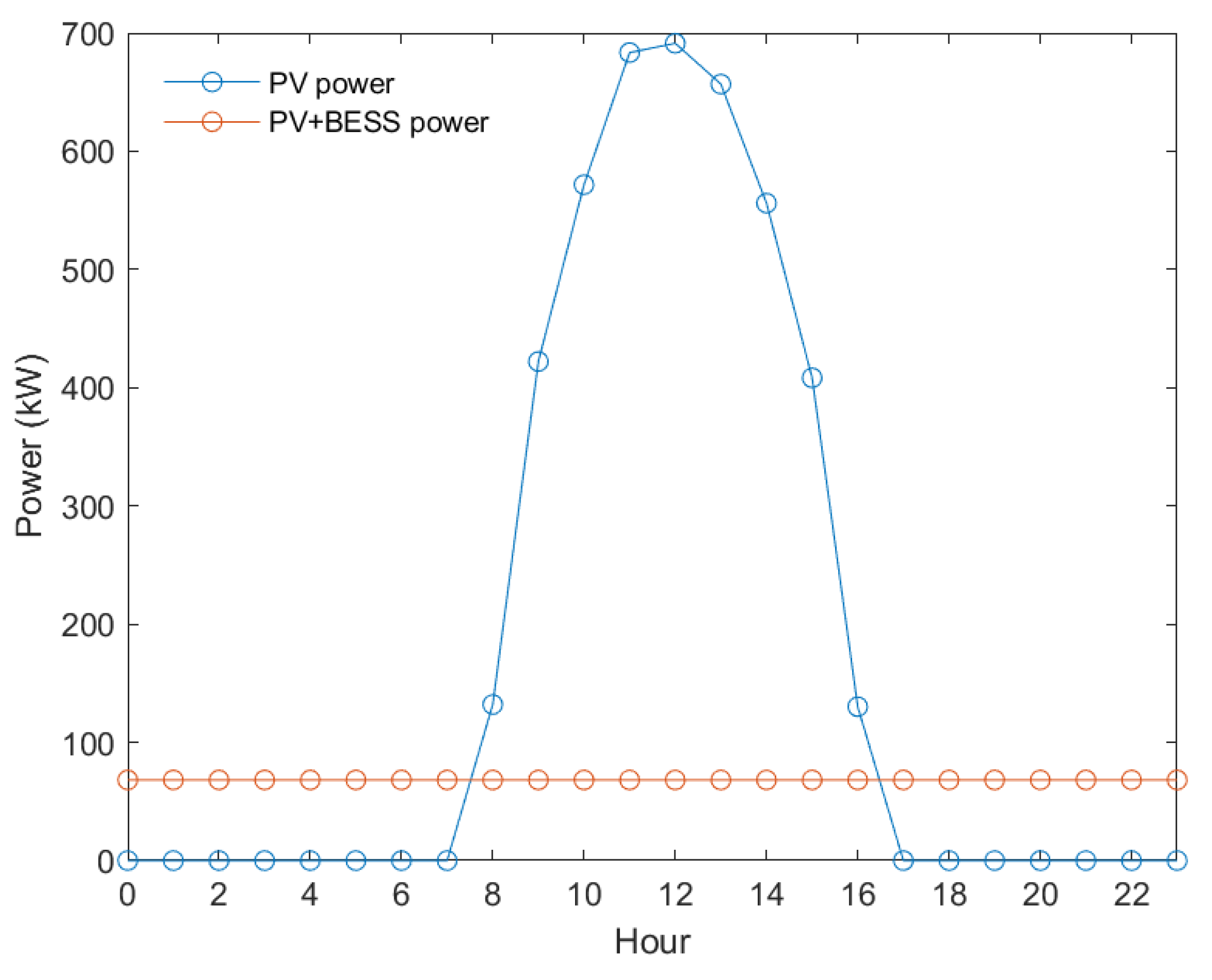
The aim is to transform a photovoltaic production profile, which has a characteristic bell-shaped shape, into a continuous and constant supply of power that remains uniform throughout 24 h a day with high guarantees of availability. A typical daily profile comparing both curves is shown in
Figure 1.
2.2. Proposed Model
In coherence with our previous research [
21,
22], the present study continues with the analysis of the behavior of a PV-BESS hybrid plant. The quantification of the BESS degradation and the appropriate assignment of the constant power are carried out for a correct evaluation of the system. The temporal frequency and the geographical point are fundamental components when defining the methodology of the study. Time frequency refers to the regularity with which data are collected and analyzed over time. The evaluation of large-scale PV plants, integrated into the electrical grid, can be achieved effectively through the use of hourly data [
23]. The short-term variability inherent to photovoltaic generation is mitigated by the periodicity of solar radiation over a broader set of time. The Sun exhibits cyclical patterns with a periodicity of around 11 years. For this reason, it is proposed to carry out a simulation that covers a period of 11 years starting from 2006. On the other hand, the geographical point refers to the specific location where the data are collected. In the present case, the School of Engineering and Architecture of the University of Zaragoza, located on María de Luna Street in Zaragoza, Spain, has been selected as the geographical point of reference. Since plant PV production is linked to the amount of solar irradiation, selecting a specific site involves collecting data for representative conditions unique to that region. However, it is possible to extrapolate the results to any region by modifying the irradiance data. Therefore, although the study is carried out in a specific location, its findings may have much broader relevance and applicability.
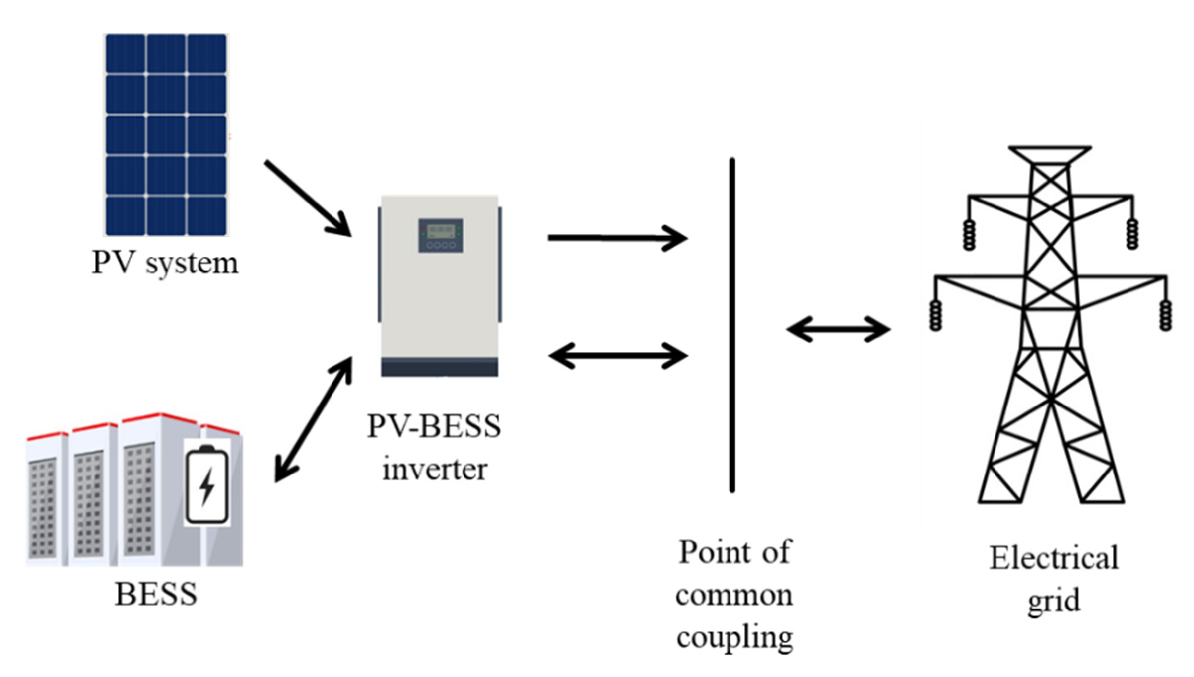
A simplified scheme of the proposed PV-BESS system is illustrated in
Figure 2. The photovoltaic plant transfers the generated energy to the electrical system through the inverter group. For its part, the energy storage system (BESS) has the capacity to inject energy into the system at times when the photovoltaic plant cannot satisfy the demand or, alternatively, to store the surplus energy generated by the photovoltaic system. It is imperative that, at the point of common coupling (PCC), a constant power setpoint is maintained to guarantee the reliability of the system.
By analyzing extensive photovoltaic production datasets, there is a tendency to neutralize fluctuations over short time horizons due to incidents or cloud cover. The algorithm developed in MATLAB R2021a classifies photovoltaic production according to months, thus identifying inherent seasonal patterns. In this way, the system power setpoint is adjusted monthly, based on the estimated photovoltaic production.
The efficiency of a PV-BESS is influenced by the power ratio between both components. Since the charging operation of the BESS is limited to the power generated by the PV plant, any power of the BESS that exceeds the power of the photovoltaic generation may be inefficient. Therefore, to avoid the underutilization of the BESS, a restriction is established that the power of the BESS must be less than the peak power of the photovoltaic generation (PBESS = 1 MW).
In the context of a preliminary theoretical analysis, the sizing of the BESS is addressed under a hypothesis of a daily balance between energy production and its supply. According to this model, the BESS is charged during peak daytime generation hours and discharged during the remaining hours to ensure the supply of a constant baseload. For the specific case of the location of this study, according to the PVGIS website [
24], it is determined that the average daily production of a PV plant is 4.36 kWh/kW. Therefore, for a 1 MW PV plant, the theoretical capacity of the BESS required to displace energy production at any time of the day would be up to 4.36 MWh. Therefore, the approximate C-rate of the BESS is 0.23.
2.3. Model Equations
In this paper, part of the model previously proposed in [
21,
22] is used. Following that, the equations that characterize the PV-BESS model are briefly described.
For the PV plant, 2041 Tallmax TSM-DE15V(II) 490W monocrystalline photovoltaic modules are selected, developed in China by Trinasolar for utility-scale PV applications [
25].
Using Equations (1)–(3), the photovoltaic production for each hour is obtained. PV output was simulated for fixed systems facing south at 35° tilt.
For an accurate assessment of PV production in a specific area, it is crucial to have long periods of irradiance data. This is because solar irradiance is subject to significant variations resulting from changes in meteorological and seasonal conditions. The long-term solar radiation data are analyzed for a period of 11 years, taking the hourly irradiance from the PVGIS database [
24]. The temperature reached by the PV cells is defined in Equation (1) when the module is exposed to operating conditions. This temperature is influenced by the ambient temperature and irradiance.
where
TC is the module temperature [°C].
TA is the ambient temperature [°C].
GM is the global irradiance incident [W·m−2].
NOCT is the Nominal Operating Cell Temperate [°C].
Equation (2) models how the power generated by a photovoltaic panel varies as a function of cell temperature and incident irradiance.
where
PMOD is the module PV power [W].
γ is the temperature coefficient of PN [%·°C−1].
PN is the nominal power of the photovoltaic module [W].
GSTC is the irradiance under standard measurement conditions [W·m2].
GM is the irradiance [W·m2].
Finally, using Equations (1) and (2), the hourly power production of the PV plant is calculated using Equation (3).
where
EPV is the hourly PV energy production.
NP is the number of PV modules of the plant.
CLOSS are the losses associated with the PV plant (p.u.).
TS is the time slot of 1 h.
The accumulation of losses is quantified with the C
LOSS coefficient of 13.4% [
26,
27,
28].
Using Equations (4)–(7), the energy stored in the BESS in each hour is calculated, taking into account the constraints and its equivalent model.
To adequately represent the energy balance of the BESS, the power restrictions specified in Equations (4) and (5) must be taken into account. PMAX is equivalent to EB,MAX since the maximum C-rate is 1.
The charging (
PBC,t) and discharging (
PBD,t) power of the storage system is
PMAX, which is equivalent to its capacity, since the maximum C-rate is 1. During the charging process of the BESS, the power constraint is determined by the difference between the production of the PV plant and the energy supplied to the grid. In the discharge process of the BESS, the power constraint is based on the difference between the energy supplied to the grid and the output of the PV plant.
where
PBC,t is the effective charging power of the BESS at the current time (t) in W.
PBD,t is the effective discharge power of the BESS at the current time (t) in W.
PMAX is the nominal power of the BESS in W.
PPV,t is the photovoltaic power supplied at the current time (t) in W.
PGRID,t is the power setpoint to be supplied to the electrical grid at the current time (t) in W.
The stored energy at the current time (
t) is related to the stored energy at the previous time (
t − 1) [
29,
30] according to Equation (6).
where
EB,t−1 is the capacity of the BESS at the previous time (t − 1) in Wh.
ηB,EF is the round-trip efficiency in p.u.
The efficiency (
ηB,INV) of Equation (6) varies in the proposed model depending on the power supplied. The efficiency of the conversion in the inverter has been taken from the Battery Energy Storage inverter Ingecon Sun Storage datasheet 100TL [
31]. Therefore,
Table 1 shows efficiencies for significant operating points with respect to the nominal power of the inverter that have been taken.
Self-discharge is measured as the charge lost over time and limits the energy available in the battery. The internal chemical reactions that contribute to self-discharge are mainly quantified when the BESS is not used for long periods of time. Due to the daily use of the BESS, the effect of self-discharge can be considered insignificant since the manufacturer of the BESS identifies 5 W of losses [
32]. Therefore, self-discharge phenomena are ruled out in the proposed model.
Regarding Equation (6), some operational limits related to the storage capacity of the BESS are established, which are identified from Equation (7). Although the BESS manufacturer indicates a 100% depth of discharge [
32], for safety, a depth of discharge of 90% is chosen (
DoD = 0.9).
where
EB,h is the energy stored in the BESS for each hour.
EB represents the energy exchanged in 1 h with the BESS in Wh. Positive if it is charging and negative if it is discharging.
EB,MAX is the upper capacity limit of the BESS in Wh.
EB,MIN is the lower capacity limit of the BESS in Wh.
EB,t is the hourly charging or discharging energy of the BESS at the current time (t) in Wh.
2.4. Model Phases
In the simulation process, a time step (Δt) of 1 h has been adopted. Consequently, all equations described in this section are evaluated at hourly intervals.
PV forecasting can be categorized into physical models and data-driven models. Physical models use numerical weather prediction, which shows good performance for forecast horizons from several hours to six days [
11]. To analyze long-term data, data-driven models are often used. Although the proposed algorithm is not based on machine learning, its approach is similar to data-driven models. It adopts a strategy that is based on the processing and analysis of historical data accumulated over an extended period. This approach is characterized by unraveling meaningful patterns and relationships within a dataset.
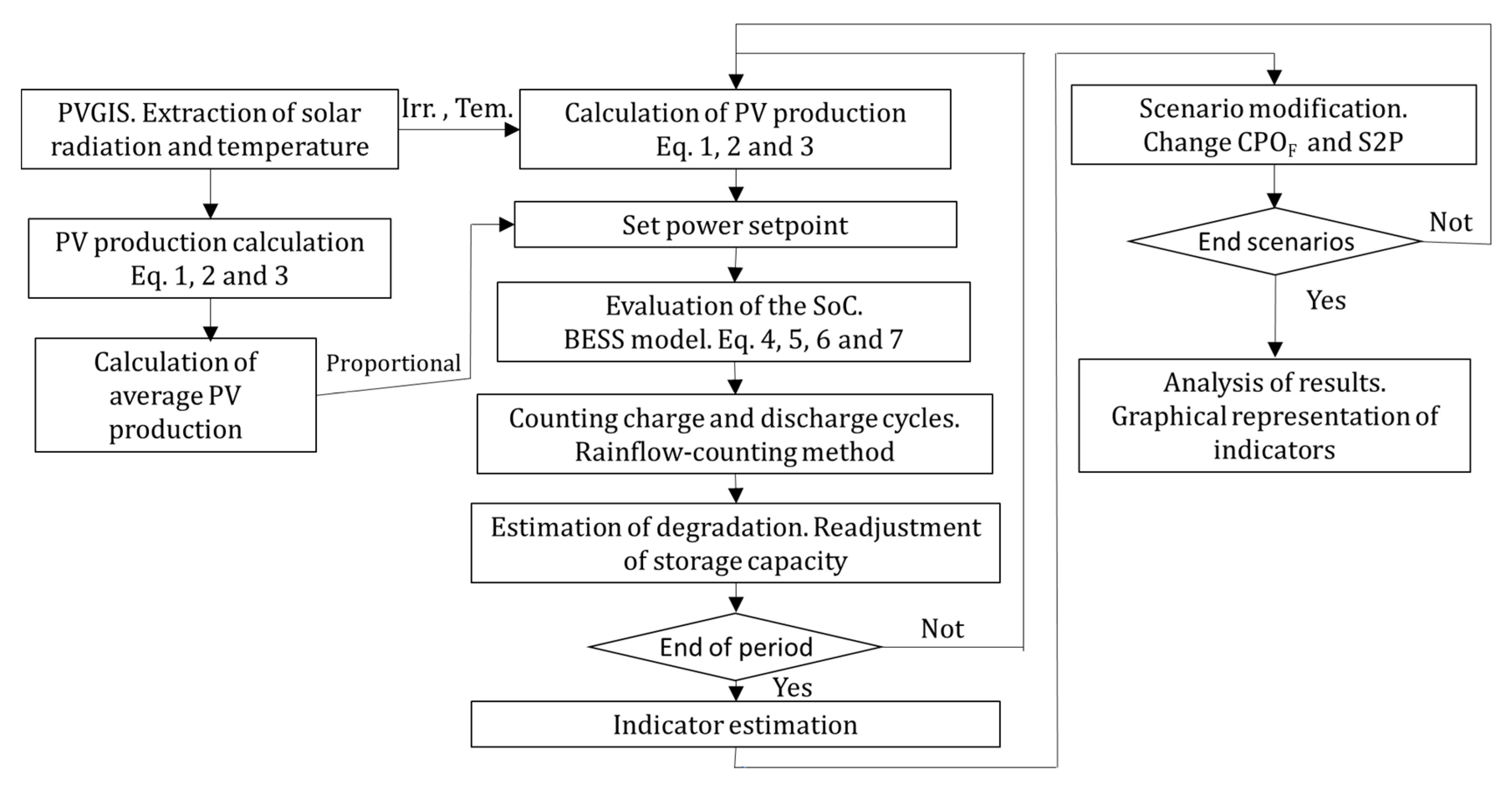
The algorithm in MATLAB is divided into two subsections to solve the problem, as shown in
Figure 3.
Left column blocks: As a preliminary step to the main simulation, a complete simulation of the time series is carried out using irradiance and hourly temperature as input variables. The hourly production of photovoltaic (PV) energy is determined for each hour of the simulation in order to calculate the average production of PV energy for each month of the year.
Center column blocks: The main simulation begins, in which, for each hour, the calculation of photovoltaic energy production is carried out based on the meteorological data provided by PVGIS. A constant power setpoint is established proportional to the average PV production of each month, obtained in the preliminary simulation. The SoC is calculated in the BESS according to its mathematical model. Charge and discharge cycles are counted by applying the rainflow-counting algorithm. Finally, the degree of degradation resulting from this cycling is estimated to adjust the capacity of the BESS. This process is repeated iteratively until the simulation is completed. At the end of the main simulation, the energy unavailability indicators are recorded. To identify significant operating points, the key parameters of the power setpoint and the size of the BESS are adjusted, thus repeating the main simulation. As a result, a matrix of indicators is generated based on parameters, which is used to graphically represent the results obtained.
2.5. System Parameters and Indicators
The specific parameters of the proposed BESS are provided in
Table 2 This table lists the characteristics of the BESS, including the rated capacity, voltage, efficiency and expected lifetime according to data provided by the manufacturer [
31].
One of the most important characteristics of any electrical power system is its rated power, that is, how many kW it can produce on a continuous, full-power basis. If the system has a generator, the rated power is determined by the rated power of the generator. If the generator were to deliver its rated power for a full year, then the energy supplied would be the product of the rated power times 8760 h/year. Since power systems do not run at full power all year, they output less than the maximum amount. The capacity factor (CF) is a convenient, dimensionless quantity between 0 and 1 that connects the rated power to the energy delivered [
33].
In Equation (8), the term CF represents the capacity factor, which is a dimensionless quantity between 0 and 1.
EGRID represents the energy supplied annually by the plant, while P
R is the rated power of the plant.
By the year of commissioning, the global weighted average capacity factor for new utility-scale solar PV reached 17.2% in 2021 [
34].
The S2P parameter defines the storage capacity of the system according to Equation (9) [
21].
CMAX represents the storage capacity of the BESS in MWh, and
PP is the peak power of the photovoltaic installation in MW.
S2P is a parameter equivalent to the number of hours of autonomy of a photovoltaic installation and is expressed in hours.
BESSs are designed to be versatile and easy to expand. The technical specifications for large batteries [
32] detail the capacity of each storage module. Specifically, the TS-IHV100E storage module by Tesvolt Lutherstadt Wittenberg (Germany) has a capacity of 80 kWh and allows four modules to be connected in parallel in a cabinet (total of 320 kWh).
Assuming that an S2P of 0.8 is to be selected and that the peak power of the PV plant is 1 MWp, the storage capacity of the BESS must be 0.8 MWh. This would require two full cabinets and an additional cabinet with two modules.
In Equation (10), the concept of the Constant Power Operating Factor is introduced [
21].
PGRID is the constant power that must be supplied to the electrical grid. This equation relates the power of the photovoltaic installation and the energy that must be provided to the grid. Therefore, the
CPOF parameter determines the equivalent operational performance of the system.
To ensure a constant and reliable energy supply, the system operation factor (
CPOF) must be lower than that associated with the average annual production of photovoltaic energy. If this requirement is not met, the photovoltaic installation will incur an annual energy deficit that the PV-BESS system cannot compensate. The
CPOF must be between 0 and 0.172 as mentioned for the average capacity factor previously. In Equation (11), the Annual Energy Deviation (AED) is defined as a relative accumulator of unavailable energy throughout the entire simulation period, where the numerator represents the unavailable energy, and the denominator represents the energy supplied throughout the entire simulation period [
26].
EPV represents the PV-BESS production for each hour,
EGRID represents the energy supplied each hour and h represents the number of hourly periods of the simulation. To obtain the average annual unavailability, the Annual Energy Deficit (AED) indicator will be used, which will take the average data of all simulation years.
In [
35], in order to determine the firm capacity of a distributed generation, a specific method is used that aims to obtain the minimum expected return on an investment, taking into account a pre-established confidence level. In accordance with the criteria established in the said study, a confidence level of 95% has been determined. Therefore, this study aims to guarantee that 95% confidence level. This means that the AED indicator should not exceed 5%.
According to data provided by the U.S. Energy Information Administration (EIA), in the period between 2013 and 2022, the capacity factor of nuclear power plants in the United States ranged between 90.8% and 93.4% [
6]. The guarantee of a 95% confidence level in the proposed PV-BESS equates its availability to that of a plant with the capacity to supply firm power in the electrical system.
The fundamental parameters of the BESS are evaluated primarily by Equations (12)–(14), presented in [
36]. It is common to use the SoC and SoH to estimate the energy performance, while the C-rate is used to approximate power performance. The SoC represents the current capacity in the BESS and is defined by Equation (12), where
QC is the content of the electric charge at the present state, and
QMAX is the maximum electric charge storage capacity at the present state.
The SoH represents the state of health of the BESS and is defined by Equation (13), where
QS is the maximum electric charge storage capacity in the specification, which indicates the fully charged battery capacity at the initial stage without degradation.
C-
rate is a parameter to describe the charging and discharge speed, which is calculated in Equation (14) where
I is the current.
2.6. BESS Degradation Modeling
2.6.1. Equivalent Cycle Estimation
As shown in
Figure 3, it is necessary to incorporate a degradation model for the BESS based on the accounting of charge and discharge cycles. The methodology that is usually presented to predict the useful life of batteries is based on situations where an identical charge–discharge cycle is repeated throughout the useful life of the battery. However, in most applications, the cycles change dynamically over time. In applications such as energy storage with renewable generation, daily variations in surplus generation lead to variability in the cyclic depth of discharge [
37].
To identify the operational behavior of the BESS, it is necessary to use a consistent method that adequately accounts for charge and discharge cycles.
The rainflow-counting algorithm has been widely used in research to analyze the fatigue and degradation of materials [
38]. This method identifies the loading cycles of a material subjected to fluctuating loads during its useful life. The algorithm allows for evaluating the durability of a component by estimating the stress levels necessary to produce fatigue failure.
Battery degradation is a complex phenomenon composed of several chemical processes. However, an analogy can be established with the fatigue phenomenon in materials. In both cases, part of the degradation process occurs as a result of the successive application of loads.
The method was first proposed by Matsuisi and Endo in 1968 and follows the ASTM [
39].
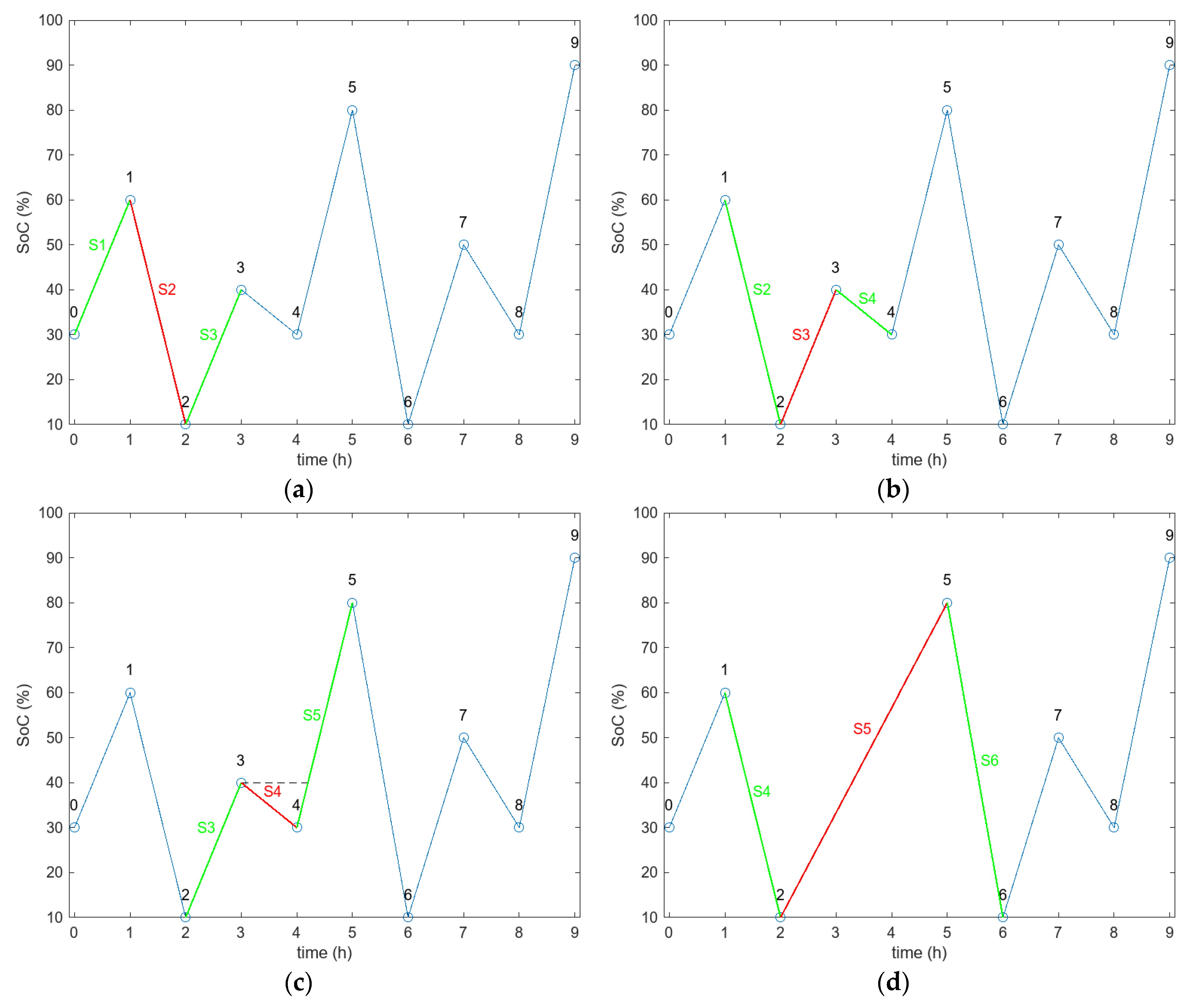
The algorithm counts the equivalent charge–discharge cycles from the time series corresponding to the state of charge (SoC) of the BESS [
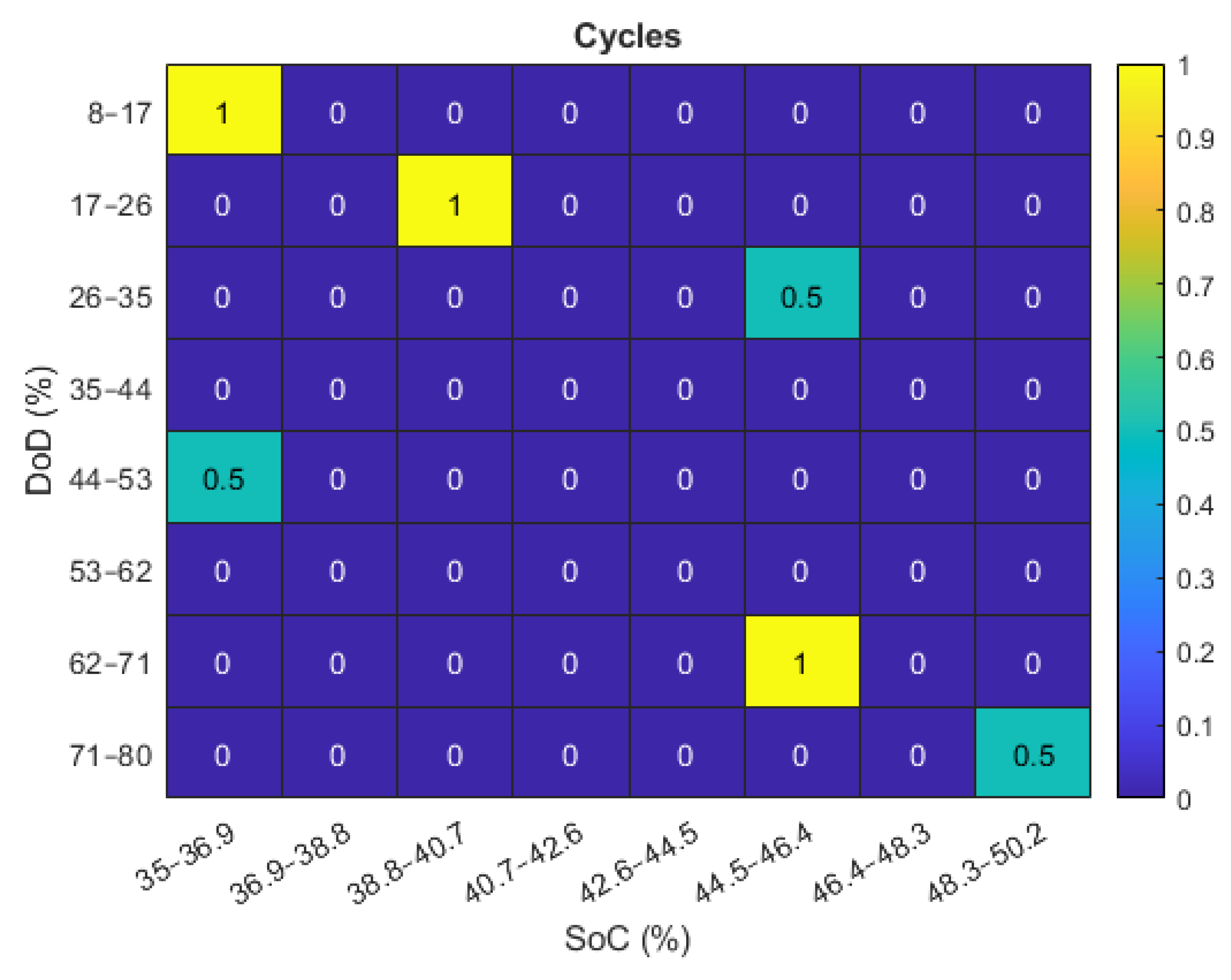
40]. To facilitate the understanding of the process, a theoretical explanation of the method has been combined with a fictitious example based on
Figure 4.
The procedure is listed below:
Each semicycle or cycle is classified according to its magnitude. The parameters that identify each magnitude are the average value of the path and the discharge depth. These parameters are essential to analyze the useful life of the batteries.
Table 3 shows all the half cycles or full cycles associated with the count in
Figure 4. The count column identifies a half cycle (0.5) or complete cycle (1). The range column represents the discharge depth of the BESS. The mean column represents the average SoC of each half cycle or cycle. The start and end columns identify each segment in the timeline.
In summary, this algorithm computed in MATLAB that applies the rainflow method to the proposed fictitious case in
Figure 4 has identified two cycles and five half cycles. The discharge depth and the average value of each section allow for a BESS degradation analysis to be carried out from a cycling point of view.
Figure 5 shows the number of equivalent cycles of the BESS as a function of the depth of discharge (DoD) and the average value of each cycle or half cycle, applying the rainflow-counting algorithm. The number of equivalent cycles is represented by a color scale, where yellow corresponds to a higher number of equivalent cycles. Each cell in the figure represents the number of equivalent cycles adjusted according to its amplitude and average value, since each component contributes a different weight to the BESS degradation.
In the simulations carried out in this study, the rainflow-counting algorithm is used to quantify the charge and discharge cycles in the battery.
In the Results section, cycling maps will be presented, similar to the example illustrated in
Figure 5, which classify and provide a concise visualization of the distribution of charge and discharge cycles throughout the entire simulation.
Previous experimental research has shown that deep cycling causes the most significant degradation, whereas smaller cycles are less significant [
37]. Thus, to achieve an accurate quantification of BESS degradation, it is necessary to determine the number of cycles for each level of discharge depth. Each segment represented in
Figure 5 generates a different level of degradation that will be quantified below.
2.6.2. Degradation Model of BESS
Batteries are electrochemical devices used to store and supply electrical energy. Due to the nature of their chemical composition, they are subject to a degradation process. The design, the electrochemical system, the temperature, the type of discharge and the storage period are factors that affect the useful life of batteries [
26].
There are different approaches to degradation modeling to quantify aging. Empirical models are based on data obtained through tests, semi-empirical models are based on data from aging studies and physicochemical models model aging mechanisms exclusively with differential equations. The simulations proposed to analyze the degradation in this paper are based on an empirical model supported by the tests carried out in [
41,
42].
Battery degradation is attributed to two independent components, known as cycling aging and calendar aging. In Equation (15), the term D
TOT represents the total degradation, while
DCAL represents the degradation attributable to calendar aging, and
DCYC represents the degradation related to the battery charging and discharging processes.
The factors that can influence each component are listed below.
Cycling Aging
To describe the degradation resulting from charge and discharge cycles, the term cycling aging is used. The main factors that contribute to increased degradation due to cycling aging are listed below.
Temperature (T): High temperatures cause cathode degradation and volume expansion, which accelerates the growth of the solid electrolyte interface (SEI) on the anode. Both causes are associated with a decrease in capacity and an increase in internal resistance [
43]. The Arrhenius equation states that the rate of a chemical reaction increases exponentially with temperature [
41]. Using Equation (16), the coefficient that relates temperature to degradation (
KCYC-T) is modeled.
KT is a parameter determined by empirical methods [
41],
TR is the reference temperature of 25 °C and
T is the ambient temperature.
Average state of charge (
): The (
) of a charge–discharge cycle has a slight influence compared to other factors such as the depth of discharge (DoD). In [
44], results are presented that indicate that carrying out cycling at high SoC ranges results in a significant loss of active lithium. This is due to the considerable expansion experienced on the surface of the graphite particles at a high SoC during the transition between the lithiation stages. As a consequence, the SEI layer on the surface breaks down and rebuilds itself irreversibly, leading to the consumption of active lithium. The relationship between this degradation coefficient (
KCYC-SOC) and the
SoC is modeled by Equation (17).
Kσ is a parameter that characterizes the sensitivity of the degradation determined in this equation.
Depth of discharge (DoD): It represents the difference between the SoC levels reached during a charge or discharge half cycle. It has been observed that as the degree of discharge (DoD) increases, more degradation occurs. High discharge values imply a greater risk of cracking and the formation of a new solid electrolyte interface (SEI) layer due to volume expansion in the graphite anode, especially when crossing the phase change regions in the anode [
44]. Empirical methods, such as [
35] and [
41], propose degradation models as a function of the DoD using exponential functions. In Equation (18),
KCYC-DOD represents the degradation coefficient as a function of the DoD, where
KBAT is the degradation constant provided by the manufacturer, δ is the DoD and
Kδ1 is a parameter identified empirically in [
45].
The K
BAT degradation constant can be obtained from the data provided by the manufacturer. In Equation (19),
DEoL represents the degradation per unit expected at the end of the useful life of the batteries (approximately 0.8), while
NCYC corresponds to the number of cycles necessary to reach this degradation.
Number of equivalent cycles (
NEC): Charging and discharging a battery does not always start with a 100% state of charge (
SoC) and end at 0% SoC, which would represent a full cycle. The NEC for a given DoD is defined as the number of cycles equivalent to a scenario where a full charge or discharge is performed in each cycle. The most pronounced aging mechanism is attributed to battery cycling, which involves graphite exfoliation, structural decomposition, transition metal dissolution and the growth of the solid electrolyte interface (SEI) layer. As a result of the factors explained above, the cycling aging component is obtained using Equation (20).
The resulting degradation does not follow a linear relationship. In order to fit the behavior of real cycling aging to the model proposed in this article, Equation (21) is used, which applies a non-linear relationship. K
1 and
K2 are the constants identified in [
41] to fit the model. The rainflow-counting algorithm method used is essential for quantifying the degradation due to cycling, since it provides information on the average value of the SoC, the DoD and the NEC.
Calendar Aging
The aging effects due to storage or the period of inactivity of the battery are called calendar aging. These effects are related to the loss of capacity due to the passage of time and are not independent of the charge and discharge cycles [
42]. The estimation of the degradation caused by the chemical decomposition of the electrolyte solution is clearly identified. Below are the factors that intensify the degradation related to calendar aging.
Temperature (T): Elevated temperature leads to the faster growth of the solid electrolyte interface (SEI) layer. This phenomenon accelerates cell degradation [
46]. The
KCYC-T factor of Equation (16) is valid to model this behavior.
Time (
t): Reactions due to SEI growth and binder decomposition increase over time. Even in the absence of charge and discharge cycles, the degradation mentioned in [
46] occurs. The
Kt factor of Equation (22) models this behavior by taking the constant
KC1 through empirical tests in [
41].
State of Charge (
SOC): If the battery charge level is high, there is a low potential at the anode and a high potential at the cathode. As mentioned in [
46], this low potential at the anode accelerates the growth of the SEI, resulting in the acceleration of the degradation. Furthermore, the oxidation of lattice oxygen is an electrochemical process that occurs mainly at high state of charge (SOC) ranges. This process results in a greater dissolution of the transition metal due to the oxidation of the lattice oxygen of the cathode [
47]. The
KCYC-SOC factor of Equation (3) is valid for modeling this behavior. As a result of the factors explained above, the calendar aging component is obtained using Equation (23).
As in cycling aging, for calendar aging, the degradation does not follow a linear relationship. To adjust the behavior, Equation (24) is used, which applies a non-linear relationship.
Table 4 presents the parameters used to identify the proposed degradation model, which are obtained from experimental results taken from [
41,
45,
48].
2.6.3. Issues with Lithium-Ion Batteries
The main limitations of lithium-ion batteries are the high price, lack of lithium supply and safety issues related to electrolytes.
The review article [
49] presents the main issues discussed in the literature on lithium-ion batteries. They are summarized below:
Increasing temperature has a significant impact on the accuracy of methods used to estimate the state of health, as well as increasing degradation in cells;
It is essential that proper heat dissipation methods are implemented in batteries. Failure to do so can result in reduced battery life, poor cycling performance and an increased risk of explosion;
Chemical separation processes for recycling face significant challenges on a large scale. Ethical and environmental concerns arise in the extraction of lithium, cobalt and other mineral resources, as well as issues related to their safe disposal;
Despite the efforts made in the research of cathodes, anodes and electrolytes, significant challenges remain. These include cathode dissolution, the negative effect of electrostatic interaction, dendrite formation, corrosion and passivation. These difficulties can lead to significant capacity degradation, low efficiency and short circuits;
Interface stability is a challenge because excessive overcharging or discharging, together with short circuits, causes cells to charge or discharge unevenly.
3. Results
The simulations carried out with constant power setpoints up to
Section 3.4 have been configured to maintain an intermediate value (CPO
F = 0.1). In [
21], simulations were carried out using various power setpoints, and it was identified that a CPO
F of 0.1 achieves an appropriate balance between the amount of energy supplied to the grid and viable energy unavailability, without the need to significantly oversize the BESS. If all the energy produced by the PV plant could be supplied, the capacity factor would be equivalent to the CPO
F power setpoint. In the Introduction, statistical data have been provided indicating that the average capacity factor in PV plants is 0.172. Therefore, it would not be feasible to supply power setpoints that exceed this value, and a setpoint with a CPO
F of 0.1 is a value close to the intermediate value.
In
Section 3.1, an initial approach is carried out to analyze the influence of each parameter on the degradation in the BESS.
In
Section 3.2, using the rainflow-counting algorithm, the model proposed in this study is simulated in order to analyze how degradation affects the cycling distribution in the BESS. The gradual degradation of the BESS has a significant impact on the fundamental degradation variables, which are the DoD and the
.
After analyzing the influence of each parameter on the degradation and distribution of cycles in the simulation, starting in
Section 3.3, results such as the predicted EoL and energy unavailability are presented. The purpose is to determine an appropriate installation size, taking into account variations in S2P and CPO
F.
3.1. Influence of Degradation according to its Parameters
The equations formulated in
Section 2.6 provide a mathematical framework to quantify the degradation experienced by a BESS due to cycling and calendar aging.
In this section, a simulation of the proposed model is carried out to analyze the influence of calendar aging and cycling. The results obtained confirm the validity of the model and ensure that the degradation is correctly estimated in subsequent simulations.
To achieve this, theoretical scenarios are simulated in which charges and discharges are applied to the storage system following cyclic patterns. The graphical results are shown in
Figure 6 and
Figure 7, where the state of health due to cyclic aging is identified. On the other hand,
Figure 7 shows the state of health due to calendar aging.
3.1.1. Cycling Aging influence
A simulation is carried out in MATLAB using the proposed model in order to analyze the influence of its main variables, the DoD and . In this theoretical scenario, the variables DoD and remain constant throughout the simulation, which implies that periodic charge and discharge cycles with identical magnitudes are performed. A constant temperature of 25 °C is assumed, to make the temperature variable independent of aging. The results obtained identify the influence of each variable on the gradual loss of battery capacity with each cycle.
Figure 6 shows a comparison of the SoH up to 10,000 cycles, for three cases with different cycling.
The blue curve in
Figure 6 is taken as a reference, with a DoD of 30% and
of 45%. In this system, symmetrical charges and discharges are carried out in the range of SoC values from 30% to 60%. The simulation corresponding to the blue curve in
Figure 6 modifies each variable with an increase of 40% to analyze which of them has a greater influence on the degradation.
In the first case, the orange curve in
Figure 6 represents a simulation in which the DoD is increased by 40% with respect to the blue reference curve. Symmetric charges and discharges are carried out in the range of SoC values ranging from 10% to 80%. Since this curve shares the same
as the blue curve, it isolates the influence of the
and facilitates the verification of the significant relationship between the degradation and the depth of discharge. The SoH after 10,000 cycles in the blue reference curve is 94.32%, and by increasing the DoD by 40% in the orange curve, the SoH drops to 82.25%. These results support the hypothesis that the DoD has a substantial impact on the degradation phenomena mentioned in
Section 2.6.
In the second case, the yellow curve in
Figure 6 with a DoD of 30% and
of 85% represents a simulation in which the
is increased by 40% with respect to the blue reference curve. The system performs symmetrical charges and discharges in the range of SoC values ranging from 70% to 100%. Only the
has been modified in comparison with the simulation of the reference blue curve, thus allowing for the influence of the
to be analyzed. The SoH after 10,000 cycles in the blue reference curve is 94.32%, and by increasing the
by 40% in the yellow curve, the SoH only drops to 92.16%.
The conclusion drawn is that the influence of the DoD is more significant than that of the but both must be taken into account for the cycling degradation analysis.
To estimate the degradation, it is common to propose a cycling aging model based on the DoD and
variables, using the rainflow-counting algorithm for cycle counting [
28,
33].
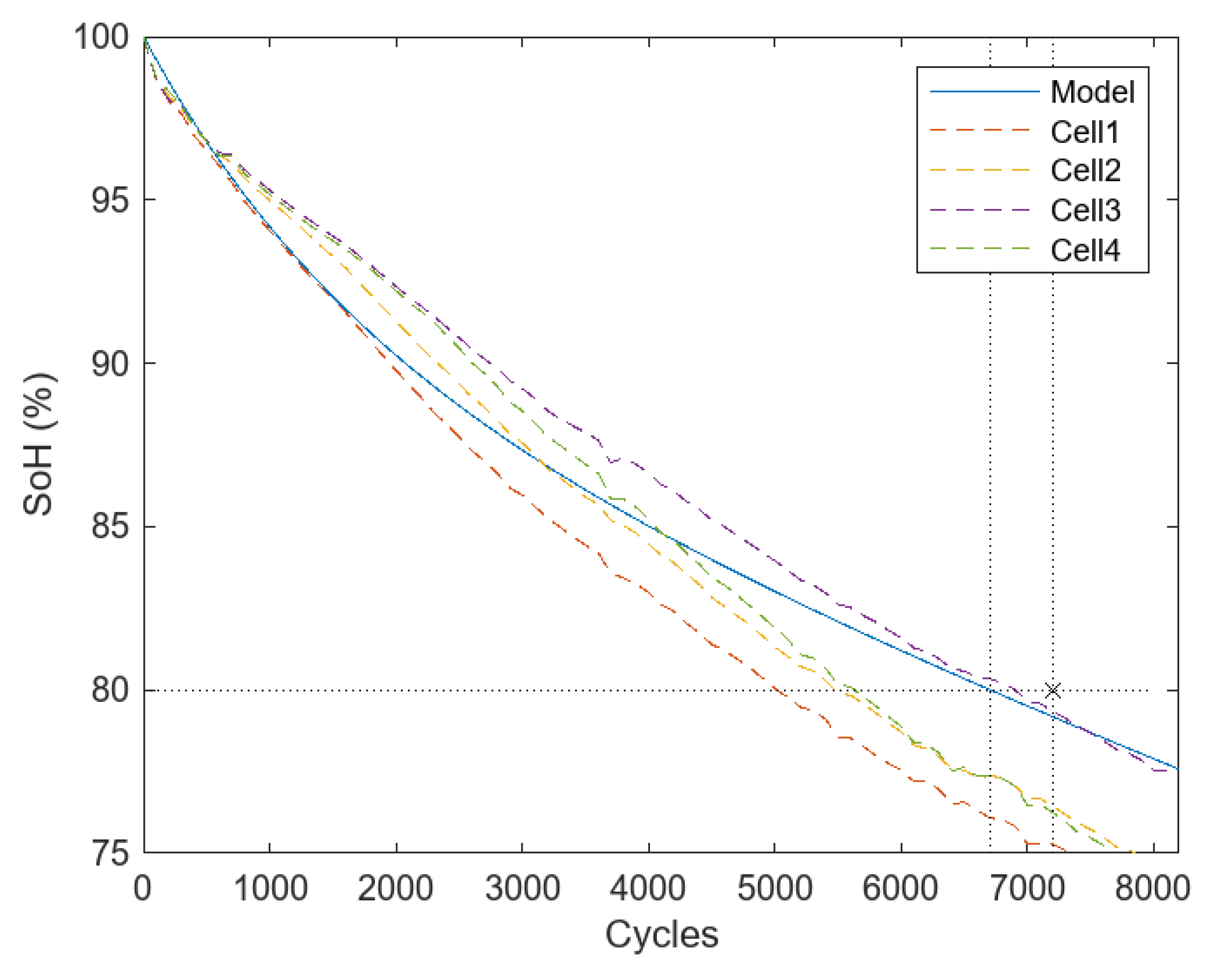
To validate the proposed cycling aging model, it is compared with long-term aging tests of lithium batteries. An industry reference dataset from the Oxford University Research Archive [
44,
50] is used. This dataset contains a long-term battery aging test for lithium-ion cells.
Figure 7 shows a graphical representation of the SoH or degradation as a function of the number of battery cycles. The blue curve with a solid line corresponds to the proposed model, while the curves with dashed lines represent the degradation of four types of batteries in the dataset [
44,
50].
It can be seen that the degradation levels in
Figure 7 are comparatively similar, although not identical. It is complex to identify an exact degradation pattern for each battery. Based on this observation, it is considered that the proposed model has substantial validity in predicting the degradation process until the End of Life or a SoH of 80%.
To validate the experimental model, a comparison is made with the data provided by the manufacturer of a commercial battery. The Lithium Iron-Phosphate PowerBrick battery datasheet [
51] presents the number of cycles vs. depth of discharge graph. For the curve with a DoD of 90% and a C-rate of 0.25 C, which resembles the average value of the proposed simulation, 7200 useful life cycles are identified.
According to the manufacturer’s specifications, the service life of the battery is considered to cover up to 80% of the initial capacity. Therefore, in
Figure 7, the End of Life according to the manufacturer has been identified with an “x”.
In the proposed model, the intersection between the limit value of 80% and the blue “model” curve in
Figure 7 identifies 6700 equivalent cycles, which is similar to the real value provided by the manufacturer. The data are compared with a Lithium Iron-Phosphate battery, because the composition of this type of battery has been used in large-scale BESSs such as [
32].
3.1.2. Calendar Aging Influence
The equations formulated in
Section 2.6 on calendar aging allow for the degradation to be quantified, considering both the passage of time and the SoC value. Several simulations are carried out in order to validate the proposed model, assuming that there is no cycling of the battery and the charge level is kept constant.
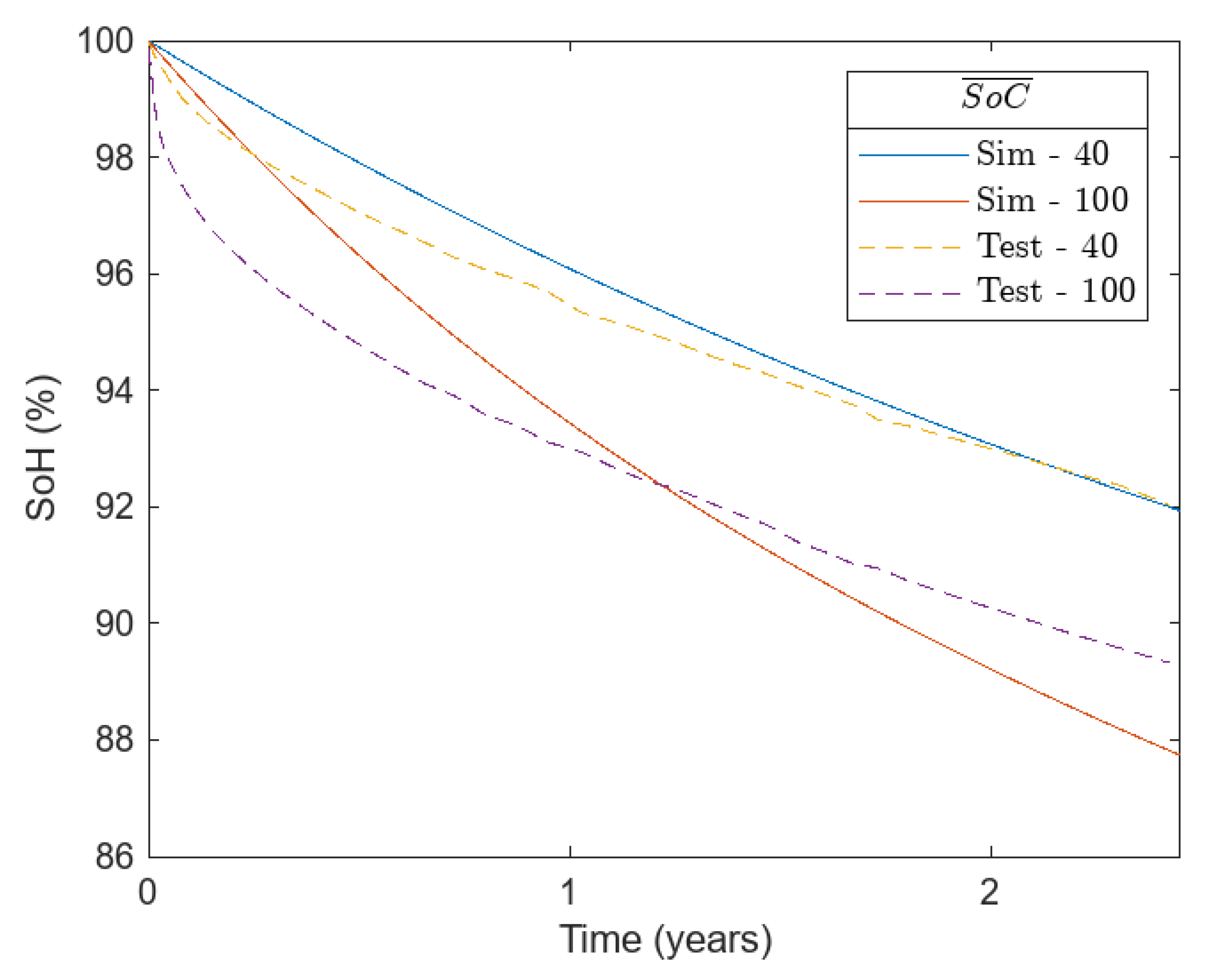
Figure 8, with the legend “sim”, shows the calendar aging caused by the proposed model. Compare with a degradation dataset obtained in [
52] whose legend in
Figure 8 is “test”.
Note that the higher the average state of charge
, the greater the degradation. After 2.5 years, the calendar aging simulation estimates a SoH of 88% when the SoC is 100%. However, the SoH is 91% when the SoC is 40%, as shown in
Figure 8.
To corroborate the aging calendar, degradation data of a lithium-ion storage system are presented in [
53]. It is observed that the degradation experienced coincides with that represented in
Figure 8 after approximately 2 years. For an SoC of 40%, an SoH of 92% is reported in [
53]. This figure coincides with the value represented in
Figure 8, where it is also observed that for an SoC of 40%, there is an SoH of the order of 92%. For an SoC of 100%, the SoH in both cases is around 90%.
Another relevant aspect is that the calendar aging is more pronounced during the first years of the battery’s life. The simulations represented in
Figure 8 coincide in showing a higher level of degradation around the first year.
In addition, a comparison of this model with a commercial battery is carried out. Taking the Lithium Iron-Phosphate PowerBrick battery [
51] as a reference, the manufacturer establishes in its specifications a calendar life greater than 10 years. Therefore, upon the expiration of this period, the End of Life is considered to have been reached, which results in a reduction in the storage capacity to 80%. In other words, the degradation is estimated to be equivalent to 20%.
For the equations proposed in the model of this article, the projection of an SoC of 80% would reach an End of Life at 8.7 years and for an SoC of 60%, at 10.7 years.
Therefore, it can be concluded that the calendar life of the proposed model is consistent and similar to the manufacturer’s specifications when average SoC values between 60 and 80% are considered.
3.2. The Influence of Degradation on the Cycling Distribution in the BESS
The introduction of degradation in the proposed model leads to a significant alteration of the BESS cycling process, since it causes a gradual decrease in its capacity. One of the most significant facts is the progressive degradation that affects the deeper discharge cycles, preventing them from reaching their maximum level. This implies that the BESS operation strategies are modified due to a capacity limitation.
Two simulations of the proposed model are carried out with the aim of analyzing its behavior until reaching the End of Life of the BESS, technically defined as 20% degradation in relation to its initial capacity.
3.2.1. Cycling Analysis for Reduced BESS Size
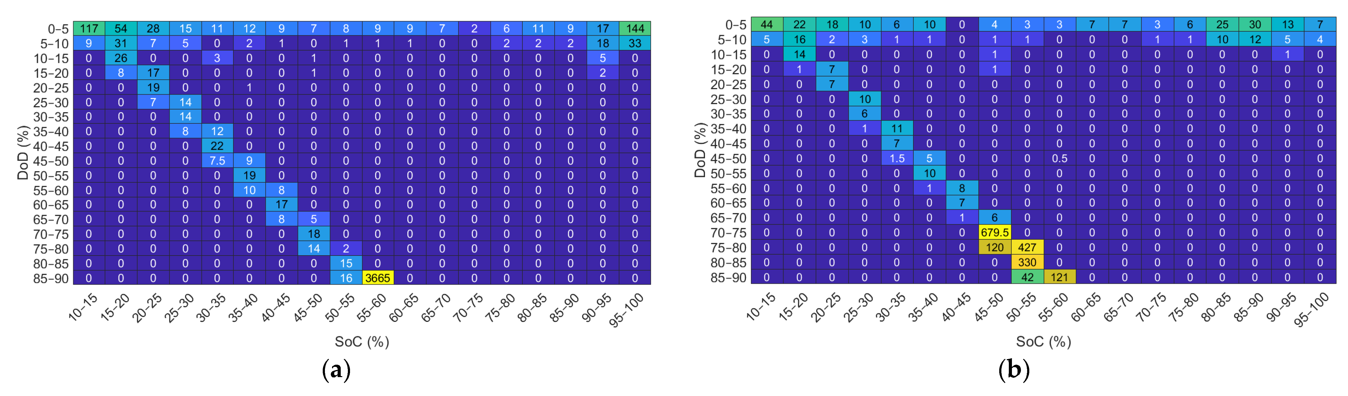
A relatively small storage size is chosen to ensure that the battery undergoes a full charge or discharge cycle in each operating cycle since its small capacity brings it to a state of full charge or discharge quickly. In this way, it is possible to systematically observe how high discharge depths, which are around 90%, experience a substantial reduction.
Figure 9 shows the behavior of the BESS through the analysis based on the count of load cycles (rainflow-counting algorithm). As observed in
Section 2, the charge cycle count is an essential metric in the characterization of the BESS.
Figure 9 provides a visual representation illustrating how each cycle occurs in the BESS.
Figure 9a shows a distribution of the charging cycles in which it is observed that the highest concentration of these cycles is around a DoD close to 90%. Additionally, the SoC is estimated at approximately 55%. Consequently, during each operating cycle, the system experiences a variation in the SoC that ranges between 10% and 100% of its total capacity. Specifically, the BESS has been subjected to 3665 operating cycles in this operating range. The rest of the cycles, compared to the magnitude mentioned, are numerically smaller and can be considered insignificant. This situation arises because the BESS has a relatively limited nominal capacity. Consequently, during any energy transfer process, whether charging or discharging, the BESS tends to reach its maximum capacity or be completely depleted.
Figure 9b incorporates the aging until its End of Life, which occurs at 44,352 h. Only during the first operating cycles of the BESS is it possible to reach maximum depths of discharge of 90%. Due to the manifestation of degradation phenomena inherent to the use, the ability to reach such a DoD decreases. This development reflects the importance of considering aging phenomena in a BESS.
In
Figure 9b, the aging phenomena are taken into account until its End of Life, which occurs at 44,352 h. It is only during the first operating cycles of the BESS that it is possible to reach maximum depths of discharge of 90%. Due to the manifestation of degradation phenomena inherent to the use, the capacity to reach such a DoD decreases. This development reflects the importance of considering aging phenomena in a BESS.
In
Figure 9b, it can be seen that the dominant distribution of operating cycles has changed in relation to
Figure 9a. Most of these cycles are now concentrated around 80% DoD and 50%
. It is noted that most DoDs start around 90% and decrease to around 70%. This indicates that, over the life of the BESS, it is operating in a DoD range that begins near its maximum capacity and gradually decreases over time as the battery degrades.
The observed situation has both positive and negative implications for the BESS. It is beneficial that, by operating with a smaller DoD, the phenomena of cycling aging are reduced. However, there is a progressive limitation on the capacity of the BESS. This restriction can lead to increases in energy unavailability in the system.
The degradation of the BESS constitutes a significant restriction in terms of its storage capacity, as observed in
Figure 9, and, consequently, its effects are interesting to analyze in relation to the parameters of unavailability of reliable energy throughout the time.
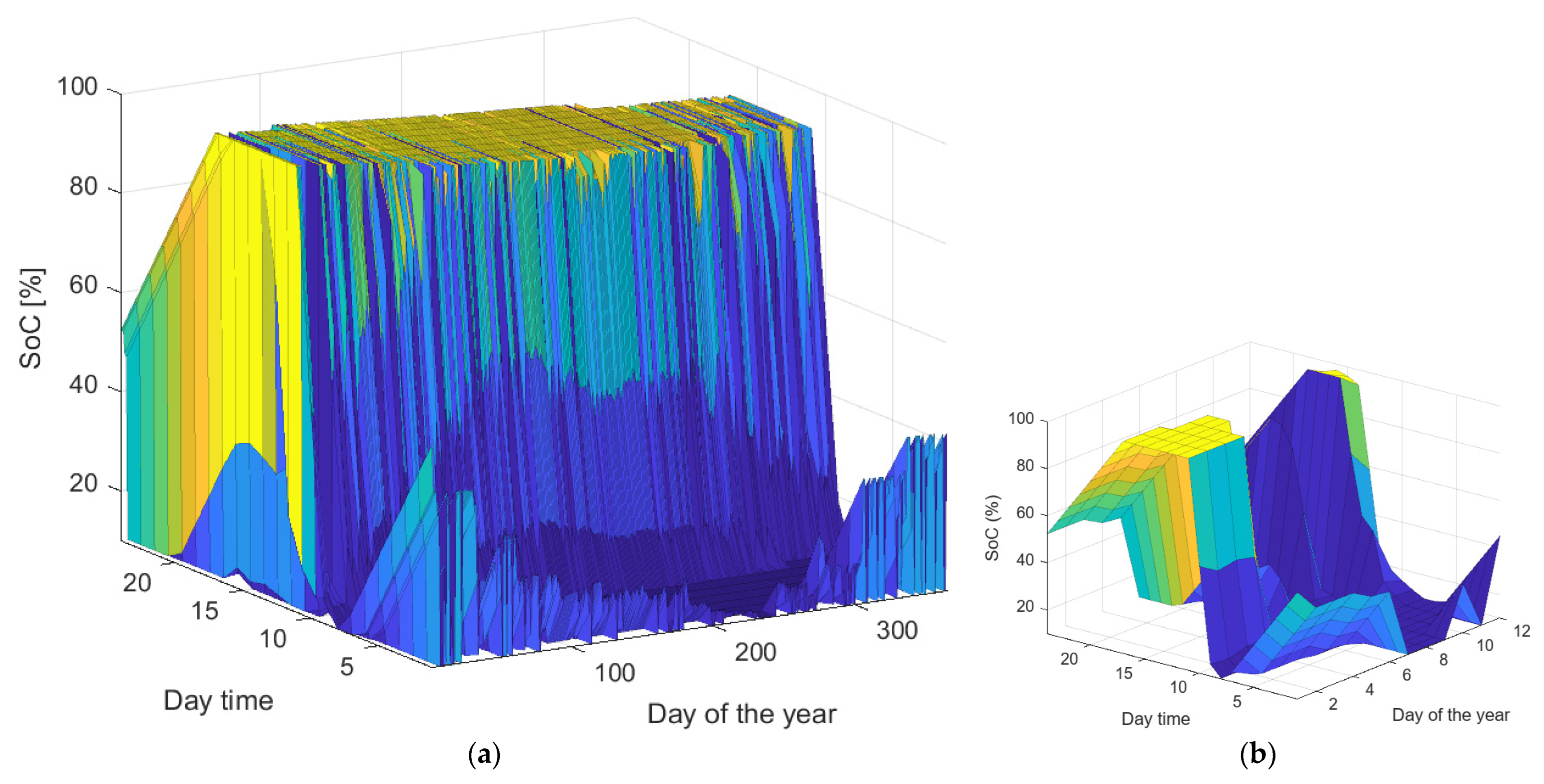
To obtain a perspective of the evolution of the energy levels in the BESS in this simulation,
Figure 10a is presented. The 3D graph illustrates the annual evolution of the resulting SoC during the operation of the BESS. It shows the day of the year on the “x” axis (day of the year), the sample number of each day on the “y” axis, which are the hours of the day, and the SoC on the “z” axis. In a small capacity battery, the SoC is fully charged and discharged most of the time. For days without PV production, the SoC remains fully discharged, as seen on day 8 of
Figure 10b.
3.2.2. Cycling Analysis for Oversize BESS Size
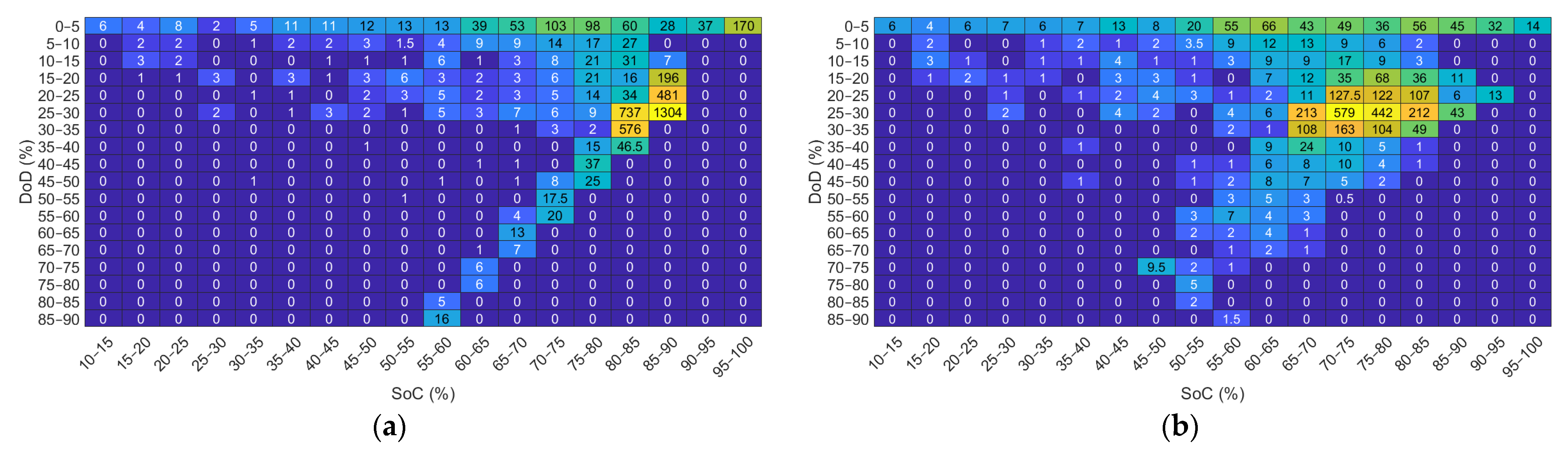
Figure 11 shows the distributions of the load cycles associated with an oversized BESS (S2P = 5). This situation contrasts markedly with
Figure 9.
In a hypothetical context where BESS degradation was not a factor to consider, it is observed in
Figure 11a that the majority of the cycles are concentrated around a relatively low DoD, approximately 30%. Additionally, the SoC remains at a high level, around 85%. Consequently, in each operating cycle, the system goes through fluctuations that range between 70% and 100% of its total capacity. These data suggest that, under these theoretical conditions, the BESS operates mostly in a higher range of its capacity, avoiding deep discharges and maintaining a high charge level. The rest of the cycles, compared to the magnitude mentioned, are numerically smaller and can be considered insignificant.
Figure 11b shows the aging phenomena until their End of Life, which occurs at 69,344 h. The dominant distribution of operating cycles has changed in relation to
Figure 11a. Most of these cycles are concentrated for a DoD of 30% and a SoC ranging between 60% and 80%.
Although degradation phenomena reduce the storage capacity, the degradation tends to be mitigated since the is reduced. This suggests that over the useful life of the BESS, it is operating at a DoD of 30% and around 70%.
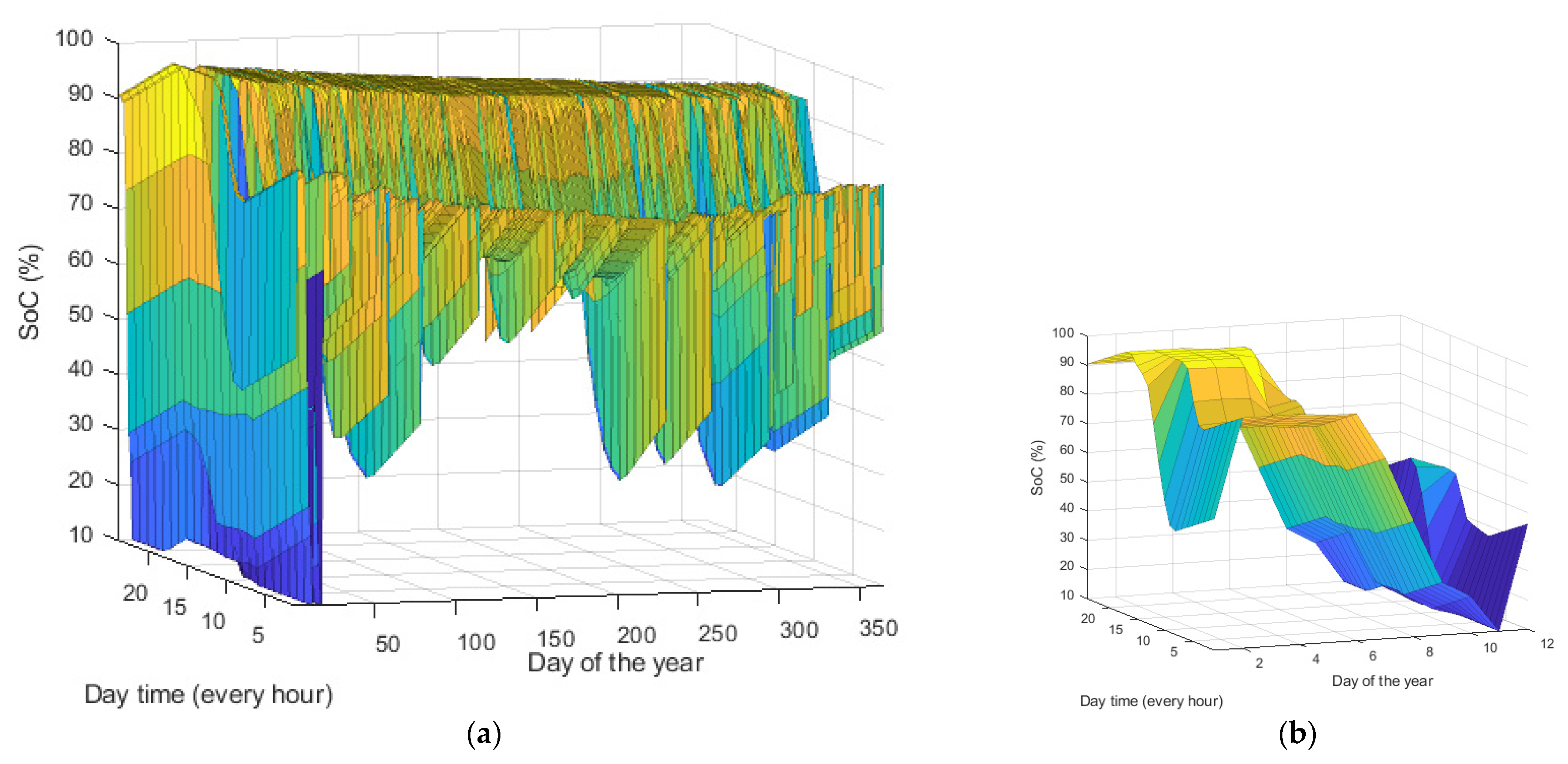
Figure 12 shows the evolution of the energy levels in the BESS for this specific case. Most of the time, the SoC is at levels close to 100%, and only occasionally after several days of low production does the SoC reach its minimum value, as can be seen in the zoom to
Figure 12b.
3.3. The Influence of the Size of the BESS on its End of Life
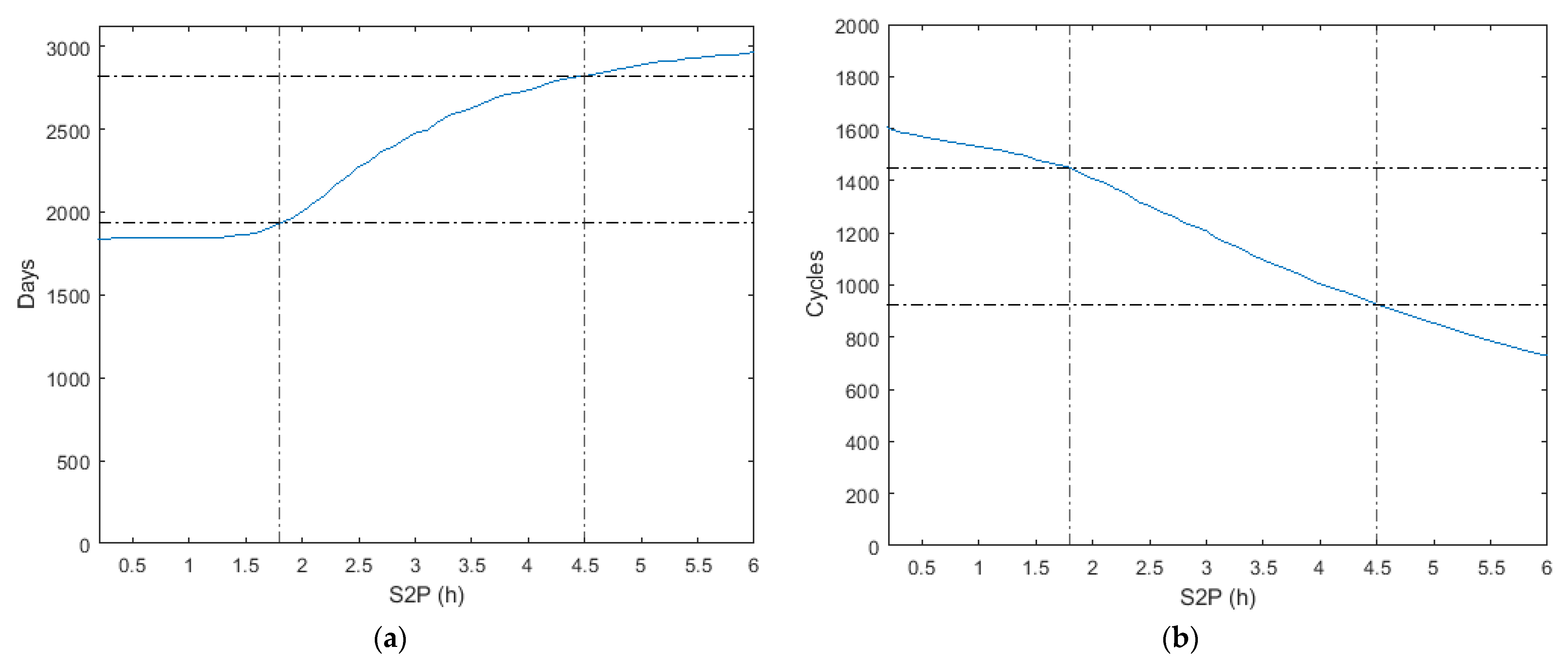
In the previous section, it was observed that the choice of BESS size has a significant effect on degradation. In order to determine the life of the BESS, the number of days until the BESS reaches the End of Life for each value of the S2P indicator is presented in
Figure 13a. This graphical representation provides information on how different BESS sizes affect system longevity.
In
Figure 13a, it can be seen that when selecting an S2P of up to 1.8, the degradation behavior is uniform, reaching the EoL approximately after 1875 days of operation. This specific feature is attributed to the limited storage capacity of the BESS. The storage system remains inoperative at its capacity extremes, either at maximum capacity due to a high PV generation or at its minimum capacity when there is no PV production, and the BESS is immediately discharged. It is important to highlight that these operating conditions are not valid in this study from the point of view of the energy unavailability of the system because the AED indicator exceeds 5%.
By increasing the storage capacity, and in particular when an S2P value of 1.8 is exceeded, battery charging and discharging processes operate with a lower depth of discharge (DoD). This implies that, in each cycle, the BESS does not use its full capacity, which has a direct effect on reducing the degradation rate of the cells. Consequently, the durability of the system benefits from the point of view of the degradation due to cycling.
This relationship is clearly manifested in
Figure 13a; as the S2P increases beyond 1.8, the time to reach the EoL extends linearly.
Starting from an S2P of 4.5, an inflection point is observed in
Figure 13a. Beyond this value, the increase in time before reaching the EoL tends to plateau, regardless of how much S2P continues to increase. Having an excessively high storage capacity, the BESS is frequently subjected to slight charge and discharge cycles that produce low cycling degradation. Instead, the system mostly remains in a fully loaded state. This scenario with such a large S2P size is also not realistic, since it implies the excessive oversizing of the BESS.
When a larger storage is selected, a decrease is observed in the total number of cycles that the BESS performs until it reaches its EoL. As seen in
Figure 13b, for a system with a more restricted capacity, specifically with an S2P of 1.8, the rainflow method, used to count charge and discharge cycles in storage systems, indicates that the BESS can support up to 1400 cycles equivalents up to their EoL. For a system with a larger storage capacity, with an S2P of 4.5, it presents an equivalent cycle reduction, supporting only 910 cycles until its EoL.
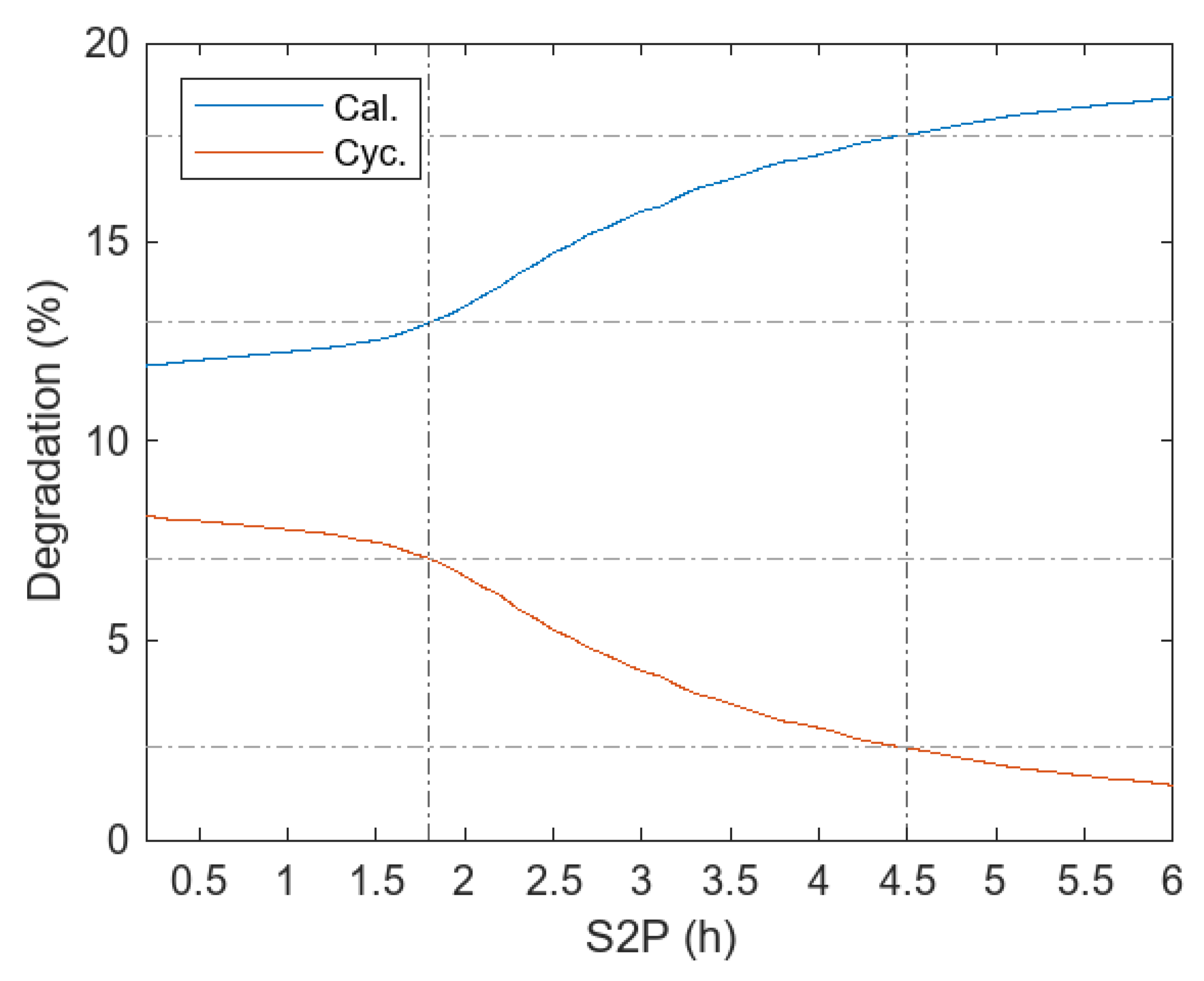
As mentioned in
Section 2, the degradation of the BESS is due to calendar and cycling effects. In order to determine the specific influence of each of these effects in the analysis proposed in this section,
Figure 14 shows the degradation curves corresponding to each of them as a function of the S2P parameter.
Figure 14 shows that calendar degradation increases with S2P. As the BESS capacity increases, it is observed that the SoC level remains high for longer periods of time. This behavior leads to further degradation per calendar. This correlation is corroborated with the calendar degradation study presented in
Figure 8. In this study, it is observed that a higher state of charge (SoC = 100%) generates considerably greater degradation compared to a lower state of charge (SoC = 40%). The relationship between the BESS capacity, the duration of high SoC levels and the consequent degradation due to scheduling is coherently reflected in the results obtained, highlighting the direct influence that system capacity has on these effects.
In terms of cycling degradation,
Figure 14 shows that an increasing S2P results in less degradation. This phenomenon is explained by the fact that a greater storage capacity implies charge and discharge cycles with a lower discharge depth. As previously discussed in
Figure 6, the depth of discharge is the main factor in cycling degradation, and the lower it is, the lower the cycling degradation of the BESS. Therefore, it is confirmed that the behavior observed in this case coincides with the theoretical model previously analyzed in
Figure 6.
Two sizes of BESSs are identified in
Figure 14. A reduced storage capacity (S2P = 1.8) presents a degradation due to calendar aging of 13.1% and due to cycling of 7%. On the other hand, for a BESS with high storage capacity (S2P = 4.5), the degradation by calendar is significantly higher than that by cycling. By calendar aging it increases up to 17%, while by cycling it is reduced to 2.6%.
3.4. Selection of BESS to Guarantee High Availability of Firm Power
The AED indicator, used in studies [
21,
22], has made it possible to quantify energy unavailability in a system similar to the one proposed in this work.
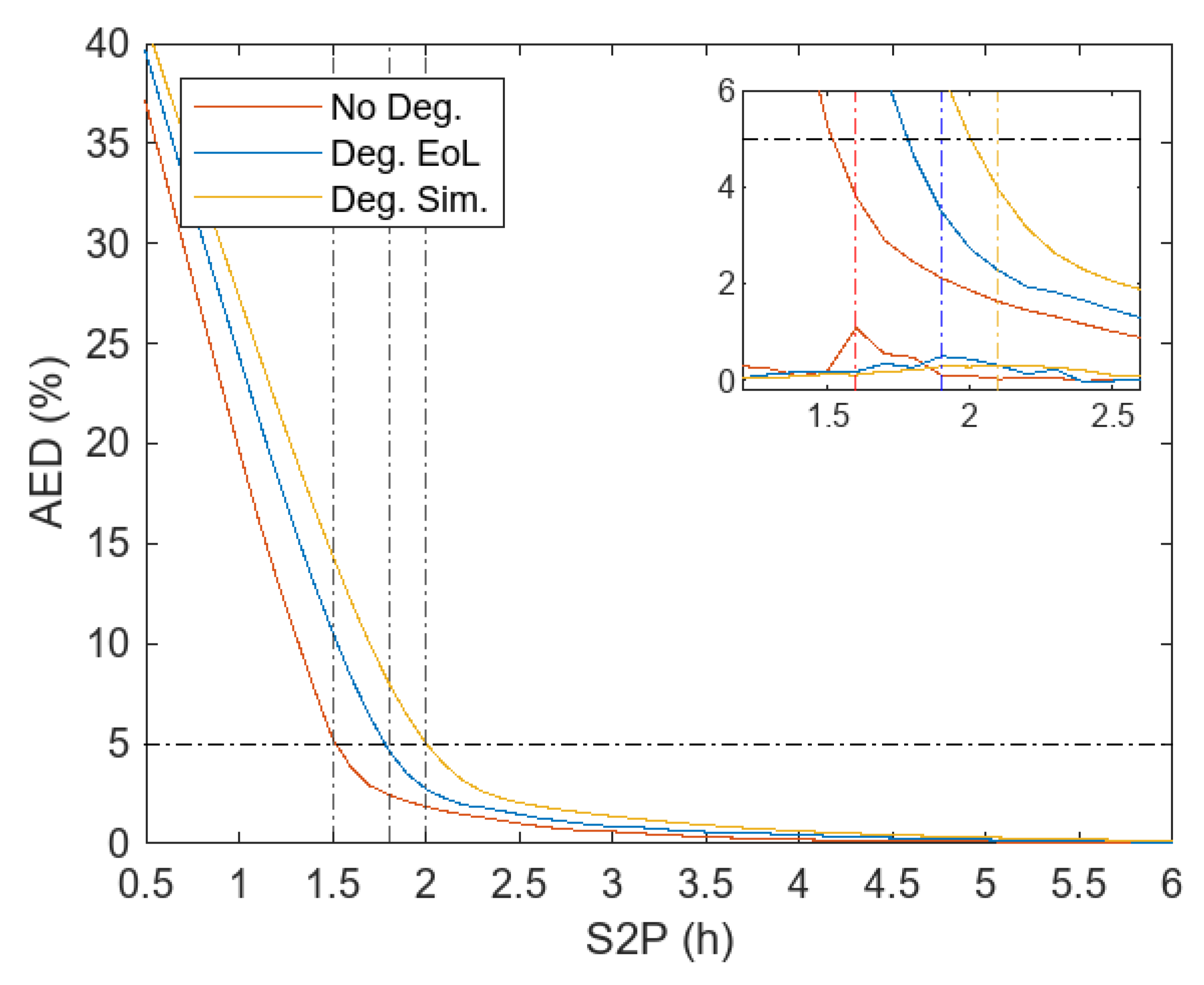
The curves in
Figure 15 show that there is a range of suitable storage sizes that guarantee the minimization of energy unavailability. The restriction is imposed that the AED indicator should not exceed 5%.
In order to examine the effect of degradation on the AED indicator, several scenarios have been presented in
Figure 15. The “No Deg.” curve, colored in red, simulates a hypothetical scenario in which the BESS operates without any degradation throughout its useful life until the End of Life. The “Deg. EoL” curve, represented in blue, reflects a more realistic scenario where the system experiences degradation until the End of Life.
The results obtained demonstrate that, to ensure an energy unavailability of less than 5%, a BESS with a capacity of S2P = 1.5 would be adequate in the theoretical scenario without degradation. However, when considering a realistic system of degradation in storage systems, it is necessary to increase the capacity to a value of S2P = 1.8 in order to reach the same threshold of energy unavailability. Consequently, it is significant that it is necessary to increase the storage capacity by 20% when taking into account the degradation phenomena in the BESS. This contrast underscores the importance of incorporating degradation factors in the design and sizing of BESSs.
It is commonly accepted to replace storage systems when they reach their EoL and the degradation reaches 20%. However, as the primary purpose of the PV-BESS is to ensure a constant power supply with low unavailability (AED < 5%), it is advisable to consider the possibility of slightly oversizing the BESS by extending its useful life. This oversizing, as illustrated in
Figure 13, involves increasing the S2P parameter and extends the time period until the EoL is reached. At the same time, this oversizing compensates for the gradual decrease in capacity due to degradation.
In
Figure 15, the blue curve, labeled “Deg. EoL”, shows how the AED rate behaves in a simulation until reaching the end of the BESS useful life of 44,352 h. On the other hand, the curve in yellow, called “Deg. Sim.”, represents the AED index for the complete simulation, which covers a total of 96,432 h.
Selecting a value of S2P = 1.8 is considered appropriate to ensure that unavailabilities are less than 5% until the BESS EoL is reached. However, as seen in
Figure 15, oversizing the BESS with a value of S2P = 2 ensures that the AED index remains below 5% throughout the simulation period, thus prolonging the useful life of batteries beyond the EoL. Specifically, this strategy extends the useful life from 44,352 h to a total of 96,432 h.
Additionally,
Figure 15 shows a saturation zone beyond which increases in storage capacity do not lead to substantial reductions in unavailability. Therefore, the choice of the S2P parameter must be made before reaching the saturation point to optimize the selected storage size.
For the particular case proposed in
Figure 15, the choice of S2P must be carried out in a way that guarantees that the unavailability (AED) remains below 5% at the end of the saturation elbow.
At the bottom of the zoom box in
Figure 15, the second derivatives of the curves are plotted to highlight possible significant changes in the trend. The second derivative provides details about the concavity of the function. Therefore, the S2P value is chosen at which the maximum of each of these derivatives is reached, since this indicates a change in the trend.
The choice of S2P is optimized to ensure that unavailability remains below 5%. For a simulation up to the EoL, a value of S2P = 1.9 is required. However, if you are looking to prolong the life of the batteries, you could consider selecting a value of S2P = 2.1, as long as no failures occur in the batteries, since beyond the EoL, the manufacturer does not guarantee its correct functioning.
This strategy of prolonging the useful life of the batteries is presented as an innovative and risky choice, although valid, in terms of achieving reduced unavailability while optimizing the size of the BESS.
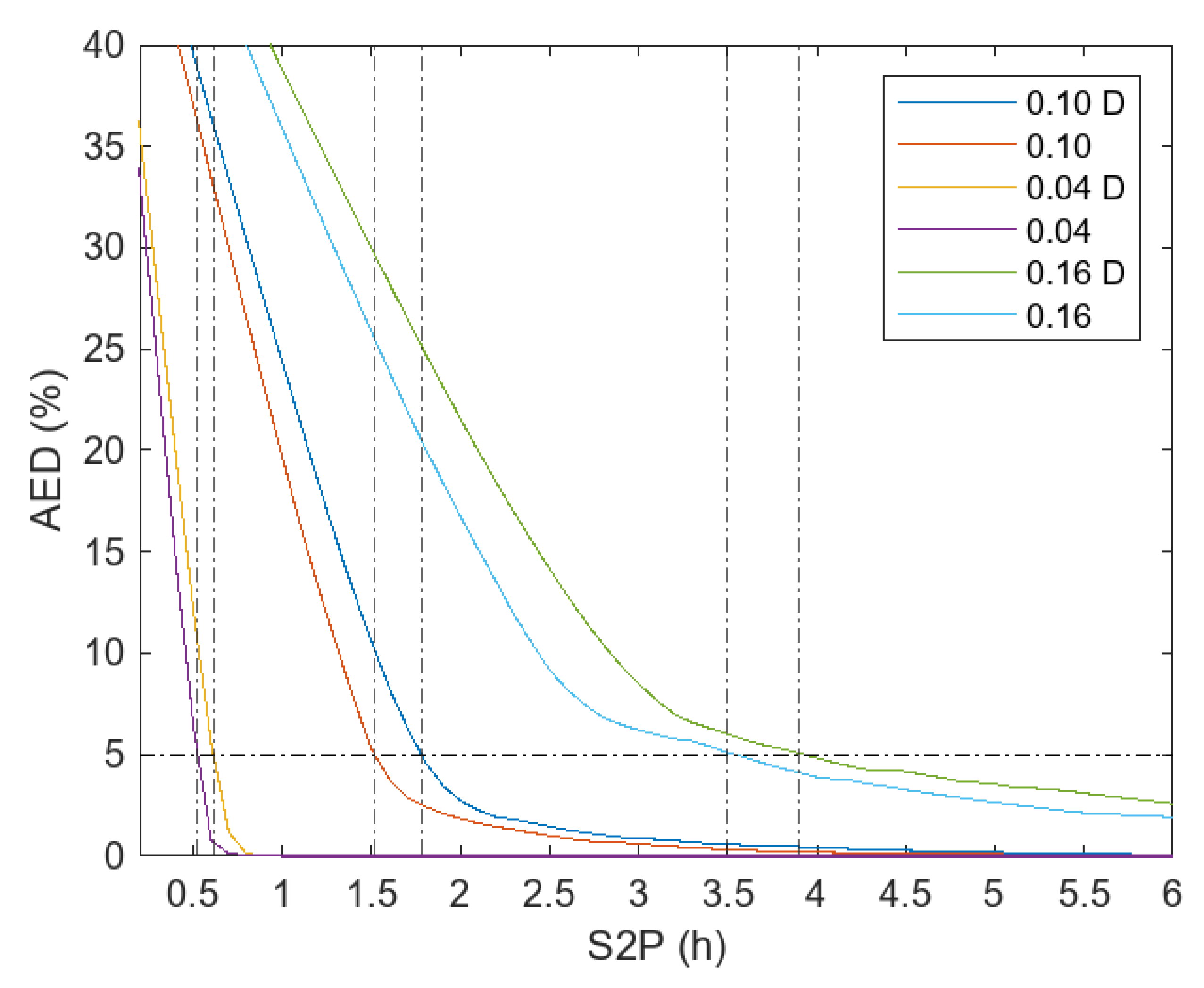
3.5. The Influence of the Power Setpoint on the Selection of the BESS with Degradation
In order to analyze the behavior of the AED indicator and determine the appropriate size of the BESS for different power setpoints, a comparison of three different scenarios is carried out. The first is a case of reduced power supply (CPOF = 0.04) to guarantee high energy availability for the system. The second is a case with a high power supply close to the maximum capacity factor that a PV plant can provide (CPOF = 0.16). The third case is the one proposed in the previous subsection (CPOF = 0.1) as a reference to compare results.
In
Figure 16, two different curves are presented for each scenario analyzed. One curve represents the theoretical situation without degradation effects, while the second incorporates the degradation effects proposed in this study. For ease of identification, the curve reflecting the degradation is labeled with the letter “D” in the legend of
Figure 16.
In order to guarantee that the PV-BESS complies with energy unavailability of less than 5% for a CPO
F of 0.04, it can be seen in
Figure 16 that the case without degradation requires an S2P = 0.5. However, when considering degradation phenomena, it is necessary to increase S2P to 0.62, which implies an increase in storage of 24%. For a CPO
F of 0.1, it is necessary to increase S2P from 1.5 to 1.8 when including degradation effects, which implies a 20% increase in S2P. For a CPO
F of 0.16, it is necessary to increase S2P from 3.5 to 3.85 by including the degradation of the BESS, which represents an increase of 10%.
Consequently, it is significant to highlight that as the power setpoint supplied by the system increases, the influence of degradation decreases. This implies that it is necessary to oversize the BESS less to meet the proposed energy availability objective.
4. Conclusions
The high cost of storage systems continues to be a gap in the academic literature when investigating PV-BESS hybrid plants operating with a constant power supply. However, the falling price of storage systems could make this configuration viable.
This study focuses on the energy aspect, using a realistic model that includes the detailed degradation effects of storage. Although this research focused on a specific case, the results can be extrapolated to any scenario with storage systems combined with photovoltaics.
Simulations have assessed the degradation of the BESS and its significant impact on storage capacity. This degradation has a direct impact on cycling operations. Comparing the proposed model with and without the degradation, it is found that it is necessary to increase the storage capacity by 20% to keep the energy unavailability indicator at the same level.
The analysis of the AED indicator in relation to S2P identifies the presence of a saturation bend, where increases in S2P do not significantly reduce the AED indicator. Therefore, the saturation bend together with the 5% limit on AED delimits a region in which to select the storage size, avoiding unnecessary oversizing.
It has also been observed that it is beneficial to oversize the BESS slightly. This not only prolongs its lifetime but also compensates for the reduction in capacity, which keeps the AED indicator at a low level. Specifically, for an intermediate power setpoint, it is concluded that selecting an S2P value of 2.1 instead of 1.9 extends battery life by almost twice as long.
The proposed model is adaptable and can be applied to other power generation technologies. Since the implemented algorithm performs hourly operations in a vectorial manner, it would be feasible to include an additional column vector in addition to the current PV production. Therefore, as a future line of work, all the simulations proposed in this article could be carried out using a combination of power generation technologies. Wind generation could be a suitable option to combine with PV generation due to their different generation patterns. Wind tends to produce more energy at night and on cloudy days, while solar tends to produce more energy in the middle of the day and under clear skies.


