
Steady- and Transient-State CFD Simulations of a Modified Barra–Costantini Solar System in Comparison with a Traditional Trombe–Michel Wall


Abstract
:1. Introduction
2. Materials and Methods
2.1. Steady State
2.2. Transient State
3. Numerical Methods
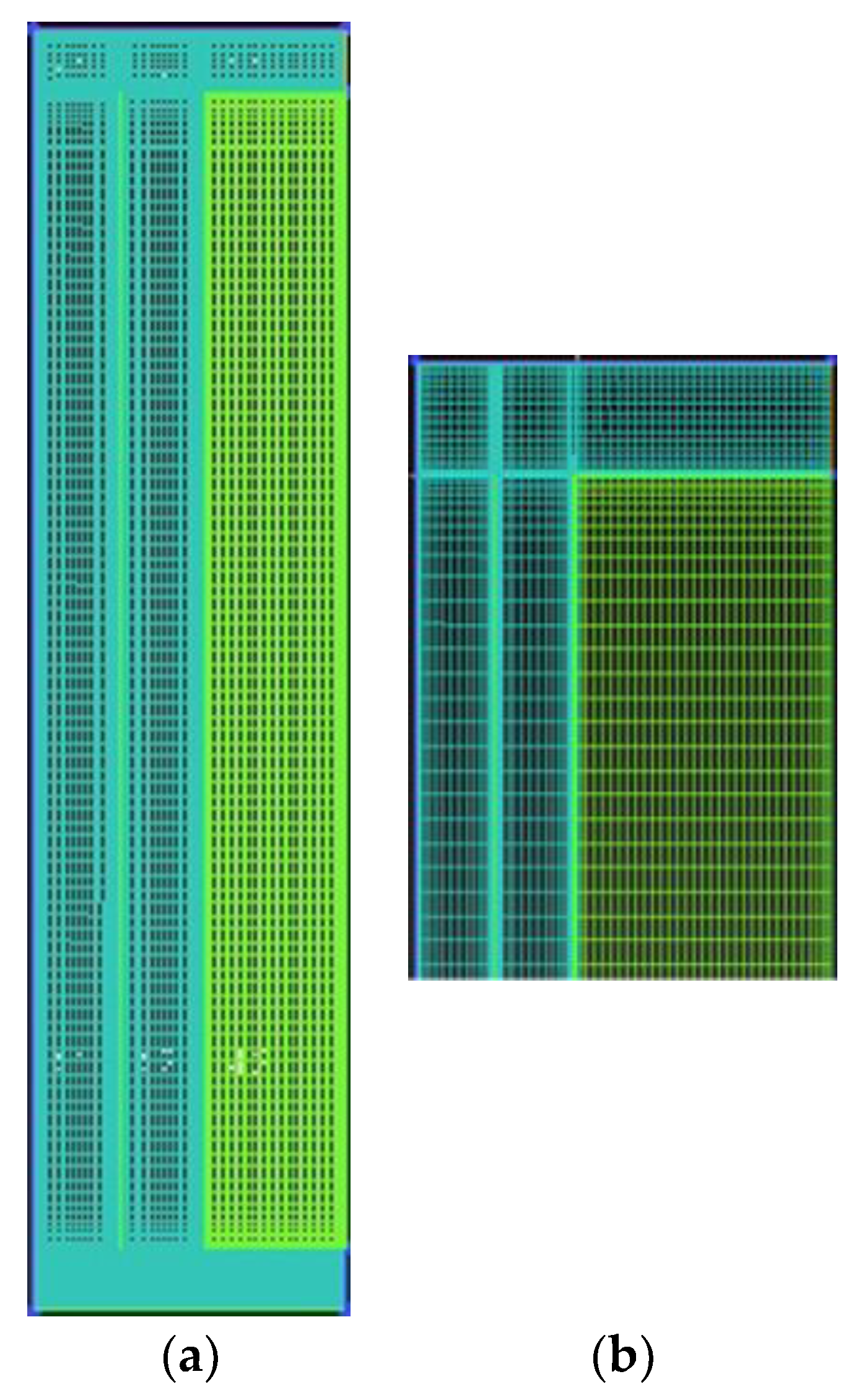
3.1. Computational Domain
3.2. Steady-State Simulations
3.3. Transient-State Simulations
4. Results
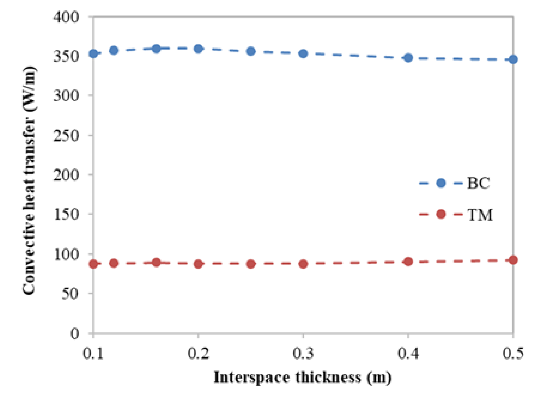
4.1. Steady State
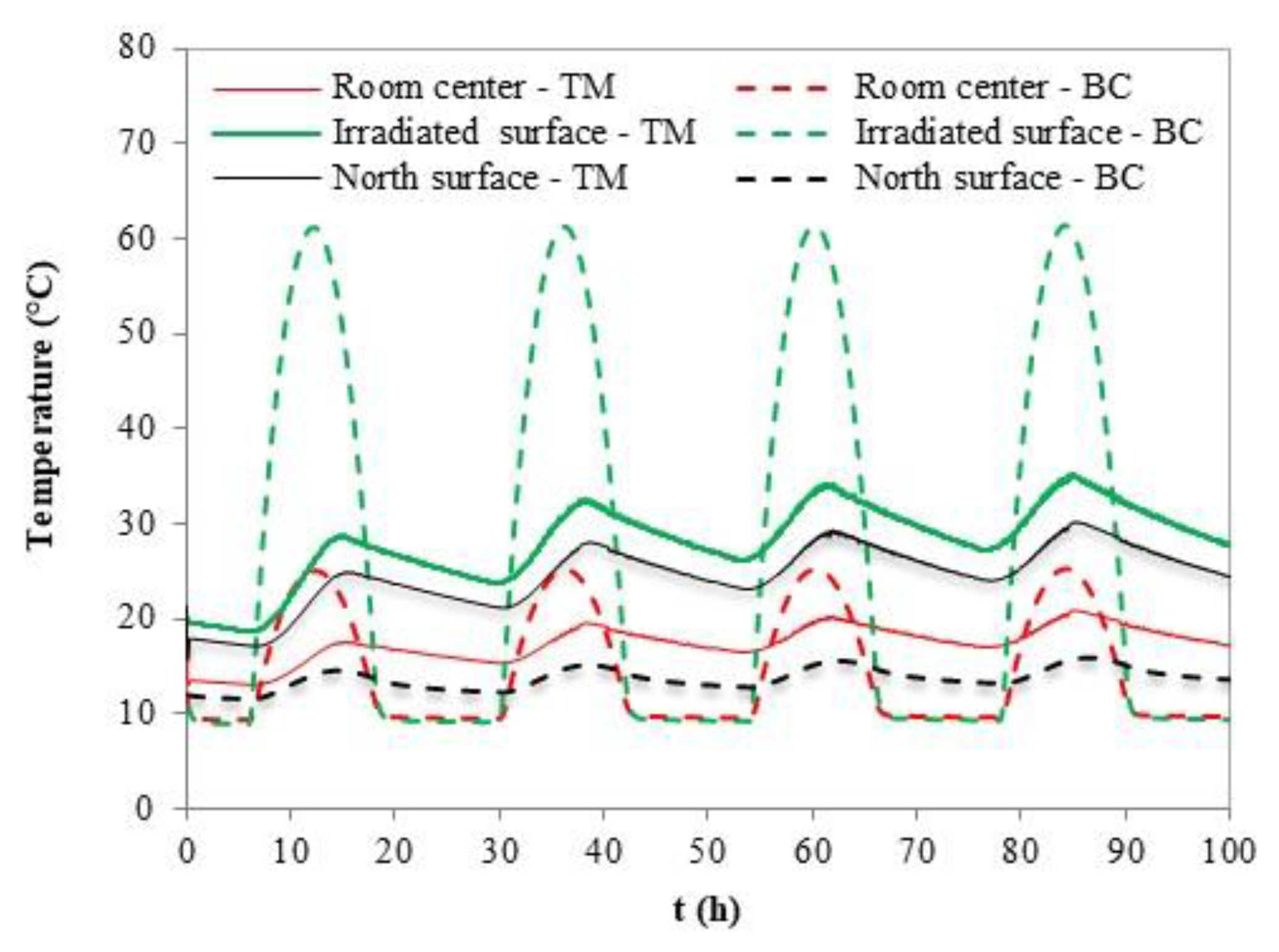
4.2. Transient Regime Results
5. Conclusions
Author Contributions
Funding
Data Availability Statement
Conflicts of Interest
Appendix A
Appendix A.1. Governing Equations
Appendix A.2. Turbulence Modeling
References
- Bellos, E.; Tzivanidis, C.; Zisopoulou, E.; Mitsopoulos, G.; Antonopoulos, K.A. An innovative Trombe wall as a passive heating system for a building in Athens—A comparison with the conventional Trombe wall and the insulated wall. Energy Build. 2016, 133, 754–769. [Google Scholar] [CrossRef]
- Perini, K.; Ottelé, M.; Fraaij, A.L.A.; Haas, E.M.; Raiteri, R. Vertical greening systems and the effect on air flow and temperature on the building envelope. Build. Environ. 2011, 46, 2287–2294. [Google Scholar] [CrossRef]
- Lichołai, L.; Starakiewicz, A.; Krasoń, J.; Miąsik, P. The Influence of Glazing on the Functioning of a Trombe Wall Containing a Phase Change Material. Energies 2021, 14, 5243. [Google Scholar] [CrossRef]
- Bruno, R.; Bevilacqua, P.; Cirone, D.; Perrella, S.; Rollo, A. A Calibration of the Solar Load Ratio Method to Determine the Heat Gain in PV-Trombe Walls. Energies 2022, 15, 328. [Google Scholar] [CrossRef]
- Abdullah, A.A.; Attulla, F.S.; Ahmed, O.K.; Algburi, S. Effect of cooling method on the performance of PV/Trombe wall: Experimental assessment. Therm. Sci. Eng. Prog. 2022, 30, 101273. [Google Scholar] [CrossRef]
- Jie, J.; Hua, Y.; Wei, H.; Gang, P.; Jianping, L.; Bin, J. Modeling of a novel Trombe wall with PV cells. Build. Environ. 2007, 42, 1544–1552. [Google Scholar] [CrossRef]
- Jie, J.; Hua, Y.; Gang, P.; Bin, J.; Wei, H. Study of PV-Trombe wall assisted with DC fan. Build. Environ. 2007, 42, 3529–3539. [Google Scholar] [CrossRef]
- Zhu, Y.; Zhang, T.; Ma, Q.; Fukuda, H. Thermal Performance and Optimizing of Composite Trombe Wall with Temperature-Controlled DC Fan in Winter. Sustainability 2022, 14, 3080. [Google Scholar] [CrossRef]
- Yilmaz, Z.; Kundakci, A.B. An approach for energy conscious renovation of residential buildings in Istanbul by Trombe wall system. Build. Environ. 2008, 43, 508–517. [Google Scholar] [CrossRef]
- Wang, X.; Xi, Q.; Ma, Q. A review of current work in research of Trombe walls. In Proceedings of the 2021 3rd International Conference on Civil Architecture and Energy Science (CAES 2021), Hangzhou, China, 19–21 March 2021; Volume 248, p. 03025. [Google Scholar] [CrossRef]
- Omara, A.A.M.; Abuelnuor, A.A.A. Trombe walls with phase change materials: A review. Energy Storage 2020, 2, e123. [Google Scholar] [CrossRef]
- Saadi, S.; Chaker, A.; Boubekri, M. Study of two new configurations of the Barra-Costantini system with sunspot modelling. Appl. Therm. Eng. 2020, 173, 115221. [Google Scholar] [CrossRef]
- Hong, X.; Leung, M.K.H.; He, W. Thermal behaviour of Trombe wall venetian blind in summer and transition seasons. Energy Procedia 2019, 158, 1059–1064. [Google Scholar] [CrossRef]
- Xiong, Q.; Alshehri, H.M.; Monfaredi, R.; Tayebi, T.; Majdoub, F.; Hajjar, A.; Delpisheh, M.; Izadi, M. Application of phase change material in improving Trombe wall efficiency: An up-to-date and comprehensive overview. Energy Build. 2022, 258, 111824. [Google Scholar] [CrossRef]
- Simoes, N.; Manaia, M.; Simoes, I. Energy performance of solar and Trombe walls in Mediterranean climates. Energy 2021, 234, 121197. [Google Scholar] [CrossRef]
- Wu, S.Y.; Yan, R.R.; Xiao, L. Numerically predicting the effect of fin on solar Trombe wall performance. Sustain. Energy Technol. Assess. 2022, 52, 102012. [Google Scholar] [CrossRef]
- Szyszka, J. Simulation of modified Trombe wall. In Proceedings of the SOLINA 2018—VII Conference SOLINA Sustainable Development: Architecture—Building Construction—Environmental Engineering and Protection Innovative Energy-Efficient Technologies—Utilization of Renewable Energy Sources, Solina, Poland, 19–23 June 2018; Volume 49, p. 00114. [Google Scholar] [CrossRef]
- Baxevanou, C.; Fidaros, D.; Tsangrassoulis, A. Analytical model for the simulation of Trombe wall operation with heat storage. Green Energy Sustain. 2021, 1, 0007. [Google Scholar] [CrossRef]
- Imessad, K.; Messaoudene, N.A.; Belhamel, M. Performances of the Barra–Costantini passive heating system under Algerian climate conditions. Renew. Energy 2004, 29, 357–367. [Google Scholar] [CrossRef]
- Zhang, L.; Dong, J.; Sun, S.; Chen, Z. Numerical simulation and sensitivity analysis on an improved Trombe wall. Sustain. Energy Technol. Assess. 2021, 43, 100941. [Google Scholar] [CrossRef]
- Corasaniti, S.; Manni, L.; Russo, F.; Gori, F. Numerical simulation of modified Trombe-Michel Walls with exergy and energy analysis. Int. Commun. Heat Mass Transf. 2017, 88, 269–276. [Google Scholar] [CrossRef]
- Hong, T.; Chou, S.K.; Bong, T.Y. Building simulation: An overview of developments and information sources. Build. Environ. 2000, 35, 347–361. [Google Scholar] [CrossRef]
- Albaqawy, G.; Mesloub, A.; Kolsi, L. CFD investigation of effect of nanofluids filled Trombe wall on 3D convective heat transfer. J. Cent. South Univ. 2021, 28, 3569–3579. [Google Scholar] [CrossRef]
- Hong, X.; He, W.; Hu, Z.; Wang, C.; Ji, J. Three-dimensional simulation on the thermal performance of a novel Trombe wall with venetian blind structure. Energy Build. 2015, 89, 32–38. [Google Scholar] [CrossRef]
- Long, J.; Jiang, M.; Lu, J.; Du, A. Vertical temperature distribution characteristics and adjustment methods of a Trombe wall. Build. Environ. 2019, 165, 106386. [Google Scholar] [CrossRef]
- Błotny, J.; Nems, M. Analysis of the Impact of the Construction of a Trombe Wall on the Thermal Comfort in a Building Located in Wrocław, Poland. Atmosphere 2019, 10, 761. [Google Scholar] [CrossRef]
- Zamora, B.; Kaiser, A.S. Thermal and dynamic optimization of the convective flow in Trombe Wall shaped channels by numerical investigation. Heat Mass Transf. 2009, 45, 1393–1407. [Google Scholar] [CrossRef]
- Koyunbaba, B.K.; Yilmaz, Z. The comparison of Trombe wall systems with single glass, double glass and PV panels. Renew. Energy 2012, 45, 111e118. [Google Scholar] [CrossRef]
- Hong, X.; Leungb, M.K.H.; He, W. Effective use of venetian blind in Trombe wall for solar space conditioning control. Appl. Energy 2019, 250, 452–460. [Google Scholar] [CrossRef]
- Hu, Z.; Wei He, W.; Hu, D.; Lv, S.L.; Jie, J.J.; Chen, H.; Ma, J. Design, construction and performance testing of a PV blind-integrated Trombe wall module. Appl. Energy 2017, 203, 643–656. [Google Scholar] [CrossRef]
- Yu, B.; He, W.; Li, N.; Zhou, F.; Shen, Z.; Chen, H.; Gang Xu, G. Experiments and kinetics of solar PCO for indoor air purification in PCO/TW system. Build. Environ. 2017, 115, 130e146. [Google Scholar] [CrossRef]
- Wang, D.; Hu, L.; Du, H.; Liu, Y.; Huang, J.; Xu, Y.; Liu, J. Classification, experimental assessment, modeling methods and evaluation metrics of Trombe walls. Renew. Sustain. Energy Rev. 2020, 124, 109772. [Google Scholar] [CrossRef]
- Bejan, A. Convection Heat Transfer; John Wiley and Sons: New York, NY, USA, 1984. [Google Scholar]
- Hussain AK, M.F.; Reynolds, W.C. The mechanics of an organized wave in turbulent shear flow. J. Fluid Mech. 1970, 41, 241–258. [Google Scholar] [CrossRef]
- Boussinesq, J. Essai sur la theorie des eaux courantes. Memoires presents par divers savants a l’. Acad. Des Sci. 1877, XXIII, 1–680. [Google Scholar]
- Menter, F.R. Two-equation eddy-viscosity turbulence models for engineering applications. AIAA J. 1994, 32, 1598–1605. [Google Scholar] [CrossRef]
- Wilcox, D.C. Reassessment of the scale-determining equation for advanced turbulence models. AIAA J. 1988, 26, 1299–1310. [Google Scholar] [CrossRef]


| Density kg/m3 | Thermal Conductivity W/(m K) | Specific Heat J/(kg K) | |
|---|---|---|---|
| Air | 1.225 | 0.0242 | 1006 |
| Aluminum absorber | 2719 | 202.4 | 871 |
| Concrete | 1800 | 1.6 | 880 |
| Hollow bricks | 850 | 0.251 | 1000 |
| Glass | 2500 | 0.8 | 670 |
Disclaimer/Publisher’s Note: The statements, opinions and data contained in all publications are solely those of the individual author(s) and contributor(s) and not of MDPI and/or the editor(s). MDPI and/or the editor(s) disclaim responsibility for any injury to people or property resulting from any ideas, methods, instructions or products referred to in the content. |
© 2024 by the authors. Licensee MDPI, Basel, Switzerland. This article is an open access article distributed under the terms and conditions of the Creative Commons Attribution (CC BY) license (https://creativecommons.org/licenses/by/4.0/).
Share and Cite
Corasaniti, S.; Manni, L.; Petracci, I.; Potenza, M. Steady- and Transient-State CFD Simulations of a Modified Barra–Costantini Solar System in Comparison with a Traditional Trombe–Michel Wall. Energies 2024, 17, 295. https://doi.org/10.3390/en17020295
Corasaniti S, Manni L, Petracci I, Potenza M. Steady- and Transient-State CFD Simulations of a Modified Barra–Costantini Solar System in Comparison with a Traditional Trombe–Michel Wall. Energies. 2024; 17(2):295. https://doi.org/10.3390/en17020295
Chicago/Turabian StyleCorasaniti, Sandra, Luca Manni, Ivano Petracci, and Michele Potenza. 2024. "Steady- and Transient-State CFD Simulations of a Modified Barra–Costantini Solar System in Comparison with a Traditional Trombe–Michel Wall" Energies 17, no. 2: 295. https://doi.org/10.3390/en17020295