Article

Wildfire-Induced Risk Assessment to Enable Resilient and Sustainable Electric Power Grid

1
Adlai E. Stevenson High School, Lincolnshire, IL 60069, USA
2
Lane Department of Computer Science and Electrical Engineering, West Virginia University, Morgantown, WV 26505, USA
*
Author to whom correspondence should be addressed.
Energies 2024, 17(2), 297; https://doi.org/10.3390/en17020297
Submission received: 16 November 2023 / Revised: 30 December 2023 / Accepted: 30 December 2023 / Published: 7 January 2024
(This article belongs to the Collection Renewable and Sustainable Energy)

Abstract

:
To ensure the sustainability of the future power grid, the rate of expansion of distributed energy resources (DERs) has introduced operational challenges. These include managing transmission constraints with DER power injection, dispatching DERs efficiently, managing system frequency, and ensuring sufficient reactive power for voltage support. Coupled with the intensification of wildfires, power infrastructures across the United States face challenges to minimize the impact of these factors and maintain system reliability and resiliency. This research embarked on a comprehensive evaluation, beginning with an in-depth historical analysis to delineate regions most susceptible to wildfires. Utilizing a multidimensional approach, the study assessed wildfire-induced risks to power grids by integrating historical wildfire occurrences, real-time wildfire proximities, Moderate-Resolution Imaging Spectroradiometer (MODIS)-derived vegetation metrics, and system parameters. Principal component analysis (PCA)-based optimal weights were then used, leading to the formulation of a novel risk factor model. This risk factor model has the potential to be the key to ensuring the resilience of a renewable-rich smart grid when faced with a severe weather event. Our model’s applicability was further verified through an empirical assessment, selecting representative networks from diverse regions, providing insights into the geographical variability of risk factors. Ultimately, this study offers stakeholders and policymakers a comprehensive toolset, empowering decisions regarding infrastructure investments, grid reinforcements, and strategic power rerouting to ensure consistent energy delivery during wildfires.

1. Introduction

The rapidly changing climate presents many complex challenges, with the relentless surge of wildfires carving an especially perilous niche. These wildfires, fed and intensified by climate anomalies, are detrimental to electric power systems. Wildfires are no longer just natural calamities; they have transformed into multifaceted disasters impinging upon both the natural environment and human-made infrastructure. The alarming consequences of wildfires for power systems cannot be understated. Components of power infrastructure, when exposed to such extreme events, can suffer irreparable damage, culminating in extensive power outages. Often, the ignition source for these wildfires is transmission and distribution infrastructure [1]. These blackouts, in turn, cause monumental economic losses and, paradoxically, can even become the birthplaces for more fires, perpetuating a vicious cycle [2]. In the United States, losses from the fires of 2020 in California are estimated at a record USD 19 billion [3]. The significant economic costs associated with these events come not just from direct damage but also from the subsequent ramifications in critical systems like the electric grid [4].
Although wildfires may be triggered naturally (most commonly by lightning), about ninety percent of them are caused by human activities like discarded burning cigarettes; unattended campfires; electrical equipment (faults in power lines, the failure of old electrical equipment, or the explosion of oil-filled power system apparatus); overheating automobiles, or arson [1,5]. High-velocity winds, which often accompany wildfires, can cause power conductors to sway violently, leading to contact with nearby trees or other flammable entities. Such contact has the potential to cause new, often more devastating fires, further aggravating the situation [6]. In their daily operations, electric utility providers can implement fewer and more disruptive actions to reduce the impacts of wildfires on the power grid. The most commonly used method is public safety power shut-offs (PSPSs) [7,8,9], where certain sections of the grid are de-energized, causing intentional blackouts. This significantly impacts both customers and the ability of the power system to provide reliable electricity. In October 2019, the intentional blackouts due to PSPSs affected almost a million customers [10].

2. Problem Statement

Confronted with such grim scenarios, the logical recourse might seem to be reinforcing the entire grid system, rendering it impervious to the threats posed by wildfires. However, this approach is fraught with complications. Primarily, the financial implications are enormous. A testament to this is PG&E’s estimation, which suggests that a budget exceeding USD 100 billion would be necessary to subterraneously route its high-voltage lines across two-thirds of California [11]. Moreover, this task is not without its environmental quandaries. Undertaking such massive underground operations in ecologically rich zones could lead to unforeseen environmental consequences. Recent history also provides testimony as to the vulnerability of the power infrastructure. The 2017 Thomas Fire serves as a stark reminder, having disrupted power transmission in the Santa Barbara region, leaving a staggering 85,000 customers in darkness. Fast forward a year, and the narrative remained equally bleak, with the Mendocino Complex Fire depriving approximately 50,000 residents of power. Northern California was not spared either. The mere threat of wildfires coerced utility companies into cutting off power for nearly 800,000 customers, underscoring the gravity of the situation [12]. Statistical trends only add to the concerns. On average, wildfires have impacted over 933,547 customers. A comprehensive study spanning 16 years revealed that damage to power transmission and distribution networks exceeded USD 700 million, a figure that is only expected to rise considering the escalating frequency and severity of wildfires, especially in regions like California [13].
With the resilience and reliability of the electrical infrastructure being put to the test, particularly by challenges emanating from natural disasters like wildfires, researchers have been tirelessly working to develop sustainable models for wildfire disruption mitigation. The authors of [14] proposed a new optimization model to minimize wildfire risk due to electric power system components while maintaining the electricity supply to as many customers as possible by considering how preventive wildfire risk measures impact both wildfire risk and power system reliability in a short-term, operational time frame. In [15], the authors proposed an optimization approach for the expansion planning of a power system considering the presence of High-Fire-Threat District (HFTD) zones, while ensuring the operational feasibility of the network. An optimal scheduling framework for managing power-system-induced wildfire risk was proposed in [16] and demonstrated over multiple time steps so that the risk of wildfire and load delivery fluctuation with changes in temperature and power demand throughout the day could be accounted for. The authors of [17] underscored the heightened risk that wildfires pose to electric power grids, in terms of both damage to electrical equipment and the safety of personnel. The authors of [18] proposed a Markov decision-process-based system state transition model to provide generation redispatch strategies for each possible system state given component failure probabilities, wildfire spatiotemporal properties, and load variation, in order to enhance the operational resilience of power grids during wildfires.
With the increased penetration of distributed energy resources (DERs) (which introduce stochasticity owing to their intermittency) both at the transmission and distribution levels, coupled with the increasing number of wildfires, the resiliency of the current power grids has been significantly impacted. Moreover, renewable energy resources or inverter-based resources (IBRs) do not provide power systems with enough inertia, which is the capacity of a power system to resist changes in frequency. The high penetration of IBRs increases the rate of change of the frequency (ROCOF), decreasing the inertia of power networks substantially. This can jeopardize the frequency stability in power systems, which is more problematic during the recovery process after an extreme event like a wildfire. Based on real-world data, [19] deduced that wildfires reduce solar generation, increase solar forecast errors, heighten day-ahead reserve requirements and real-time operating reserve shortages, and raise market prices. Wildfire smoke causes wiggling in the PV power output, which has the potential to impact the frequency stability of the grid [20]. A resilience enhancement strategy for severe weather events was developed in [21] to optimally coordinate wind farms with battery energy storage systems (BESSs), while [22] introduced a data-driven transmission hardening method to estimate the uncertainty sets associated with DERs. However, both of these methods were devised for the planning phase and might not consider the variabilities faced by the system during operation.
Recognizing that fortifying the entire grid is neither financially nor environmentally viable, and PSPSs are not a viable option for grid reliability, we endeavored to provide a nuanced solution. By meticulously analyzing vulnerabilities, this study aimed to equip policymakers with the intelligence to prioritize regions that are most at risk, thereby ensuring that reinforcement efforts are both strategic and effective. The objective of this work was to develop a proactive risk assessment approach for power grid wildfire susceptibility. The key contributions include:
  • We developed an architecture and algorithms for predictive analysis to identify power grid nodes at heightened risk even before wildfire events unfold. This algorithm utilizes environmental parameters, historical wildfire occurrences, vegetation types, and voltage data for predictive analysis.
  • We developed a region-specific risk analysis approach for wildfires using principal component analysis (PCA), isolating the most influential determinants of node vulnerability. The developed algorithm employs Moderate-Resolution Imaging Spectroradiometer (MODIS)-derived vegetation metrics, Hierarchical Density-Based Spatial Clustering of Applications with Noise (HDBSCAN), Voronoi-HDBSCAN, and enhanced proximity analysis using an overlay of the electric grid and wildfire coordinates. Furthermore, by undertaking a comparative analysis across five distinct regions, our research elucidates region-specific risk profiles, paving the way for tailored future mitigation strategies.
In our work, a node represents a large-scale geographical region overlayed by electric nodes within a regional area. Fast-response DERs can be utilized to provide generation when the dynamically calculated risk factors cross a pre-determined threshold, indicating a potential loss of heavily loaded lines, in order to ensure a reliable power supply to customers while reducing loading at the high-risk nodes, which in turn will reduce their risk factors. Researchers from LBNL [23] studied the factors impacting the resilience of critical infrastructure such as hospitals and data centers and developed the Distributed Energy Resources Customer Adoption Model (DERCAM) to optimize the configuration of DER-based microgrids to support single- and multi-day outages. Researchers have also explored optimal long-term resilient expansion planning strategies, offering utilities providers three types of network expansion decisions ((1) the addition of new lines; (2) the modification of existing lines; and (3) the installation of distributed energy resources (DERs), specifically renewable resources) with a two-stage robust optimization problem to ensure power system resilience against unfavorable events [24]. In [25], model predictive control was implemented to adjust the system topology as well as the DER operation set points based on updated fault information and DER forecasts, in order to dynamically enhance system resilience against extreme weather events. Our work provides a predictive analysis to help with such post-detection mitigation frameworks and enhance grid resilience through anticipatory intelligence.

3. Analysis of Historical Wildfire Data

With the increased penetration of renewable generation across the grid, system operators have the onerous task of maintaining the fragile balance of power consumption and generation while ensuring system stability. Along with reducing system inertia, renewable generation brings a certain level of uncertainty into the equation. As a result, during severe weather events such as wildfires, when several components of the grid are impacted simultaneously, maintaining stability in the rest of the network becomes a challenge. To ensure the resilience of the power network, we need to understand the behavior of wildfires. To this end, we used available historical data on various wildfires across the nation as a starting point.
Understanding the likelihood of forest fires occurring in a region should be the first step in developing a reliable risk assessment model. Using the wildfire events as data points, Figure 1 illustrates the construction of a density-based spanning tree (DBST), which offers a robust framework for understanding and identifying clusters in a hierarchical, density-based manner. Through mutual reachability distances and persistence measures, Hierarchical Density-Based Spatial Clustering of Applications with Noise (HDBSCAN) provides a nuanced yet computationally efficient approach to clustering large datasets.

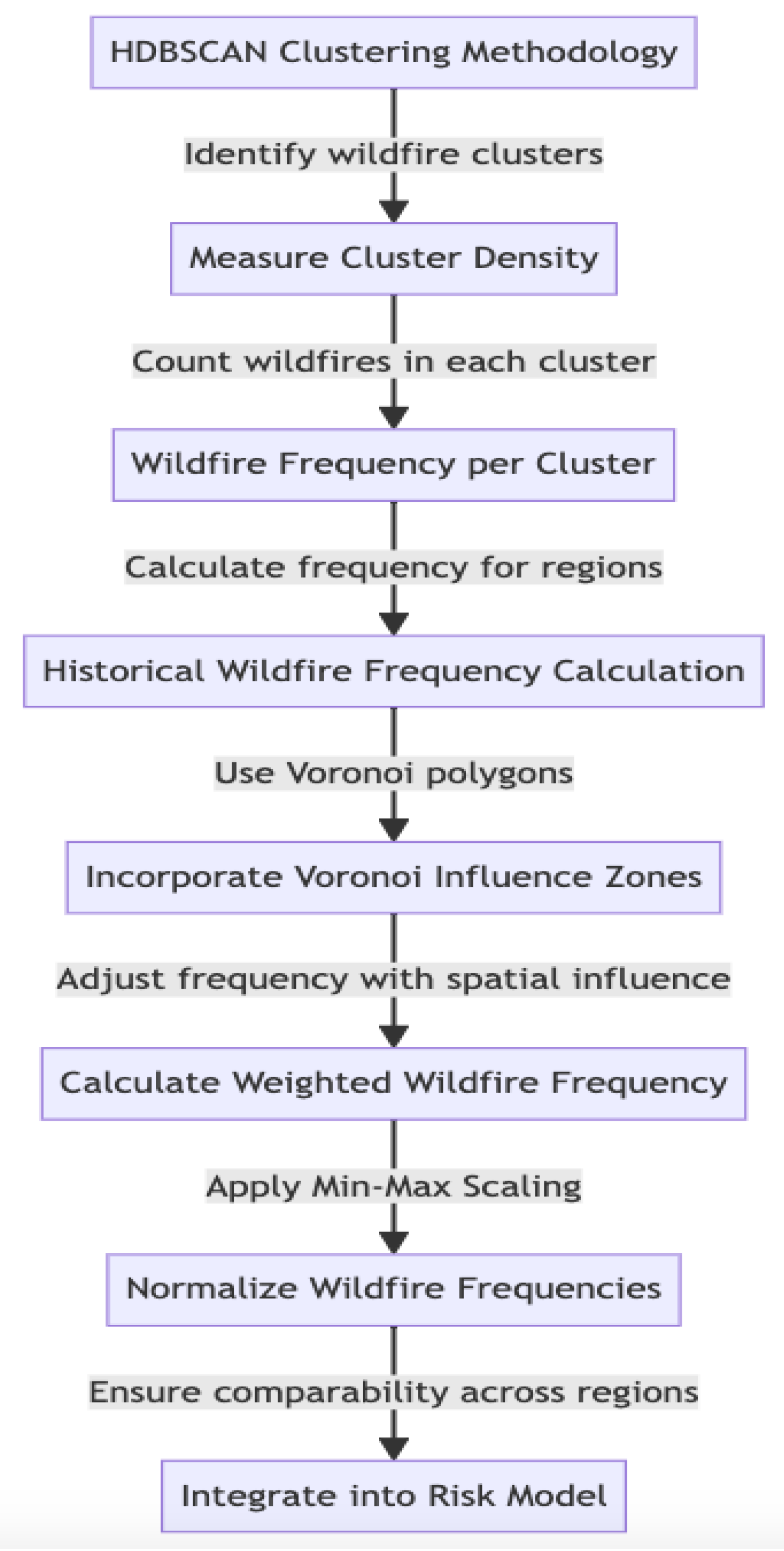
3.1. Density-Based Spatial Clustering: HDBSCAN

Hierarchical Density-Based Spatial Clustering of Applications with Noise (HDBSCAN) is an offshoot of the DBSCAN algorithm. Unlike K-means, which requires the pre-specification of clusters, HDBSCAN, with its foundation in density, provides a more fluid understanding of clusters. Given a set X = { x 1 , x 2 , , x n } , the algorithm calculates the core distance and the mutual reachability distance. For any point x, its core distance, d c o r e ( x ) , is the smallest radius such that there exists at least M i n P t s in its neighborhood:
d c o r e ( x ) = radius such that | N M i n P t s ( x ) | M i n P t s
where | N M i n P t s ( x ) | denotes the number of points within that radius. To formalize this, let us assume that we have a dataset D with n data points. For any two points p , q in D, the mutual reachability distance is defined as
mutual _ reach _ dist ( p , q ) = max { core _ dist ( p ) , core _ dist ( q ) , d ( p , q ) }
were:
  • d ( p , q ) is the usual distance metric, e.g., Euclidean distance.
  • core _ dist ( p ) is the distance from point p to the M i n P t s th nearest point in D.
This mutual reachability distance ensures that distant points in dense regions are not over-penalized. Using these distances, a minimum spanning tree (MST) is created, where nodes represent data points, and edges represent the mutual reachability distances between them.
The MST is then found using Kruskal’s algorithm [27], which operates efficiently with a time complexity of O ( n 2 log n ) . Within the MST, the order in which the edges are considered gives insight into the hierarchical structure of the data:
  • Edges with the smallest mutual reachability distance (indicating high density) are considered first.
  • As we traverse edges with increasing distances, we transition from denser to sparser regions, hierarchically branching the data.
This hierarchy represents the density-based structure of the data, where each level corresponds to a varying density threshold.
The final step, pruning, is carried out based on a persistence measure. The persistence of a cluster is the difference between its birth (when it first appears) and death (when it merges into another cluster) in terms of the mutual reachability distance. A higher persistence indicates a more stable and distinct cluster. By setting a threshold for persistence, branches (clusters) with low persistence (unstable over the range) are pruned, and the remaining branches are identified as the final clusters.

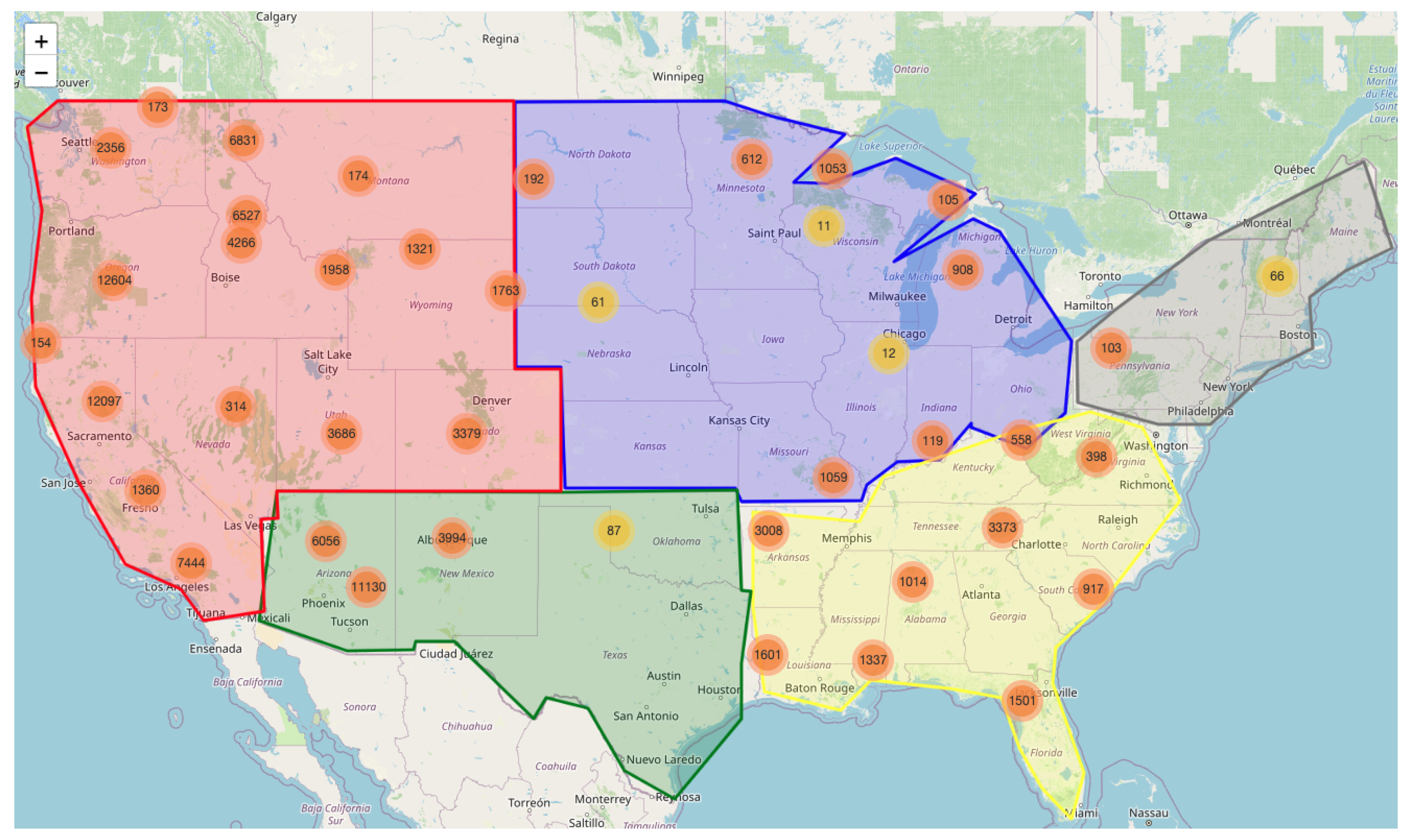
3.2. Regional Analysis with Voronoi-HDBSCAN

Introducing polygons, especially when analyzing regions, can provide contextual understanding. We used Voronoi polygons to visually represent the influence zone of each data point (wildfire event).
Given a set of points P in the plane, a Voronoi diagram divides the plane such that every point within a particular region is closer to the seed point of that region than any other. Mathematically, for a seed point p i in P, its Voronoi region V ( p i ) is
V ( p i ) = { x R 2 : d ( x , p i ) < d ( x , p j ) j i }
where d is the distance measure, typically Euclidean.
Combining Voronoi diagrams with HDBSCAN clusters allows us to visualize not just where clusters are but also the influence area of each cluster’s members. For each of the five main regions of the US, Voronoi diagrams were superimposed on the HDBSCAN clusters. The susceptibility S r for each region was adjusted as follows:
S r = A r e a ( V H r ) A r e a ( H r ) × 100
where V represents the union of Voronoi regions associated with wildfire events, and H r represents the total area of region r.
It is evident from Figure 2 that the West and Southwest regions of the US showed heightened susceptibility values. The Voronoi-HDBSCAN method reveals critical insights into how wildfires are distributed and their regional influence, a novel approach beneficial for strategic planning.

4. Novel Wildfire Risk Factor Components

Contemporary electrical grids, with their sprawling network of transmission lines and buses, encounter multifaceted environmental challenges that necessitate sophisticated analytical approaches. One of the emergent challenges is the proximity of wildfires to critical grid infrastructure. The dynamics of these wildfires, which are both temporal and spatial, require the seamless integration of real-time monitoring and robust mathematical models to ascertain potential risks to the grid, as illustrated in Figure 3.

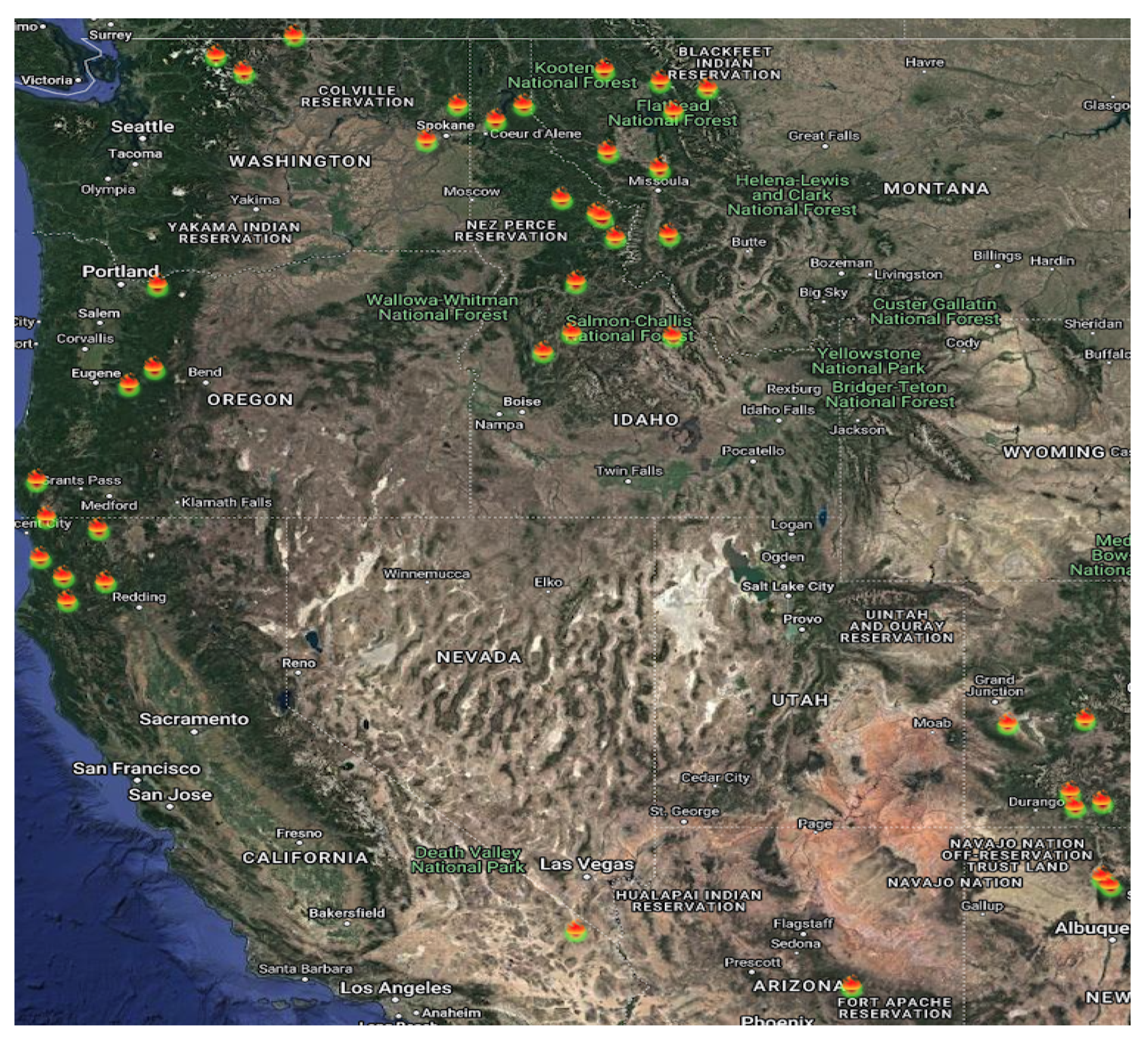
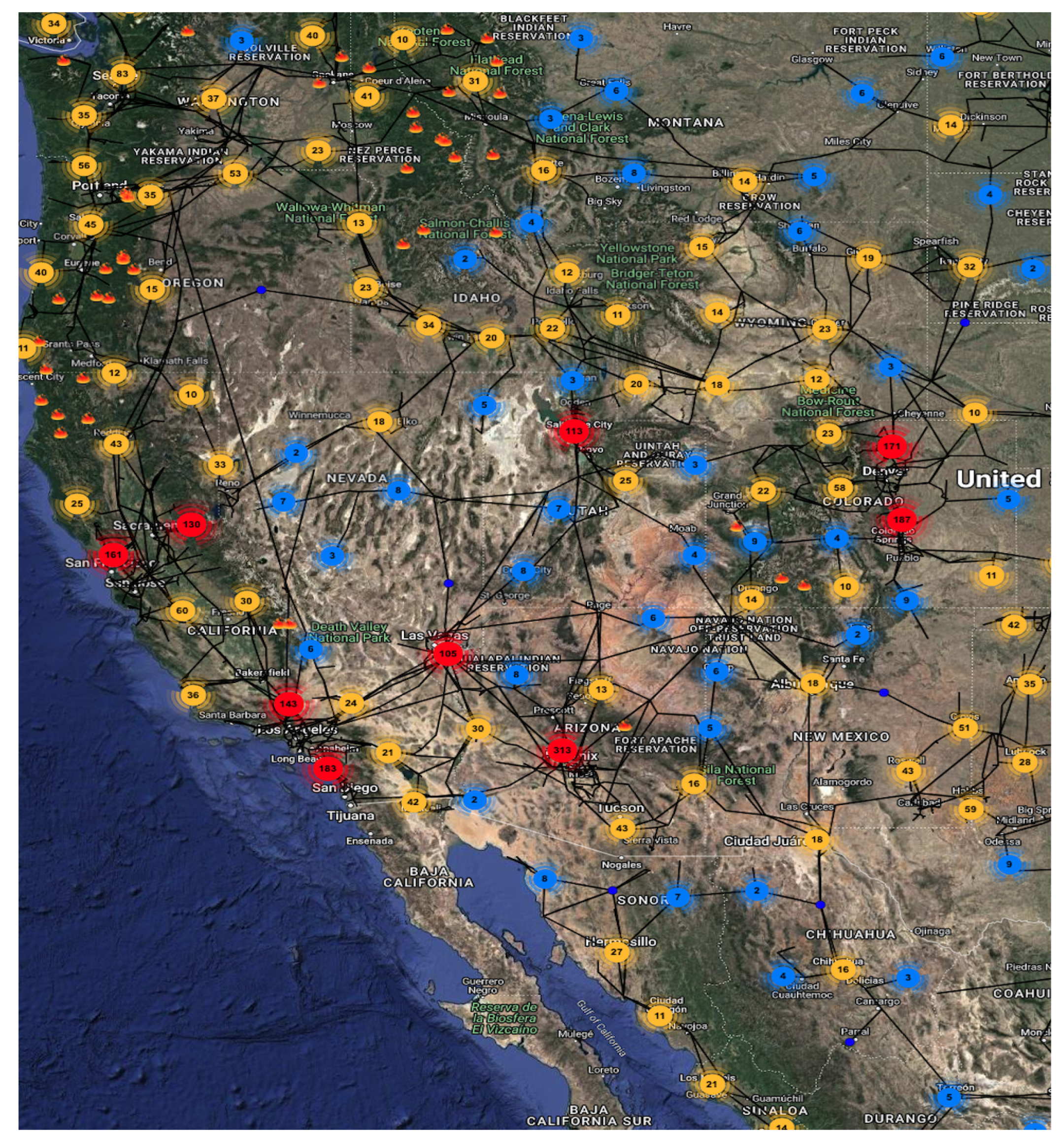
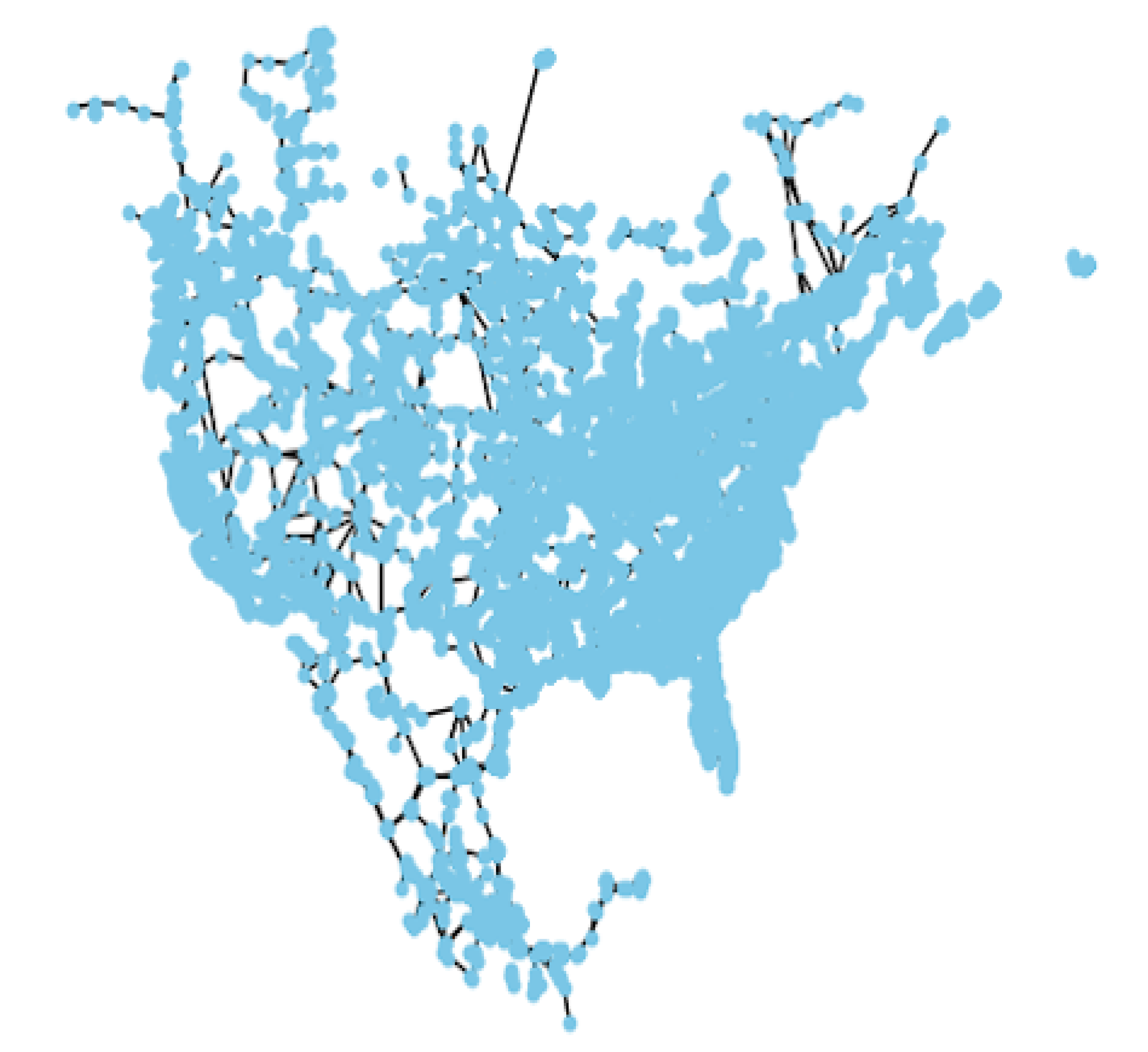
4.1. Enhanced Proximity Analysis between Wildfire Incidents and Electrical Grid

While there are multiple methods to determine the distance between two geographical points, the Haversine formula stands out for its accuracy, especially for significant spans on a spherical body like Earth. This formula, rooted in trigonometric principles, precisely calculates the great-circle distance, which is the shortest distance between any two points on the surface of a sphere. For two geocoordinates P 1 ( λ 1 , ϕ 1 ) and P 2 ( λ 2 , ϕ 2 ) ,
Δ ϕ = ϕ 2 ϕ 1 Δ λ = λ 2 λ 1 a = sin 2 Δ ϕ 2 + cos ( ϕ 1 ) × cos ( ϕ 2 ) × sin 2 Δ λ 2 c = 2 × asin a d = R × c
where R is the Earth’s radius, and d is the computed distance.
In the project’s schema, the electrical grid is represented by a graph G ( V , E ) , with V and E being sets of nodes (buses) and edges (transmission lines), respectively. The vulnerability or risk factor of a node, r v , is influenced by various parameters, with the proximity to active wildfire regions, calculated using the Haversine formula, being a principal factor. This is denoted as d ( v , W ) for a node v and wildfire location W. Specifically,
r v = f ( d ( v , W ) , P )
where, f is a risk determination function, and P represents other parameters influencing risk, such as meteorological conditions, grid load, and infrastructure age.
The application protocol can be articulated as follows:
  • Extract the real-time geocoordinates of active wildfire incidents.
  • For each node v V , utilize the Haversine formula to compute d ( v , W ) .
  • Integrate d ( v , W ) into the risk function f to update the risk factor r v for each node.
  • Prioritize nodes based on increasing risk values, thereby aiding in real-time grid management decisions.
A critical aspect of risk evaluation in the context of proximity analysis is the normalization of derived distances. While the Haversine formula provides an accurate measure of the great-circle distance between two geographical points, these absolute values may span a vast range. For a uniform and comparative risk assessment, it is essential to map these distances to a normalized scale, typically between 0 and 1.
One of the most common normalization methods is min-max scaling. Given a distance d ( v , W ) and assuming d max and d min are the maximum and minimum distances observed across all nodes, respectively, the normalized distance d norm ( v , W ) can be computed as
d norm ( v , W ) = d ( v , W ) d min d max d min
However, in the context of risk, proximity to a wildfire poses a higher threat. Thus, it might be more intuitive to invert this normalized value, with a value closer to 1 indicating closer proximity and, therefore, a higher risk:
d norm ( v , W ) = 1 d norm ( v , W )
Incorporating this normalized distance measure into the risk determination function ensures that the proximity influence is consistent across all nodes, regardless of their absolute geographical separations. Moreover, this allows for a clear comparison among nodes, where nodes with values closer to 1 are in more immediate danger and might require urgent interventions.
The Haversine formula provides a rigorous mathematical foundation for the proximity-based risk analysis of the electrical grid in relation to wildfire threats. Figure 4 implements this by displaying the visualization of how the Haversine Formula is used with regards to real-time wildfires and individual substations. This, when combined with other risk parameters, offers a holistic and highly accurate risk assessment model, which is essential for the safeguarding and efficient management of contemporary electrical grids.

4.2. Historical Wildfire Frequency as a Risk Factor

The spatial distribution of wildfires across different regions bears testament to not only environmental conditions but also human activities, forest management practices, and various socio-economic factors. However, for the sake of electrical grid robustness, it is paramount to convert these spatial patterns into quantifiable metrics that can be used as risk indicators. Historical wildfire frequency emerges as a pivotal metric in this scenario.
Using the HDBSCAN clustering methodology, clusters of historical wildfires are identified across regions. Each cluster’s density provides an immediate measure of wildfire frequency for that specific region. Let us denote the number of wildfires in a given cluster C i as W ( C i ) .
To determine the historical wildfire frequency F r for a region r, the following equation can be employed:
F r = i C l u s t e r s r W ( C i ) A r e a ( H r )
where C l u s t e r s r are the identified clusters in region r, and A r e a ( H r ) is the total area of region r.
To incorporate the influence zones identified through Voronoi polygons, a weighted frequency can be used. This takes into account not just the number of wildfire events but also their spatial influence:
W F r = i C l u s t e r s r W ( C i ) × A r e a ( V H r ) A r e a ( H r )
where A r e a ( V H r ) represents the union of Voronoi regions associated with wildfire events in region r. This weighted wildfire frequency, W F r , provides a more nuanced understanding of the historical wildfire frequency by integrating spatial influence areas.
Given the vast differences in regional sizes and historical data availability, it is essential to normalize these frequency values. Again, min-max scaling is used, where the minimum is 0 and the maximum is 1:
N F r = W F r min ( W F ) max ( W F ) min ( W F )
Here, N F r is the normalized frequency for region r, and min ( W F ) and max ( W F ) are the minimum and maximum weighted frequencies among all regions, respectively. This normalized metric ensures comparability across regions irrespective of their size and can be directly integrated as a factor in the risk model.
The historical wildfire frequency, especially when weighted by spatial influence, provides an invaluable insight into the regions more likely to experience future events. It is grounded in the notion that past events indicate areas of inherent vulnerability, whether due to local environmental conditions or human factors. By incorporating the process illustrated by Figure 5 into the risk model, the electrical grid’s representation and analysis become more in line with real-world challenges, making it a vital component in assessing potential future vulnerabilities.

4.3. Voltage Analysis in Electrical Grid Nodes and Transmission Lines

Voltage, in power systems, is not merely an electrical parameter but a crucial indicator of the system’s health, stability, and operational efficiency. The magnitude and phase of voltage across nodes (buses) and transmission lines can shed light on a plethora of system attributes, from load dynamics to reactive power compensation.
As shown in Figure 6, the granular voltage information for each node and transmission line within our framework was acquired from a comprehensive dataset, meticulously curated from multiple sensors and telemetry equipment distributed across the grid. These sensors, often connected to sophisticated Supervisory Control and Data Acquisition (SCADA) systems, provide near-real-time measurements.
Let us first denote the voltage at any node i as V i , which can be expressed in polar form as
V i = | V i | θ i
In power systems, the power flow equation that relates voltage and power is
P i + j Q i = k = 1 n | V i | | V k | Y i k ( θ i k θ i + θ k )
For transmission lines, the voltage drop can be represented using the line impedance Z = R + j X :
Δ V = I l i n e × Z
Voltage data for the nodes and across transmission lines are dynamically linked within our advanced grid management framework. For any node i, the voltage profile over time t can be formulated as
V i ( t ) = V b a s e + 0 t Δ V i ( τ ) d τ
Operational state of a node or transmission line is influenced by its voltage magnitude. The evaluation of the eigenvalues of the system’s Jacobian matrix is conducted as follows:
J = P / θ P / | V | Q / θ Q / | V |
Voltage deviations, both sag (when demand is higher than generation) and swell (when generation is higher than demand) [30], can indicate potential grid vulnerabilities. The normalization of voltage magnitudes ensures that the operational state of each node can be compared, offering a unified measure of vulnerability.
Given a node’s voltage magnitude | V i | and taking into account the permissible voltage range [ V min , V max ] specified by grid standards, the normalized voltage magnitude V norm , i can be computed using min-max normalization.
However, from a risk perspective, significant deviations from the nominal voltage value (either too high or too low) are more concerning. Thus, it might be valuable to use a modified normalization scheme that accentuates deviations:
V norm , i = 1 V norm , i 0.5 × 2
Here, V norm , i inverts the normalized voltage such that values approaching 0 indicate nominal operation, and as the voltage deviates from nominal (either due to sag or swell), V norm , i increases, approaching 1. This renders nodes with a V norm , i value closer to 1 as more vulnerable, warranting monitoring or corrective action.
This normalization approach ensures that voltage magnitudes, irrespective of their absolute value, contribute consistently to the risk assessment metric. By centering the scale on nominal operational values and expanding outward to encompass extreme vulnerabilities, grid operators and analysts can prioritize nodes based on their deviation from desired operational standards.
It is worth noting that while this normalization provides a framework for assessing vulnerability, a comprehensive risk assessment might necessitate further refinements considering other voltage-related parameters like voltage stability margins, phase imbalances, and harmonic distortions. By integrating real-time voltage data and coupling them with mathematical models, our framework offers insights into the operational health of the grid.

4.4. Vegetation-Based Wildfire Risk Assessment using MODIS Data

The first step in the process involves retrieving vegetation data from the MODIS API provided by NASA. The primary metric to be extracted is the NDVI (Normalized Difference Vegetation Index), which provides insight into the density and health of vegetation in a given area. This is given by
NDVI = ( NIR Red ) ( NIR + Red )
Here, NIR stands for the near-infrared reflectance, and Red stands for the red light reflectance. Using the NDVI values, areas can be classified into different types of vegetation. The classification process is based on established NDVI ranges that correspond to the given vegetation categories. For instance, specific NDVI value ranges can indicate grassland, while others can signify dense forests.
After classifying vegetation, it is essential to understand the characteristics of each vegetation type. For each category, parameters such as fuel loading, fuel bed depth, surface area to volume ratio, and packing ratio are analyzed [31]. These detailed data often serve as one of the factors for wildfire risk assessment, giving insight into how easily a fire can ignite and spread, and how intense it might become.
Once we have detailed vegetation parameters, we can quantify the wildfire risk for each individual node. The wildfire risk for each node in relation to the vegetation type is then quantified using the derived function:
R node = region F ( Fuel Loading ( x ) , Fuel Bed Depth ( x ) , Packing Ratio ( x ) , ) d x
This function encapsulates the cumulative risk based on vegetation characteristics. To assimilate the vegetation-based wildfire risk into the overarching risk assessment framework, normalization is crucial.
Normalizing these values ensures comparability with other risk metrics and facilitates a consolidated risk analysis. Given the wildfire risk R node of a specific node, and understanding the potential risk bounds as R min (minimum risk) and R max (maximum risk), the normalized risk R norm , node can be computed using the min-max normalization technique. This normalization results in a value between 0 (indicating the least risk) and 1 (indicating the highest risk). By transforming the vegetation-based wildfire risk into a standardized scale, this value can then be directly incorporated into the final risk factor calculation, either as a standalone metric or in conjunction with other normalized risk factors. It is essential to periodically reassess and recalibrate R min and R max , especially in the face of changing vegetation dynamics, climate change implications, or improved modeling techniques to maintain the relevancy and accuracy of the risk assessment.

5. Modeling Risk of Wildfires to Power Grids

5.1. Data Representation and Principal Component Analysis (PCA)

Given a dataset X with n power grid nodes (rows) and four risk factors (columns), namely the distance from the nearest real-time wildfire, vegetation, voltage, and historical wildfire frequency, we aimed to understand the significance of each factor in the context of wildfire risk. The matrix representation of the dataset is
X = d 1 v 1 v o 1 h 1 d 2 v 2 v o 2 h 2 d n v n v o n h n
where:
  • d represents the distance from the nearest real-time wildfire;
  • v represents vegetation;
  • v o represents voltage;
  • h represents historical wildfire frequency.
Each column (risk factor) of X is mean-centered:
X i j = X i j 1 n i = 1 n X i j
The covariance matrix is a crucial component in PCA as it captures the pairwise covariances between the different features in the dataset. The covariance between two features indicates how much the features vary in relation to each other. A positive covariance indicates that as one feature increases, the other also tends to increase, while a negative covariance indicates that as one feature increases, the other tends to decrease.
Given our centered data matrix X of size n × m (where n is the number of data points and m is the number of features), the covariance matrix C of size m × m is computed as follows:
C = 1 n 1 X T X
Every element C i j of the covariance matrix represents the covariance between the ith feature and the jth feature and is given by
C i j = 1 n 1 k = 1 n ( x k i x ¯ i ) ( x k j x ¯ j )
where x k i is the value of the ith feature for the k th data point, and x ¯ i is the mean of the ith feature.
The diagonal elements of the covariance matrix, C i i , represent the variance of the ith feature. The variance measures the spread or dispersion of a feature around its mean. The covariance matrix provides insights into the relationships between features. The eigen decomposition of the covariance matrix is used in PCA to determine the principal components, which are the directions of maximum variance in the data.
Eigen decomposition is a fundamental operation in linear algebra that involves decomposing a matrix into its constituent eigenvalues and eigenvectors. In the context of PCA, the eigen decomposition of the covariance matrix C reveals the principal components of the data. Given the covariance matrix C, the eigenvalues λ and the corresponding eigenvectors v satisfy the equation C v = λ v . The eigenvector v represents a direction in the feature space, while the corresponding eigenvalue λ indicates the variance of the data along that direction. In other words, the magnitude of the eigenvalue signifies the importance or the amount of variance captured by its corresponding eigenvector.
The steps involved in the eigen decomposition process are as follows:
  • The first step is to compute the eigenvalues. The eigenvalues of C are the solutions to the characteristic equation
    det ( C λ I ) = 0
    where I is the identity matrix of the same size as C.
  • Next, we have to compute the eigenvectors. For each eigenvalue λ , the corresponding eigenvector v is found by solving the linear system
    ( C λ I ) v = 0
  • Once all eigenvalues and eigenvectors are computed, they are arranged in decreasing order according to the eigenvalues. The eigenvector corresponding to the largest eigenvalue represents the direction of maximum variance in the data, known as the first principal component. Subsequent eigenvectors represent orthogonal directions of decreasing variance.
  • In PCA, it is common to select the top k eigenvectors (principal components) that capture the most variance in the data. This allows for a reduction in dimensionality while retaining most of the data’s original variance.
The eigen decomposition of the covariance matrix C provides a basis transformation where the new axes (principal components) are the directions of maximum variance in the data. This transformation is crucial for dimensionality reduction and feature extraction in PCA.
Given the eigenvalues λ 1 , λ 2 , , λ m and their corresponding eigenvectors v 1 , v 2 , , v m , we first sort the eigenvalues in descending order: λ 1 λ 2 λ m . The sorted eigenvalues have corresponding eigenvectors, which we denote as v ( 1 ) , v ( 2 ) , , v ( m ) . To reduce the dimensionality from m dimensions to k dimensions (where k < m ), we select the first k eigenvectors: F = [ v ( 1 ) , v ( 2 ) , , v ( k ) ] . This matrix F is our feature vector, and it will be used to transform the original data matrix X into a reduced dimensionality matrix Y.
Given our original data matrix X of size n × m (where n is the number of data points and m is the number of features) and our feature vector F of size m × k (where k is the number of selected principal components), we can project the data onto the lower-dimensional space by multiplying X with F. The transformed data Y are obtained by
Y = X F
Each row of Y represents a data point in the original dataset that is now transformed into the new lower-dimensional space spanned by the principal components. The columns of Y represent the coordinates of the data points in this new space. Mathematically, the ith row of Y, denoted as y i , is given by y i = x i F , where x i is the ith row of X.
This projection essentially captures the most significant patterns in the data while discarding the less important variations. The principal components in F act as the new axes, and the data are represented in relation to these axes, ensuring that the variance (or information) is maximized in this reduced space.
Eigenvalues in PCA represent the variance captured by each principal component. Their magnitude provides insights into the significance of each component:
  • Eigenvalue Interpretation: Each eigenvalue λ i indicates the variance explained by its corresponding eigenvector. A larger λ i denotes greater significance.
  • Total Variance: Given by
    Total Variance = i = 1 m λ i
    where m is the number of eigenvalues.
  • Proportion of Variance: For the ith component,
    Proportion i = λ i Total Variance
  • Weight Derivation: The proportion of variance explained by a component represents the weight of the corresponding risk factor. For instance, if a component explains 50% of the variance, its weight is 0.5.
  • Ranking Risk Factors: Risk factors can be ranked by arranging the eigenvalues in descending order.
In the context of wildfire risk, these weights help prioritize interventions based on the significance of each risk factor.
For each risk factor j:
Variance j = 1 n i = 1 n ( X i j X ¯ j ) 2
Std . Deviation j = Variance j
For risk factors j and k:
Covariance j k = 1 n i = 1 n ( X i j X ¯ j ) ( X i k X ¯ k )
Each eigenvector v is normalized as follows:
v = v v
The proportion of variance p captured by the kth principal component is
p k = λ k i = 1 m λ i
The cumulative variance captured by the first k principal components is
P k = i = 1 k p i

5.2. Wildfire Risk Assessment Based on PCA-Derived Weights

The objective was to model the risk to the electrical grid from wildfires based on a set of critical factors. These factors, which encompass historical data, vegetation information, voltage dynamics, and proximity to real-time wildfires, were combined in a weighted linear fashion. The weights were derived using principal component analysis (PCA) to ensure that the model captured the most significant variations in the dataset.
Let the four factors be denoted by:
  • f 1 : historical wildfire factor;
  • f 2 : vegetation information;
  • f 3 : voltage;
  • f 4 : distance from nearest real-time wildfire.
Principal component analysis (PCA) is often favored over other weight calculation methods due to its unique advantages. While methods like entropy weighting, the analytic hierarchy process (AHP), the Gini coefficient, variance-based weighting, and inverse variance weighting have their specific applications, PCA stands out in several key areas.
Entropy weighting determines weights based on the entropy or variability of each variable, which is useful for assessing the importance of variables. However, it does not reduce the dimensionality of the data, which can be crucial in complex datasets. AHP, on the other hand, involves subjective pairwise comparisons and expert judgments, making it less objective and more time-consuming than PCA. While AHP is beneficial for qualitative data, PCA provides a more systematic and quantitative approach.
The Gini coefficient, commonly used in economics to measure inequality, and variance-based weighting, which assigns weights based on the variance of each variable, are both limited in their ability to transform and simplify data. PCA, in contrast, not only considers the variance but also transforms the data into principal components, reducing dimensionality and highlighting the most significant features.
Inverse variance weighting, often used in meta-analysis, gives more weight to less variable or more precise variables. However, it does not address the issue of multicollinearity or correlation between variables, which PCA effectively handles by transforming the data into a set of linearly uncorrelated variables.
The primary advantage of PCA lies in its dimensionality reduction capability, making it exceptionally useful for high-dimensional data. It simplifies the complexity of data by transforming them into principal components, which are linearly uncorrelated and ordered so that the first few retain most of the variation present in the original variables. This not only aids in better interpretation and analysis but also enhances the efficiency of subsequent statistical modeling. Additionally, PCA’s versatility makes it applicable across various types of datasets, providing a more generalizable and robust approach compared to other methods. Therefore, for tasks involving large datasets where dimensionality reduction and feature extraction are crucial, PCA often emerges as the superior choice.
Given PCA-derived weights w 1 , w 2 , w 3 , and w 4 for these factors, respectively, the risk factor R is defined as
R = w 1 · f 1 + w 2 · f 2 + w 3 · f 3 + w 4 · f 4
The formulated risk metric offers a comprehensive representation of potential threats to the grid due to wildfires:
  • The historical wildfire factor, f 1 , provides insights into a region’s susceptibility to wildfires based on past occurrences. The associated weight, w 1 , underscores its importance in the overall assessment.
  • The vegetation information, f 2 , is an indicator of the available fuel for potential wildfires, with its weight w 2 determining its relative contribution.
  • Voltage, f 3 , serves as an indicator of the grid’s health, with its weight w 3 reflecting its significance.
  • The factor f 4 offers a real-time assessment based on the proximity to an active wildfire. Its weight, w 4 , defines its influence in the risk prediction.
This risk assessment formula provides a holistic, data-driven, and adaptable approach to quantifying the risks posed by wildfires to electrical grids. By leveraging both historical and real-time data, the model offers a nuanced understanding of the multifaceted threats.

6. Results: Risk Factor Analysis

In this section, we delve into the comprehensive evaluation of risk across distinct nodes, given the risk factor formula
R f = w 1 × D r t w + w 2 × H w f + w 3 × V i n f o + w 4 × V
where the weights w 1 , w 2 , w 3 , and w 4 for their corresponding factors are provided in Table 1. The risk values associated with each area for the different factors have been provided in Table 2 and are elaborated below.

6.1. Area 1 (Santa Barbara County Coastline, California)

Risk Factor: R f = 0.77 .
Elaboration: In Santa Barbara County, the risk factor computation incorporated a multifaceted analysis. The proximity to recent wildfires is significantly high due to the area’s location within a prevalent fire zone, marked by recent incidents that demonstrate an increasing trend in wildfire activity. Historically, this region has a notable record of frequent and intense wildfires, attributed to a combination of climatic conditions, particularly prolonged dry spells, and human interactions with the environment. Vegetation in this region predominantly comprises chaparral, known for its flammability during drought conditions. The dense and dry nature of this vegetation, along with topographical features that facilitate rapid fire spread, contributes to a heightened risk.

6.2. Area 2 (Flint Hills, Kansas)

Risk Factor: R f = 0.33 .
Elaboration: The Flint Hills region presents a unique ecological scenario. The distance from real-time wildfires is considerable, given the geographic location away from typical wildfire zones. Historically, the Flint Hills have experienced a lower frequency of uncontrolled wildfires, with controlled burns being a regular and well managed aspect of the grassland ecosystem. The vegetation here primarily comprises tallgrass, which is less susceptible to wildfire spread compared to forested regions but does require careful management to prevent accidental fires. These ecological dynamics, coupled with the land management practices, shape the overall risk profile of this area.

6.3. Area 3 (Green Mountains, Vermont)

Risk Factor: R f = 0.49 .
Elaboration: In the Green Mountains of Vermont, the assessment of wildfire risk factors revealed distinct regional characteristics. The area’s distance from real-time wildfires is typically significant, with few historical precedents of nearby large-scale wildfire events. However, in terms of historical wildfire frequency, the region has seen relatively few occurrences, though changing climate patterns pose a potential for increased risk. The vegetation index in this area is characterized by dense, mixed forests, which are susceptible to fire during dry spells. This susceptibility is compounded by the changing climatic conditions, which result in milder winters and potentially drier summers.

6.4. Area 4 (The Everglades, Florida)

Risk Factor: R f = 0.45 .
Elaboration: The Everglades’ assessment integrated distinct aspects of its ecosystem. The region’s distance from real-time wildfires is typically mitigated by its wetland-dominated landscape, although variations in water levels during drought conditions can increase fire susceptibility. The historical wildfire frequency was moderated by the prevailing wet conditions, yet the occurrence of drought-induced peat fires presented a unique challenge. Vegetation in the Everglades primarily consists of water-tolerant flora, with the introduction of invasive species altering the fire dynamics. These factors, coupled with the implications of climate change on the hydrological cycle, necessitated a nuanced understanding of fire risk in this unique ecosystem.

6.5. Area 5 (Sonoran Desert, Arizona)

Risk Factor: R f = 0.65 .
Elaboration: The Sonoran Desert near Phoenix presented a contrasting interplay of natural and urban landscapes in its wildfire risk assessment. The region’s proximity to wildfires has increased in recent years, particularly due to urban development extending into natural desert areas. Historically, the region has witnessed a moderate frequency of wildfires, with a noted increase due to both natural and human-induced factors. The vegetation here, characterized by drought-resistant shrubs and the introduction of flammable non-native grasses, added complexity to the fire risk profile. This contrast of desert vegetation with urban expansion significantly influenced the overall risk assessment for this area.

6.6. Ranking

The areas were ranked from lowest to highest risk as follows:
  • Area 1 (Santa Barbara County Coastline, California): 0.77.
  • Area 5 (Sonoran Desert, Arizona): 0.65.
  • Area 3 (Green Mountains, Vermont): 0.49.
  • Area 4 (the Everglades, Florida): 0.45.
  • Area 2 (Flint Hills, Kansas): 0.33.

7. Discussion and Conclusions

Analyzing the risk assessment across these areas emphasized the importance of understanding regional variations and the unique challenges they present. From the Mediterranean climates of California to the wetlands of Florida, each areas’ risk profiles were shaped by a combination of environmental factors, human activity, and infrastructure resilience. Building robust, adaptable, and resilient grid infrastructure requires such granular, data-driven analyses to prioritize resources effectively, optimize grid operations, and ensure public safety.
In the intricate and interconnected landscape of today’s power systems, the susceptibility of our grid infrastructure to external environmental risks has emerged as a significant concern. Among these risks, wildfires, amplified by climatic shifts, have demonstrated their potential to severely disrupt electrical networks, leading to widespread power outages and substantial economic ramifications. Against this backdrop, our study sought to carve out a comprehensive and nuanced understanding of the potential risks associated with wildfires, emphasizing their interplay with diverse factors and their overarching impact on the grid’s operational efficiency.
With wildfires being a significant deterrent to grid reliability, many researchers are focused on developing risk factors that easily convey the severity of the environment’s impact on the grid or vice versa. A matter-element extension-based model was developed in [32] for assessing the risk of wildfires caused by transmission lines. A wildfire risk assessment index system for power transmission lines was established by combining wildfire risk indicators like human activity, combustible material conditions, meteorological conditions, and geographical factors, followed by a combination of subjective fuzzy hierarchical analysis and an objective entropy weighting method to obtain the ranks of the wildfire risk indicators. Southern California Edison (SCE) developed a vulnerability assessment to assess the expected impact of wildfires and other severe events on its grid [33] by combining exposure and sensitivity to determine the risk of failure of its assets, and combining risk and adaptive capacity to determine the grid vulnerability. A Wildfire Risk Estimation for Energy Systems (WiRES) framework was proposed by [34], representing a performance-based framework that translates extreme-weather-related and PSPS event probabilities into a cumulative probability of transmission line outages in the grid. The authors combined Bayesian networks with power system analysis tools in order to identify and assess communities that were most at risk of load loss due to wildfires and associated threats. A reinforcement-learning-based approach was developed as a proactive control strategy to minimize the impact of wildfires on the grid in [35]. However, most of these models require solving computationally heavy optimization problems or involve a handful of factors that impact the grid.
Instead of a monolithic approach that oversimplifies risk elements, we prioritized granularity. Four salient metrics became the cornerstone of our model: historical wildfire frequency, real-time proximity to active wildfires, in-depth vegetation information derived from MODIS data, and voltage dynamics indicative of a node’s health and operational status. By intertwining these metrics, we aimed to capture not just the isolated risks they presented but also their symbiotic relationships.
In assessing the applicability and reliability of our risk assessment model, it is essential to acknowledge its evolving nature. The model’s accuracy is anticipated to improve progressively as it is fed with more extensive and specific data. Incorporating additional power stations and refining the parameters further will enrich the model’s predictive capabilities. This iterative improvement is crucial to its design, allowing for more precise and actionable insights with each dataset added. Moreover, the model’s scope for expansion to encompass more variables is a key aspect of its future development. Factors such as wind speed that play a crucial role in the spread and intensity of wildfires are prime components for inclusion.

7.1. Historical Analysis

One cannot underestimate the value of precedent. By incorporating historical wildfire data, we acknowledged the recurrent patterns and vulnerabilities of specific regions. This retroactive analysis furnished insights that laid down the foundational understanding of inherent risk across various areas.

7.2. Real-Time Data Integration

In the rapidly evolving scenario of a wildfire, static models are inadequate. Our emphasis on real-time wildfire proximity data underscored the necessity of dynamism in risk modeling. The ever-changing trajectories of wildfires necessitate a model that is not just responsive but predictive, allowing grid operators to make informed decisions promptly.

7.3. Vegetation Analysis

Utilizing MODIS data to extract vegetation parameters introduced an environmental dimension to our model. This metric not only accounted for fuel sources for potential wildfires but also provided insights into the environmental health of a region, subtly correlating with potential ignition sources and fire spread rates.

7.4. Voltage Dynamics

The inclusion of voltage parameters, although seemingly tangential, played a pivotal role. Voltage irregularities can often be indicative of equipment malfunctions, which, in turn, can serve as ignition sources. Furthermore, the stability of a grid node’s voltage profile can be emblematic of its resilience to external perturbations, including wildfires.
While these metrics were pivotal, their individual weights in the risk assessment model were not merely heuristic determinations. Through the utilization of principal component analysis (PCA), we tapped into a data-driven methodology, ensuring that the weights were reflective of the actual variance and significance of each metric.

7.5. Key Findings

  • Geographical Vulnerabilities: Our case study brought to the fore pronounced regional disparities. Nodes in regions historically frequented by wildfires, like California, undeniably bore heightened risks. Such insights stress the imperativeness of geographically tailored mitigation strategies.
  • Symbiotic Metrics: Our risk model’s potency lay not just in its individual components but in their synergistic relationships. Areas with relatively benign historical wildfire data, when juxtaposed with dense vegetation and voltage irregularities, suddenly presented amplified risk profiles.
  • Model Versatility: Beyond its immediate application, our model’s adaptability emerged as a standout feature. It holds promise for potential extrapolations beyond the power grid, possibly serving as a foundational framework for assessing environmental risks to varied infrastructural domains.
  • Operational Implications: Our model transcends a mere academic exercise, offering tangible operational insights. Grid operators can leverage this model to delineate vulnerable nodes, optimizing resource allocation during critical wildfire scenarios.
In summation, this research enables the understanding and quantification of wildfire-induced risks to our power grid for large-scale regions. The developed architecture can be easily extended for small regions such as power grid control areas by specific grid operators. By amalgamating diverse data sources into a cohesive risk assessment framework, we provide stakeholders with a tool that is both diagnostic and predictive. As we move forward, amid the challenges of a changing climate and the ever-evolving power infrastructure, it is our hope that this research will aid in fortifying our renewable grid, ensuring its resilience and reliability.

Author Contributions

Conceptualization, S.K. and P.C.; methodology, S.K. and P.C.; software, S.K.; validation, S.K., P.C. and S.B.; formal analysis, S.K.; investigation, S.K.; resources, S.K. and P.C.; data curation, S.K.; writing—original draft preparation, S.K. and P.C.; writing—review and editing, S.K., P.C., S.B. and A.S.; visualization, S.K.; supervision, A.S.; project administration, A.S.; funding acquisition, A.S. All authors have read and agreed to the published version of the manuscript.

Funding

This work was partly supported by the U.S. NSF Future of Work at the Human-Technology Frontier (FW-HTF) program, award 1840192.

Data Availability Statement

All data is publicly available.

Conflicts of Interest

The authors declare no conflicts of interest.

References

  1. Panossian, N.; Elgindy, T. Power System Wildfire Risks and Potential Solutions: A Literature Review & Proposed Metric; National Renewable Energy Laboratory (NREL): Golden, CO, USA, 2023. [Google Scholar] [CrossRef]
  2. Sathaye, J.; Dale, L.; Larsen, P.; Fitts, G.; Koy, K.; Lewis, S.; Lucena, A. Estimating Risk to California Energy Infrastructure from Projected Climate Change; Technical report; Lawrence Berkeley National Lab.(LBNL): Berkeley, CA, USA, 2011; Available online: https://escholarship.org/uc/item/17582969 (accessed on 8 September 2023).
  3. Sathaye, J.A.; Dale, L.L.; Larsen, P.H.; Fitts, G.A.; Koy, K.; Lewis, S.M.; de Lucena, A.F.P. Rising Temps, Tides, and Wildfires: Assessing the Risk to California’s Energy Infrastructure from Projected Climate Change. IEEE Power Energy Mag. 2013, 11, 32–45. [Google Scholar] [CrossRef]
  4. Frame, D.; Rosier, S.; Noy, I.; Harrington, L.; Carey-Smith, T.; Sparrow, S.; Stone, D.A.; Dean, S.M. Climate change attribution and the economic costs of extreme weather events: A study on damages from extreme rainfall and drought. Clim. Chang. 2020, 162, 781–797. [Google Scholar] [CrossRef]
  5. Facts + Statistics: Wildfires; Insurance Information Institute: New York, NY, USA, 2022. Available online: https://www.iii.org/fact-statistic/facts-statistics-wildfires (accessed on 8 September 2023).
  6. Wang, X.; Bocchini, P. Predicting wildfire ignition induced by dynamic conductor swaying under strong winds. Sci. Rep. 2023, 13, 3998. [Google Scholar] [CrossRef] [PubMed]
  7. 2020 Wildfire Mitigation Plan Report; Pacific Gas and Electric Company: San Francisco, CA, USA, 2020. Available online: https://energysafety.ca.gov/what-we-do/electrical-infrastructure-safety/wildfire-mitigation-and-safety/wildfire-mitigation-plans/2020-wmp/ (accessed on 8 September 2023).
  8. Wildfire Mitigation Plan; San Diego Gas & Electric Company: San Diego, CA, USA, 2020. Available online: https://energysafety.ca.gov/what-we-do/electrical-infrastructure-safety/wildfire-mitigation-and-safety/wildfire-mitigation-plans/2020-wmp/ (accessed on 8 September 2023).
  9. Wildfire Mitigation Plan Update; Southern California Edison Company: Rosemead, CA, USA, 2022. Available online: https://energysafety.ca.gov/what-we-do/electrical-infrastructure-safety/wildfire-mitigation-and-safety/wildfire-mitigation-plans/2020-wmp/ (accessed on 8 September 2023).
  10. CPUC, Public Advisor’s Office. Public Safety Power Shutoffs; California Public Utilities Commission: San Francisco, CA, USA, 2020. Available online: https://www.cpuc.ca.gov/psps/ (accessed on 8 September 2023).
  11. Baker, D.; Underground Power Lines Don’t Cause Wildfires. But They’re Really Expensive. San Francisco Chronicle, 21 October 2017. Available online: https://www.sfchronicle.com/bayarea/article/Underground-power-lines-don-t-cause-wildfires-12295031.php (accessed on 8 September 2023).
  12. Nazaripouya, H. Power Grid Resilience under Wildfire: A Review on Challenges and Solutions. IEEE Power Energy Society General Meeting (PESGM) 2020, 1–5. [Google Scholar] [CrossRef]
  13. Dale, L.; Carnall, M.; Wei, M.; Fitts, G.; McDonald, S. Assessing the Impact of Wildfires on the California Electricity Grid; Technical Report CCCA4-CEC-2018-002; California Energy Commission: Sacramento, CA, USA, 2018. Available online: https://www.energy.ca.gov/sites/default/files/2019-11/Energy_CCCA4-CEC-2018-002_ADA.pdf (accessed on 8 September 2023).
  14. Rhodes, N.; Ntaimo, L.; Roald, L. Balancing Wildfire Risk and Power Outages Through Optimized Power Shut-Offs. IEEE Trans. Power Syst. 2021, 36, 3118–3128. [Google Scholar] [CrossRef]
  15. Zanin Bertoletti, A.; Campos do Prado, J. Transmission System Expansion Planning under Wildfire Risk. In Proceedings of the North American Power Symposium (NAPS), Salt Lake City, UT, USA, 9–11 October 2022; pp. 1–6. [Google Scholar] [CrossRef]
  16. Astudillo, A.; Cui, B.; Zamzam, A.S. Managing Power Systems-Induced Wildfire Risks Using Optimal Scheduled Shutoffs. In Proceedings of the IEEE Power & Energy Society General Meeting (PESGM), Denver, CO, USA, 17–21 July 2022; pp. 1–5. [Google Scholar] [CrossRef]
  17. Nazemi, M.; Dehghanian, P. Powering Through Wildfires: An Integrated Solution for Enhanced Safety and Resilience in Power Grids. IEEE Trans. Ind. Appl. 2022, 58, 4192–4202. [Google Scholar] [CrossRef]
  18. Abdelmalak, M.; Benidris, M. Enhancing Power System Operational Resilience Against Wildfires. IEEE Trans. Ind. Appl. 2022, 58, 1611–1621. [Google Scholar] [CrossRef]
  19. Cai, M.; Ravi, V.; Lin, C.A.; Sengupta, M.; Zhang, Y. Impact of Wildfires on Solar Generation, Reserves and Energy Prices. In Proceedings of the IEEE Green Technologies Conference (GreenTech), Denver, CO, USA, 19–21 April 2023; pp. 20–24. [Google Scholar] [CrossRef]
  20. Ali, A.J.; Zhao, L.; Kapourchali, M.H.; Lee, W.J. The Wiggle Effect of Wildfire Smoke on PV Systems and Frequency Stability Analysis for Low-Inertia Power Grids. In Proceedings of the IEEE/IAS 59th Industrial and Commercial Power Systems Technical Conference (I&CPS), Las Vegas, NV, USA, 21–25 May 2023; pp. 1–8. [Google Scholar] [CrossRef]
  21. Moradi-Sepahvand, M.; Amraee, T.; Gougheri, S.S. Deep Learning Based Hurricane Resilient Coplanning of Transmission Lines, Battery Energy Storages, and Wind Farms. IEEE Trans. Ind. Inform. 2022, 18, 2120–2131. [Google Scholar] [CrossRef]
  22. Bagheri, A.; Zhao, C.; Qiu, F.; Wang, J. Resilient Transmission Hardening Planning in a High Renewable Penetration Era. IEEE Trans. Power Syst. 2019, 34, 873–882. [Google Scholar] [CrossRef]
  23. Agarwal, S.; Black, D.R. Optimal sizing of microgrid DERs for specialized critical load resilience. In Proceedings of the IEEE Green Energy and Smart System Systems (IGESSC), Long Beach, CA, USA, 7–8 November 2022; pp. 1–5. [Google Scholar] [CrossRef]
  24. Bayani, R.; Manshadi, S.D. Resilient Expansion Planning of Electricity Grid Under Prolonged Wildfire Risk. IEEE Trans. Smart Grid 2023, 14, 3719–3731. [Google Scholar] [CrossRef]
  25. Liu, W.; Ding, F.; Zhao, C. Dynamic Restoration Strategy for Distribution System Resilience Enhancement. In Proceedings of the IEEE Power & Energy Society Innovative Smart Grid Technologies Conference (ISGT), Washington, DC, USA, 17–20 February 2020; pp. 1–5. [Google Scholar] [CrossRef]
  26. Short, K.C. Spatial Wildfire Occurrence Data for the United States, 1992–2015 [FPA_FOD_20170508], 4th ed.; Forest Service Research Data Archive: Fort Collins, CO, USA, 2017. [Google Scholar] [CrossRef]
  27. Paryati; Salahddine, K.; Salah-ddine, K. The implementation of kruskal’s algorithm for minimum spanning tree in a graph. E3S Web Conf. 2021, 297, 01062. [Google Scholar]
  28. InciWeb—Incident Information System. Current Incidents. Available online: https://inciweb.nwcg.gov (accessed on 8 September 2023).
  29. Wiegmans, B. GridKit: European and North-American Extracts. 2016. Zenodo. Available online: https://zenodo.org/records/47317 (accessed on 6 August 2023).
  30. Agüera-Pérez, A.; Palomares-Salas, J.C.; González de la Rosa, J.J.; Sierra-Fernández, J.M.; Ayora-Sedeño, D.; Moreno-Muñoz, A. Characterization of electrical sags and swells using higher-order statistical estimators. Measurement 2011, 44, 1453–1460. [Google Scholar] [CrossRef]
  31. Andrews, P.L. BEHAVE: Fire Behavior Prediction and Fuel Modeling System—BURN Subsystem, Part 1; Technical Report INT-194; United States Department of Agriculture—Forest Service, Intermountain Research Station: Ogden, UT, USA, 1986. [Google Scholar]
  32. Zeng, W.; Ni, J.; Xu, W.; Du, S.; Ye, S. Wildfire Risk Assessment Model for Transmission Lines Based on Matter-Element Extension Theory. In Proceedings of the 2022 4th International Conference on Electrical Engineering and Control Technologies (CEECT), Shanghai, China, 16–18 December 2022; pp. 444–449. [Google Scholar] [CrossRef]
  33. Lopez, A.; Zargaryan, H.; Avendaño, M. Climate Vulnerability Assessment in Power Systems. In Proceedings of the IEEE Power & Energy Society General Meeting (PESGM), Orlando, FL, USA, 16–20 July 2023; pp. 1–5. [Google Scholar] [CrossRef]
  34. Chalishazar, V.H.; Westman, J.; Deines, J.; Datta, S.; Tagestad, J.; Coleman, A.; Barrett, E.; Hoffman, M.; Somani, A.; Schaad, J.G. Wildfire Risk Evaluation Framework for Grid Operations and Planning. In Proceedings of the IEEE Power & Energy Society General Meeting (PESGM), Orlando, FL, USA, 16–20 July 2023; pp. 1–5. [Google Scholar] [CrossRef]
  35. Kadir, S.; Majumder, S.; Srivastava, A.; Chhokra, A.; Neema, H.; Dubey, A.; Laszka, A. Reinforcement Learning based Proactive Control for Enabling Power Grid Resilience to Wildfire. IEEE Trans. Ind. Inform. 2023, 20, 795–805. [Google Scholar] [CrossRef]
Figure 1. Classification of various US regions using Voronoi diagrams and HDBSCAN [26].
Energies 17 00297 g001
Figure 2. Analysis of wildfire susceptibility of various US regions [26].
Energies 17 00297 g002
Figure 3. Real-time wildfires displayed in a geographical mapping format [28].
Energies 17 00297 g003
Figure 4. Combined overlay of electric power grid, renewable generation, and real-time wildfires [28,29].
Energies 17 00297 g004
Figure 5. Flowchart describing the process used to integrate the historical wildfire factor into the risk model.
Energies 17 00297 g005
Figure 6. Buses and transmission lines represented as the nodes and edges of a graph [29].
Energies 17 00297 g006
Table 1. Risk factors and their computed weights.
Risk FactorWeight
Distance from nearest real-time wildfire0.45
Historical wildfire frequency0.30
Vegetation information0.20
Voltage0.05
Table 2. Risk values associated with nodes from various US regions.
AreaDistance from WildfireHistorical Wildfire FrequencyVegetation InfoVoltage
Area 1 (Santa Barbara)0.810.740.730.67
Area 2 (Flint Hills)0.250.340.430.59
Area 3 (Green Mountains)0.390.460.730.62
Area 4 (Everglades)0.350.430.650.62
Area 5 (Sonoran Desert)0.730.690.380.64
Disclaimer/Publisher’s Note: The statements, opinions and data contained in all publications are solely those of the individual author(s) and contributor(s) and not of MDPI and/or the editor(s). MDPI and/or the editor(s) disclaim responsibility for any injury to people or property resulting from any ideas, methods, instructions or products referred to in the content.

