Fast and Robust Prediction of Multiphase Flow in Complex Fractured Reservoir Using a Fourier Neural Operator

Abstract

Predicting multiphase flow in complex fractured reservoirs is essential for developing unconventional resources, such as shale gas and oil. Traditional numerical methods are computationally expensive, and deep learning methods, as an alternative approach, have become an increasingly popular topic. Fourier neural operator (FNO) networks have been shown to be a hundred times faster than convolutional neural networks (CNNs) in predicting multiphase flow in conventional reservoirs. However, there are few relevant studies on applying FNO to predict multiphase flow in reservoirs with complex fractures. In the present study, FNO-net and U-net (CNN-based) were successfully applied to predict pressure and gas saturation fields for the 2D heterogeneous fractured reservoirs. The tested results show that FNO can accurately depict the influence of fine fractures, while the CNN-based method has relatively poor performance in the treatment of fracture systems, both in terms of accuracy and computational speed. In addition, by adding initial conditions and boundary conditions to the loss function of FNO, we prove the necessity of adding physical constraints to the data-driven model. This work contributes to improving the understanding of the applicability of FNO-net, and provides new insights into deep learning methods for predicting multiphase flow in complex fractured reservoirs.

1. Introduction

In recent years, with the progress of global exploration and well-fracturing technology for unconventional oil and gas reservoirs, the production and development of fractured reservoirs have received a great amount of attention [1,2,3,4]. Fractures are the main channel of oil and gas flow in this type of reservoir, and these reservoirs have a high permeability and low storage volume [5]. As a result of the high degree of heterogeneity in the flow characteristics in fractured reservoirs, a numerical simulation is one of the most effective techniques to predict the hydrodynamic behaviors of fractured reservoirs [6]. The approaches for simulating fluid flow in fractured reservoirs mainly include the continuous medium model and the discrete model. The continuous medium model involves the equivalent continuum model [7] and dual or more medium models [8,9,10,11,12]. The discrete model mainly consists of the discrete fracture model (DFM) [13,14,15,16] and the embedded discrete fracture model (EDFM) [17,18,19,20].

Some researchers have applied traditional numerical methods to solve the above two types of models. Fang et al. (2017) proposed a coupled boundary element and a finite element method (FEM) for the flow analysis through fractured porous media [21]. Du et al. (2020) applied the block center finite volume method (FVM) to simulate CO₂-EOR and geological storage in fractured reservoirs based on EDFM [22]. Matthai et al. (2005) represented a control-volume FEM to simulate a two-phase flow with a fractured reservoir [23]. Dangelo and Scotti (2012) proposed a mixed FEM for the Darcy flow in fractured porous media with non-matching grids [24]. In summary, most of the above methods are computationally expensive because of the involved gridding and flow solutions, especially when coupled with the multiphase flow at the fracture matrix interfaces.

The data-driven based machine learning (ML) method is a particular type of artificial neural network that has found tremendous strides in subsurface flow prediction. Several machine learning-based surrogates have been proposed to provide runtimes of several orders of magnitude faster and more accurately than numerical simulations [25,26]. Most existing classic data-driven methods are mainly based on convolutional neural networks (CNNs), that concentrate on learning Euclidean space mappings from traditional numerical simulation data [27,28,29]. Mo et al. (2019) proposed a deep convolutional encoder-decoder based surrogate for multiphase flow in a geological carbon storage process [30], demonstrating the great potential of the surrogate model in accurately forecasting the subsurface flow and improving computational efficiency. Tan et al. (2023) proposed a deep learning algorithm based on SHM data to characterize the spatial distribution of mining-induced stress [31]. Ali Takbiri et al. (2020) developed a data-driven surrogate for numerical flow simulations in porous media [32]. Wang et al. (2022) applied the theory-guided convolutional neural network (TgCNN) framework to simulate two-phase porous media flow problems [33]. These alternative models can significantly reduce the computational cost and improve optimization efficiency compared to numerical simulations. However, classic data-driven operators map between finite-dimensional spaces and are confined to a particular discretization, that makes it difficult to handle the complex partial differential equation (PDE) problems.

Recently, a Fourier neural operator (FNO) has been proposed to learn a mapping between two infinite-dimensional spaces from finite sets of input/output observations using the Nvidia machine-learning group in ICLR 2021 [34]. Compared to the classic data-driven methods, FNO has shown its capabilities in solving benchmark PDE problems, especially for Navier–Stokes equations. Wen and Bensen (2022) proposed a U-FNO based on U-net to solve a CO₂-water multiphase flow problem [35], the forecasts of the distribution of the flow field demonstrated the superiority of the U-FNO approach compared to CNNs. Then, Zhang et.al (2022) used the FNO to solve the subsurface 2D oil/water two-phase flow PDE [36], and the predictions for pressure and saturation confirmed that the FNO-net can increase in speed up to one hundred times faster than classic data-driven methods. At present, to the best of our knowledge, there is no research on using FNO to predict multiphase flow in fractured reservoirs.

In this work, two deep-learning models are built to simulate and predict multiphase flow in a complex fractured reservoir. these two models adopt the FNO-net and U-net architectures, respectively, that can predict the flow field distribution in the n+1 time step, where only the simulation results in the n time step need to be used as input data. In this way, we have successfully tested this model on a 2D heterogeneous reservoir with complex fractures. In addition, for the same test case, we evaluated the performance of FNO and CNN models in predicting multiphase flow in fractured reservoirs from the aspects of computational cost and accuracy. we also analyzed the effects of the physical constraints of the initial conditions and boundary conditions on the prediction ability of the two models.

This paper is organized as follows: Section 2 describes the problem setup with governing equations, the FNO architecture, and model training details. Section 3 describes the test of our approach on two complex cases and the discussion of the results. Section 4 concludes our research work and discusses the potential extensions to this field.

2. Methodology

This section introduces the governing equations for the multiphase flow in the complex fractured reservoirs, the FNO architecture, and the training procedure.

2.1. Governing Equations

Modeling the multiphase flow in the complex fractured reservoir requires solving the porous fluid model and porous media model for the fracture. In this study, we consider a 2D heterogeneous black oil model as the porous fluid. The black oil model is isothermal, it has three components (water, oil, and gas), and three phases (water, oil, and gas). The mass conservation equations for the oil phase can be written as [37,38,39]:

$$\frac{\partial \left(\varphi b_o{S}_o\right)}{\partial t}=\nabla ·\left[b_o\frac{K{K}_{ro}}{{\mu }_o}·\left(\nabla P_o-g{\rho }_o\nabla z\right)\right]-q_o$$

(1)

The mass conservation equations for the water phase can be written as:

$$\frac{\partial \left(\varphi b_w{S}_w\right)}{\partial t}=\nabla ·\left[b_w\frac{K{K}_{rw}}{{\mu }_w}·\left(\nabla P_w-g{\rho }_w\nabla z\right)\right]-q_w$$

(2)

The gas component can exist in the oil phase (solution gas) and gas phase (free gas). The mass conservation equations for the gas phase can be written as:

$$\begin{array}{cc}\hfill \frac{\partial \left[\varphi \left(b_g{S}_g+R_s{b}_o{S}_o\right)\right]}{\partial t}& =\nabla ·\left[b_g{\lambda }_g·\left(\nabla P_g-g{\rho }_g\nabla z\right)\right]-q_g\hfill \\ \hfill & +\nabla ·\left[R_s{b}_o{\lambda }_o·\left(\nabla P_o-g{\rho }_o\nabla z\right)\right]-R_s{q}_o\hfill \end{array}$$

(3)

where t denotes the time, and porosity is denoted by $\varphi$. $S_o$, $K_{ro}$, ${\rho }_o$, and ${\mu }_o$ are the oil phase saturation, relative permeability, density, and viscosity. $P_o$ is the oil phase pressure. g is the acceleration due to gravity, and z represents the depth. $q_o$ is the source term of the oil phase. Here, $b_o=1/B_o$, $B_o$ denotes the formation volume factor of the oil phase. $S_w$, $K_{rw}$, ${\rho }_w$, ${\mu }_w$, $P_w$, and $q_o$ are the water phase saturation, relative permeability, density, viscosity, pressure, and the source term. Furthermore, $b_w=1/B_w$, $B_w$ denotes the formation volume factor of the water phase. $R_s$ are the functions of pressure and the relative permeability.

We used embedded discrete fracture modeling (EDFM) for the porous media model to deal with the fractures. EDFM was proposed by Li and Lee (2008), which borrows the dual-medium concept from conventional dual-continuum models, and also incorporates the effect of each fracture explicitly [40]. In EDFM, the control volume of the fracture does not exist in the vicinity of the matrix grid blocks, and each fracture has a virtual aperture in the computational grids. The following equation describes the fluid cross-flow between the porous matrix and fracture:

$$q_{mf}=\frac{2l_{mf}({\mathit{K}}_m·\mathit{n})·\mathit{n}}{\mu }\nabla P$$

(4)

The normal unit vector of the fracture segment are denoted by $\mathit{n}$; ${\mathit{K}}_m$ is the permeability tensor in the global coordinate system, $l_{mf}$ is the intersection length between the fracture segment and matrix element, and $\mu$ is the fluid viscosity.

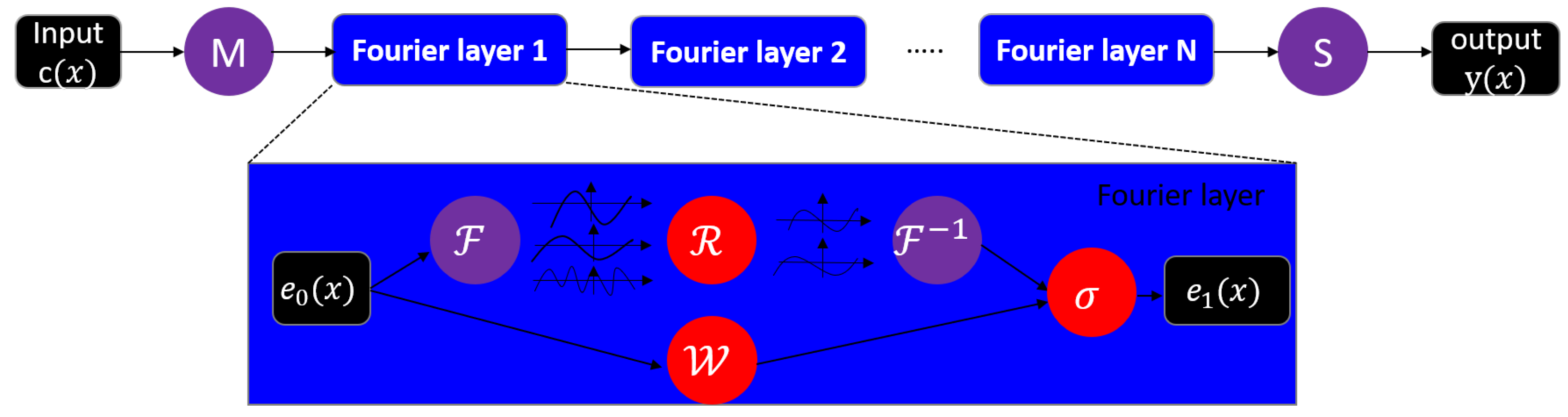
2.2. FNO Architecture

The Fourier neural operator is effective in learning the mapping relationships between the infinite-dimensional function spaces that convert a traditional convolutional operation into a multiplication operation using the Fourier transform [34]. This causes the higher modes of the neural layer to be removed from the Fourier space, leaving only the lower modes in the Fourier layer. Hence, FNO can greatly improve the computational efficiency of the training process. The goal of FNO is to use a neural network ${\mathcal{G}}^{†}\left(a\right)=u$ to approximate the mapping of function $\mathcal{G}:\mathcal{A}\to \mathcal{U}$, $\mathcal{G}\approx {\mathcal{G}}^{†}$.

Figure 1 shows the full FNO architecture; input observation $c\left(x\right)$ is first lifted to a higher dimensional potential representation $e_0\left(x\right)=M\left(c\left(x\right)\right)$ by fully-connected shallow neural network M. Then, $e_0\left(x\right)$ is used as input for an iterative Fourier layer $e_0\to e_1\to e_2\to \dots \to e_N$. The concrete iterative process from state $e_n\to e_{n+1}$ can be written as:

$$e_{n+1}\left(x\right)=\sigma (W{e}_n\left(x\right)+\left(\mathcal{K}(a;\varphi )e_n\left(x\right)\right)\left(x\right))$$

(5)

Here, $\sigma$ is a non-linear activation function, W is a linear transformation, and $\mathcal{K}$ is an integral kernel transformation parameterized by a neural network. ($\mathcal{K}(a;\varphi )e_n\left(x\right))\left(x\right)$ is the bias, that can be written as an integral:

$$\begin{array}{cc}\hfill \left(\mathcal{K}(a;\varphi )e_n\left(x\right)\right)\left(x\right)& \hfill =\int {\kappa }_{\varphi }(x,y)e_n\left(y\right)dy\hfill \end{array}$$

(6)

To accelerate the integration process $\int {\kappa }_{\varphi }(x,y)e_n\left(y\right)dy$ of Equation (6), Li et al. (2020) imposed a condition that is ${\kappa }_{\varphi }(x,y)={\kappa }_{\varphi }(x-y)$ and the new integral is [41]:

$$\begin{array}{cc}\hfill \left(\mathcal{K}(a;\varphi )e_n\left(x\right)\right)\left(x\right)& \hfill =\int {\kappa }_{\varphi }(x-y)e_n\left(y\right)dy\hfill \\ \hfill & \hfill ={\mathcal{F}}^{-1}\left(R_{\varphi }\left(\mathcal{F}{e}_n\right)\right)\left(x\right)\hfill \end{array}$$

(7)

where $\mathcal{F}$ denotes the Fourier transform, and ${\mathcal{F}}^{-1}$ denotes the inverse Fourier transform. $R_{\varphi }$ is a Fourier transform of periodic function $\kappa$, $R_{\varphi }=\mathcal{F}\left({\kappa }_{\varphi }\right)$, and ${\kappa }_{\varphi }$ is a the kernel of the neural network. Following the N Fourier layer iteration, the last state output $e_N\left(x\right)$ is projected back to the original space using a fully connected neural network S, $y\left(x\right)=S\left(e_N\left(x\right)\right)$.

In every block of the Fourier layer, FNO approximates highly non-linear functions mainly via combining the linear transform W and global integral operator $R_{\varphi }$ (Fourier transform). $R_{\varphi }$ can be parameterized as a complex-valued tensor in the Fourier space from truncating high Fourier frequency modes k, and it can greatly reduce the number of trainable parameters and improve efficiency during the process of training.

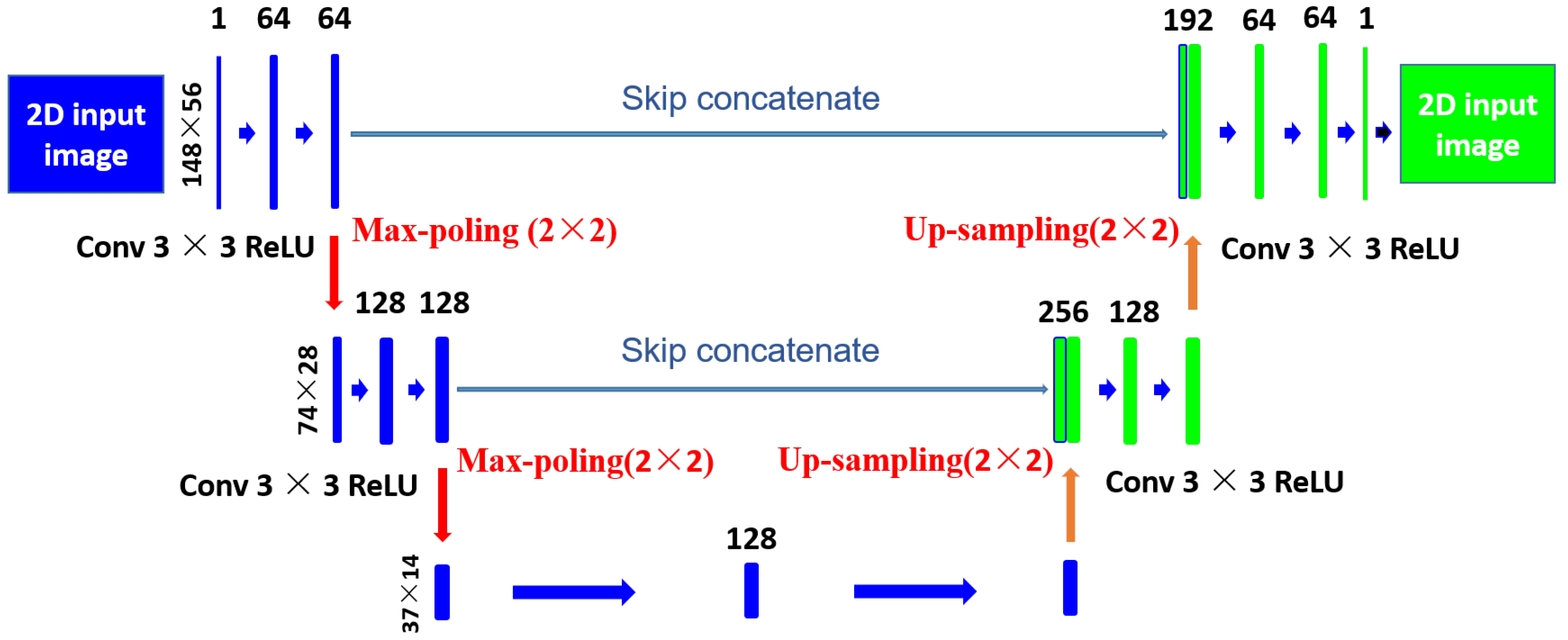
2.3. CNN Class Network Architecture

The convolutional neural network (CNN) evolved from a multi-layer perceptron (MLP) [42]. Due to its structural characteristics of a local region connection, weight sharing and downsampling, the convolutional neural network achieves excellent performance for image processing, and has been widely used in various fields. A typical CNN consists of three parts: The convolution layer, the pooling layer, and the fully connected layer. The convolution layer is responsible for extracting local features in the image. The pooling layer is used to greatly reduce the magnitude of the net parameters (dimension reduction); the fully connected layer is similar to the part of the traditional neural network, that is used to output results. The other CNN class network is a full convolutional neural network (FCN) [43]. The difference between the FCN and the CNN is that the latter’s full connection FC layer is replaced by the Conv. Therefore, images of any size can be input into FCN. U-net was proposed by Ronneberger in 2015 [44], and is a variant of the FCN. Comparing the FCN, one of the most outstanding contributions of U-net is its skip connection operation, that reduces the image details lost due to downsampling, thus helping the network to more accurately locate the image. In this study, We use U-net to complete the same test, and we also compare the performances of the FNO-net and U-net. The U-net still retained two main structures: encoder and decoder [45]. The detailed U-net architecture is shown in Figure 2. The blue arrow is a convolution block composed of a 3 × 3 convolution layer and a ReLU layer, that can be used to extract and output feature maps of the same size as the input image. The red arrow is 2 × 2 max pooling to extract the downsampled feature maps. The orange arrow is an up-convolution operation that can obtain an upsampled feature map. The grey arrow denotes the concatenation operation, and the main function is concatenating the feature maps (blue box) from the left with the right feature maps (green box).

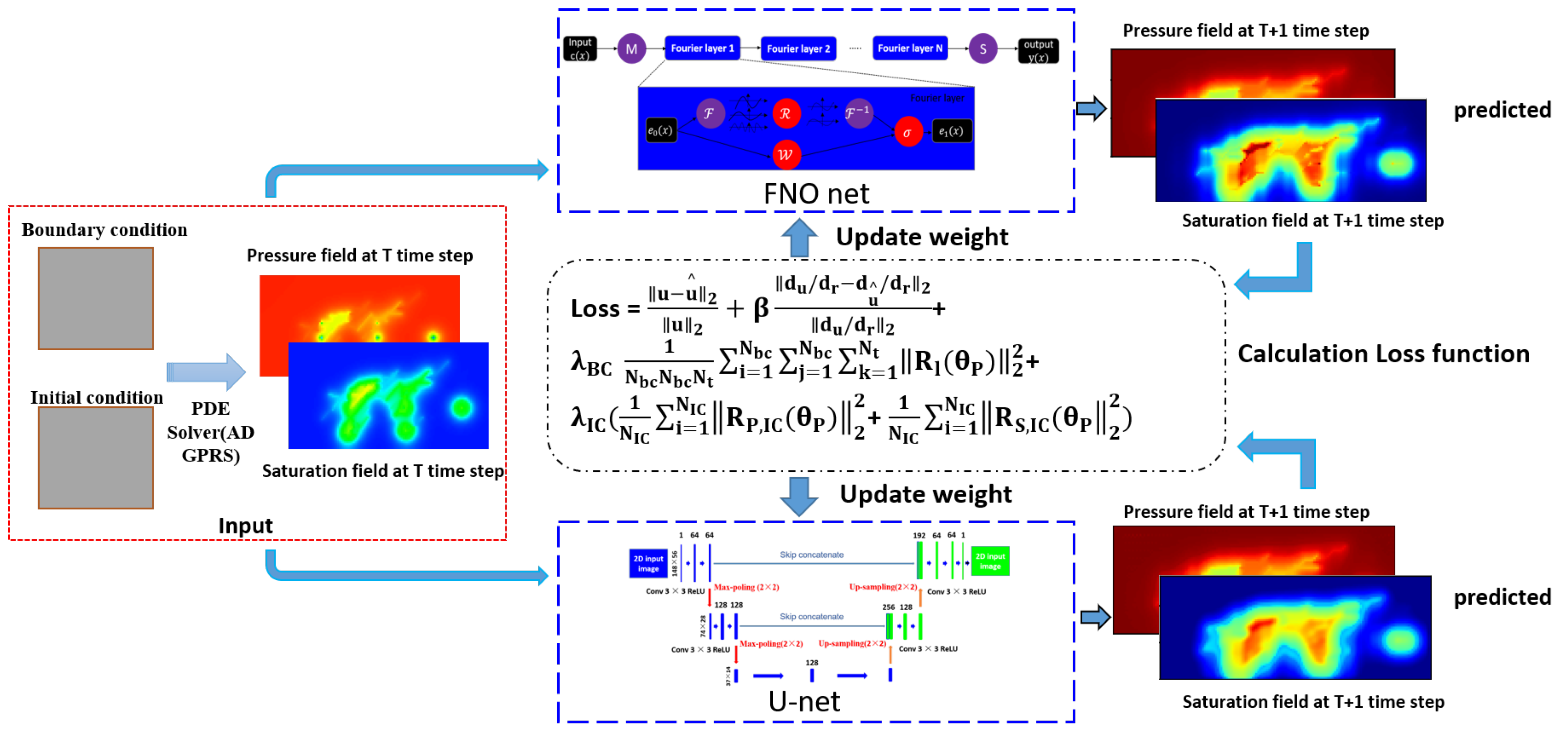
2.4. Training Details and Loss Function Design

In the current study, the Stanford in-house new generation reservoir simulator ADGPRS [46,47] was used to generate the simulation results of multi-phase flow in the heterogeneous reservoir with a complex fracture distribution. Permeability fields can be regarded as stochastic fields. The heterogeneity in the horizontal permeability $k_x$ is generated by Stanford Geo statistical Modeling Software (SGeMS) [48]. Permeability map $k_y$ is calculated by multiplying the $k_x$ map by the anisotropy map. The porosity map is perturbed with a random Gaussian noise $ϵ$ with a mean value of zero and a standard deviation of 0.005. In addition, four parameters are required to define the distribution of the natural fractures in numerical simulations: fracture coordinate position, depth, permeability, and porosity [40]. Then, the simulator runs, the field distribution of time step N can be divided into datasets to train the FNO model. There are two key hyper-parameters in FNO-net: firstly, the width of the convolution layer, that refers to the number of features learned at every Fourier layer; secondly, frequency mode k, that defines the number of lower Fourier modes retained after removing the high Fourier mode in the Fourier series expansion. The value of frequency mode k depends on the concrete size of the grid space. To predict the field distribution at time $t_{n+1}$ using only the simulation results at time $t_n$ as input data, the two hyper parameters of FNO need to be redefined. In this research, we assign the value of frequency mode $k=4$ and width as 1. The FNO-net structure of the training is illustrated in

Table 1. FNO-net structure for training. Padding denotes a padding operator that accommodates the non-periodic boundaries. Linear denotes the linear transformation to lift the input to the high dimensional space and the projection back to the original space. ${\mathcal{F}}_1$–${\mathcal{F}}_5$ denotes five Fourier layers.

Network Layer	Output Shape
Frequency mode k, width	(4, 1)
Input	$(1050,148,56,1,1)$
Padding	$(1050,148,56,32,1)$
Linear	$(1050,148,56,32,1)$
${\mathcal{F}}_1$:Fourier3d/conv3d/BatchNorm3d	$(1050,148,56,32,36)$
${\mathcal{F}}_2$:Fourier3d/conv3d/BatchNorm3d	$(1050,148,56,32,36)$
${\mathcal{F}}_3$:Fourier3d/conv3d/BatchNorm3d	$(1050,148,56,32,36)$
${\mathcal{F}}_4$:Fourier3d/conv3d/BatchNorm3d	$(1050,148,56,32,36)$
${\mathcal{F}}_5$:Fourier3d/conv3d/BatchNorm3d	$(1050,148,56,32,36)$
Projection1	$(1050,148,56,32,128)$
Projection2	$(1050,148,56,32,1)$
Output	$(1050,148,56,1,1)$

. The details of the data preparation are described in Section 3.

The total loss function for the FNO-net in this study can be divided into three parts: $L_2$-loss. The $L_2$ norm can prevent over-fitting and improves the generalization ability of the model; BC (boundary condition)-loss; IC (initial condition)-loss. The total loss function is written as:

$$Los{s}_{total}=L_2(u,\widehat{u})+{\lambda }_{1}Los{s}_{BC}+{\lambda }_{2}Los{s}_{IC}$$

(8)

The $L_2$-loss:

$$L_2(u,\widehat{u})=\frac{\parallel u-\widehat{u}{\parallel }_2}{{\parallel u\parallel }_2}+\beta \frac{\parallel d_u/d_r-d_{\widehat{u}}/d_r{\parallel }_2}{\parallel d_u/d_r{\parallel }_2}$$

(9)

$L_2$ norm is mainly minimizing the mean squared error between prediction $\widehat{u}$ and ground truth u. Where $d_u/d_r$ is the first derivative of the data, $d_{\widehat{u}}/d_r$ is the first derivative of the predicted output, ${\parallel \parallel }_2$ is the $L_2$ norm, and $\beta$ is a hyper-parameter. The relative $L_2$-loss can prevent over-fitting and improve the generalization ability of the model, especially when the training data have large variances in the norm [49].

For our test case, the boundary conditions are four Newman boundaries. Newman boundary conditions can be written as:

$$K\left(\mathbf{x}\right)\nabla h\left(\mathbf{x}\right)\mathbf{n}\left(\mathbf{x}\right)=0,\mathbf{x}\in {\mathrm{\Gamma }}_N$$

(10)

Equation (10) denotes the Newman boundary condition. The pressure cannot be transmitted outward through the boundary, that is, its derivative in the direction of the outward normal is limited to zero. K(x) denotes the hydraulic conductivity; h(x) denotes the hydraulic head; n(x) denotes an outward unit vector that is normal to the boundary with the model parameters, such as hydraulic conductivity K(x), which is available, and the boundary and initial conditions are specified; therefore, the problems can be solved with numerical simulators.

$$Los{s}_{BC}\left({\theta }_P\right)=\frac{1}{N_{bc}{N}_{bc}{N}_t}\sum _{i=1}^{N_{bc}}\sum _{j=1}^{N_{bc}}\sum _{k=1}^{N_t}{∥R_l\left({\theta }_P\right)∥}_2^2$$

(11)

Equation (11) denotes the loss function of the boundary condition. $N_{bc}$ is the number of the test point in the boundaries. $N_t$ is the number of the time step in the test case. $R_l\left({\theta }_P\right)$ represents the residual of Equation (10) for phase l.

$$R_{P,IC}\left({\theta }_P\right)=\widehat{P}\left({\theta }_P\right)-P\left({\theta }_P\right)$$

(12)

$$R_{S,IC}\left({\theta }_S\right)=\widehat{S}\left({\theta }_S\right)-S\left({\theta }_S\right)$$

(13)

Equations (15) and (16) are the difference between the predicted value and the initial value, respectively. $R_{P,IC}$ is the pressure residual. $R_{S,IC}$ is the saturation residual.

$$Los{s}_{IC}=\frac{1}{N_{IC}}\sum _{i=1}^{N_{IC}}{∥R_{P,IC}\left({\theta }_P\right)∥}_2^2+\frac{1}{N_{IC}}\sum _{i=1}^{N_{IC}}{∥R_{S,IC}\left({\theta }_S\right)∥}_2^2$$

(14)

Equation (14) denotes the loss function of the initial condition. The parameters of the network are optimized by minimizing the above total loss function with the adaptive moment estimation (Adam) optimization algorithm [50]. The initial hyper-parameter $\beta$ is 1. In the training process, the initial learning rate is 0.001 and the learning rate gradually decreases with a certain step and reduction rate. Training stops when the total loss no longer decreases.

For U-net, the same datasets were used as input data for training and prediction. The U-net structure designed for this study is shown in

Table 2. The network architectures of U-net. The convolutional layer kernel size, stride, and padding are (3, 3), (1, 1), and 1. ReLU is a rectified linear layer; MaxPool2d represents a downsample layer with kernel size (2, 2) and strides (2, 2); upsampled denotes an upsample layer with scale factor 2.

Network Layer	Output Shape
Input	$(1,148,56)$
Conv2d/ReLu/Conv2d/ReLu	$(64,148,56)$
MaxPool2d/ Conv2d/ReLu/Conv2d/ReLu	$(128,74,28)$
MaxPool2d/ Conv2d/ReLu/Conv2d/ReLu	$(128,37,14)$
Conv2d/ReLu/Conv2d/ReLu	$(128,37,14)$
Conv2d/ReLu/Conv2d/ReLu	$(128,37,14)$
Upsampled/Conv2d/ReLu/Conv2d/ReLu	$(256,74,28)$
Upsampled/Conv2d/ReLu/Conv2d/ReLu	$(192,148,56)$
Conv2d/ReLu/Conv2d/ReLu	$(64,148,56)$
Output	$(1,148,56)$

. Considering the large difference between the pressure and saturation values, we normalized the pressure field data in the training. The learning rate of the model is modified dynamically with a decrement multiple of 0.1 and an interval of 20 epochs. The most common loss function mean squared error (MSE) was selected. The MSE loss is the square of the difference between predictions and the ground truth, and it averages it out across the whole dataset. MSE can be written as:

$$\mathrm{MSE}=\frac{1}{N}\sum _{i=1}^N{\left(u_i-{\widehat{u}}_i\right)}^2$$

(15)

$$Los{s}_{U-net}=\mathrm{MSE}+{\lambda }_{3}Los{s}_{BC}+{\lambda }_{4}Los{s}_{IC}$$

(16)

where N is the number of samples we are testing against, $u_i$ are the true values, and ${\widehat{u}}_i$ are the prediction values. To test the effect of the boundary condition and initial condition constraint on the model accuracy, we also added BC and IC parts in the $U-net$ loss function.

Figure 3 presents a flowchart that shows the deep learning (DL) procedure in multiphase flow. Firstly, the distribution of pressure and saturation fields at time step T is used as input data for FNO and U-NET. Secondly, the network outputs the predicted values of pressure and the saturation fields at time step T + 1 through training. Then, the loss function, considering the constraints of the initial conditions and boundary conditions, is calculated by Equations (8) and (16). The network weight is updated through backward propagation.

Now, we introduce several error metrics, that will be used to evaluate the performance of the model. The relative error for the predicted results is defined as:

$$A_i=\frac{1}{T}\frac{1}{N}\sum _{t=1}^T\sum _{n=1}^N\left|u_i-{\widehat{u}}_i\right|$$

(17)

$$a_i=\frac{1}{T}\frac{1}{N}\sum _{t=1}^T\sum _{n=1}^N\left|u_i\right|$$

(18)

$$R{E}_i=\frac{A_i}{a_i}$$

(19)

where T represents the number of the simulated time steps, N represents the number of grids, $u_i$ represents the actual value, such as the gas saturation distribution and pressure, and ${\widehat{u}}_i$ represents the corresponding predicted value in the output. Variable $A_i$ is the average absolute error, $a_i$ is the average of the actual value, and $R{E}_i$ represents the relative error.

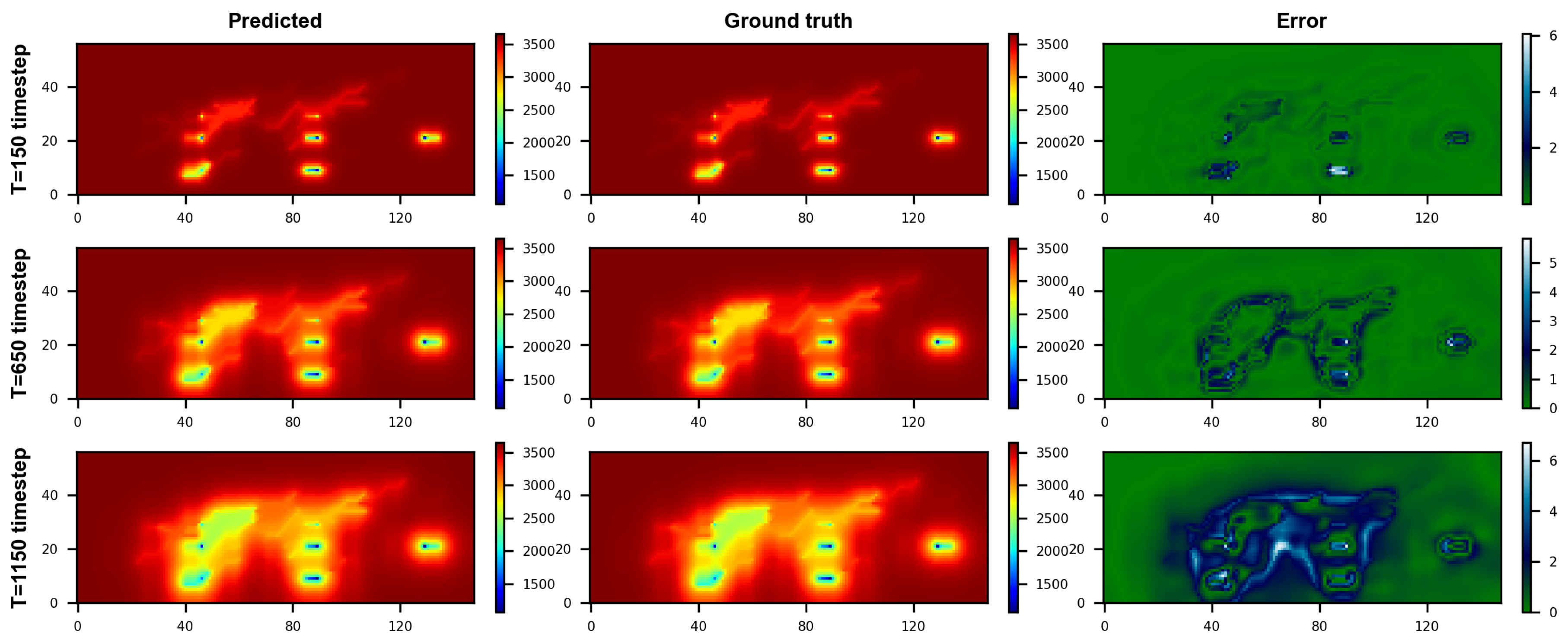
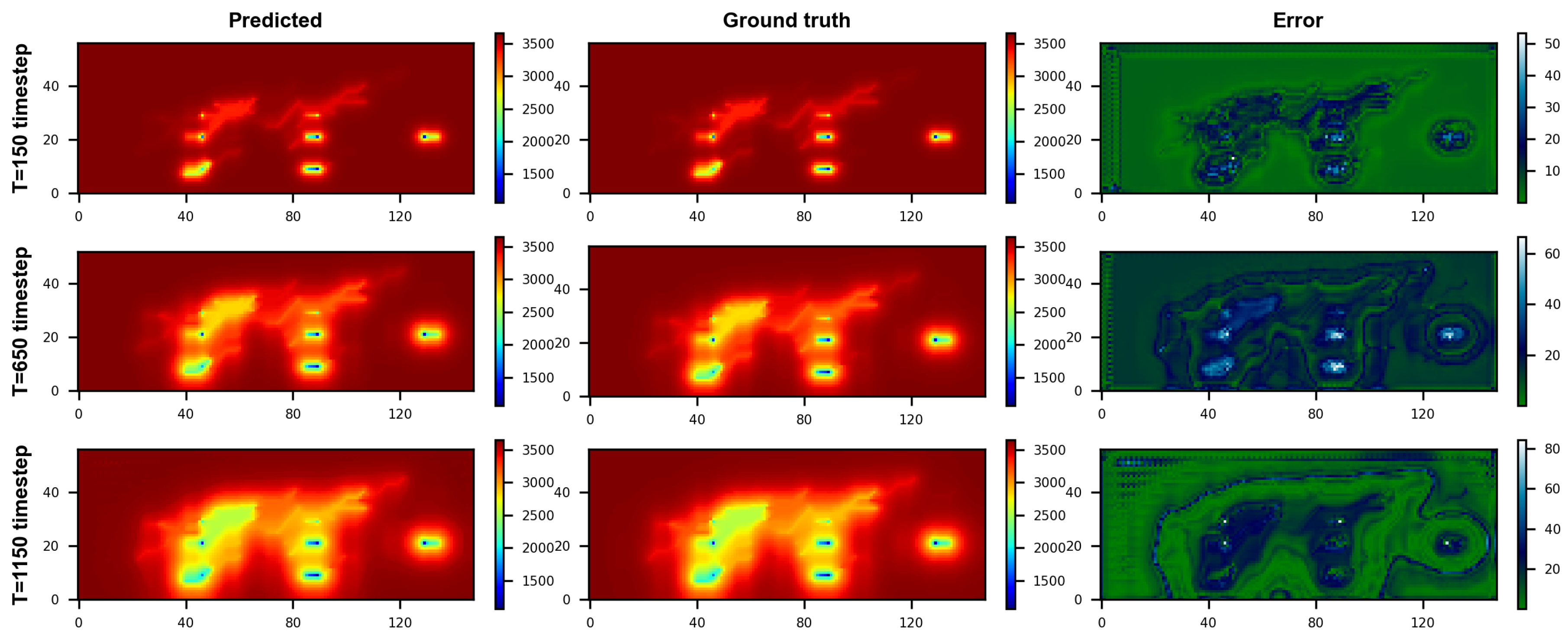
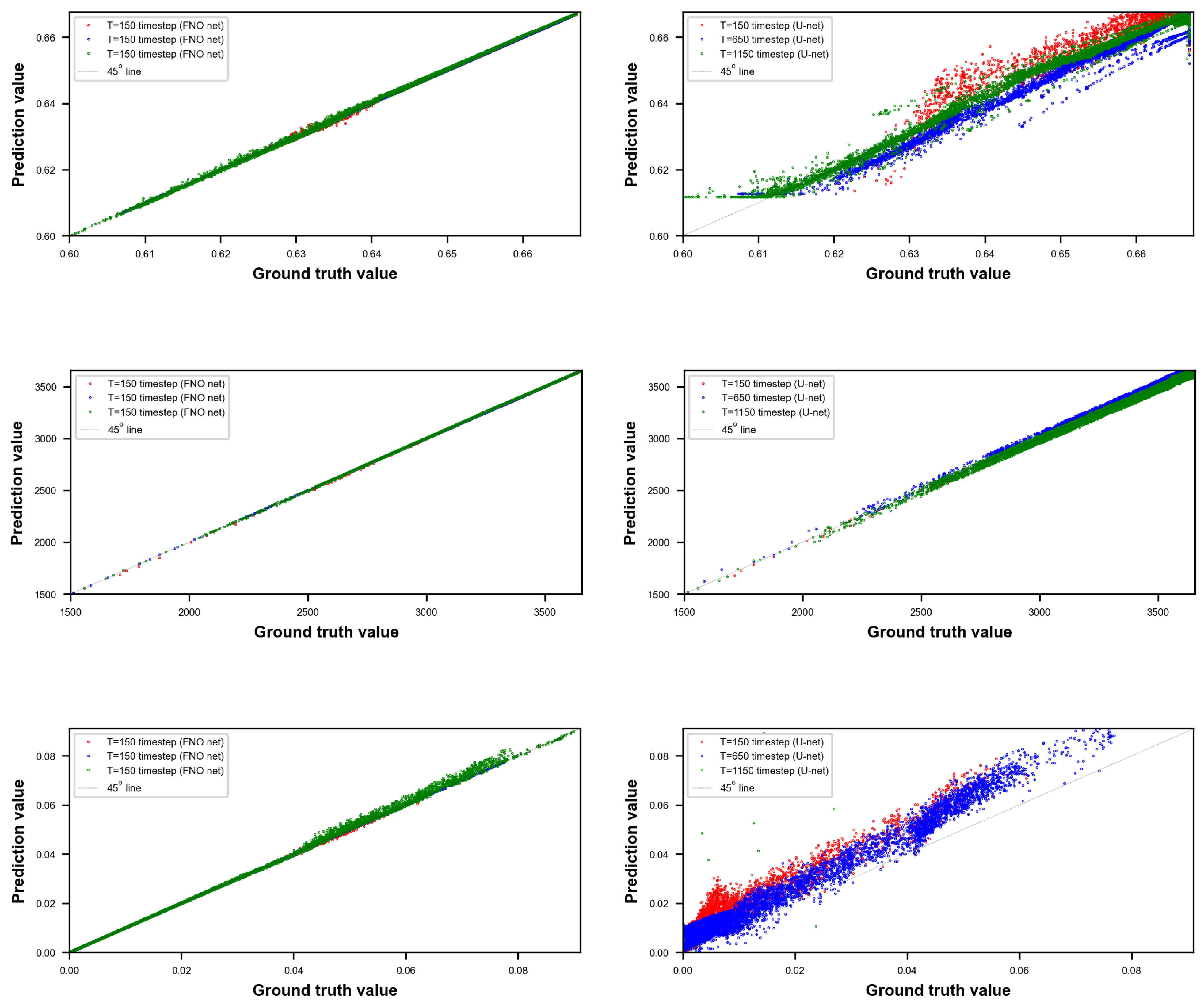
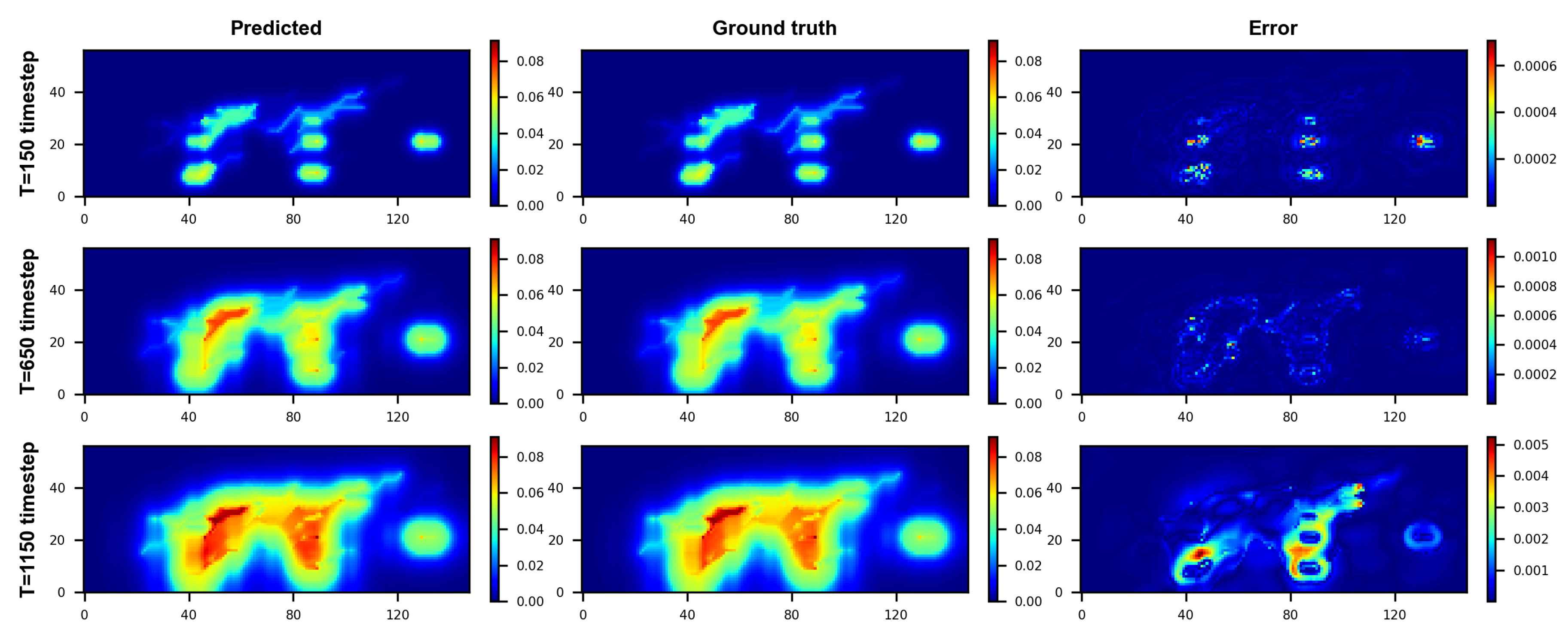
3. Results and Discussion

In this section, we demonstrate the simulation performance of FNO-net and U-net in 2D multi-phase subsurface flow in a fractured reservoir. The test case was a 2D (1480 ft × 560 ft) heterogeneous reservoir with a complex fracture. The numerical simulation results were obtained from the Stanford new generation reservoir simulator ADGPRS. Once the simulation completed its run, the simulation results, such as pressure and saturation field distributions were divided into datasets. Then, the FNO network performed training and prediction. In addition, we evaluated the performance of the FNO and U-net models in predicting the same test case from the aspects of runtimes and accuracy. The details of data processing (pre- and post-processing) and model training are described for the case, as follows. We made predictions and error metrics for saturation and pressure.

The implementation of the FNO neural network and U-net in this paper is based on the popular open-source software library, PyTorch, for machine learning. The test case in this study was performed on the DELL Precision T7920 workstation with 2 Inter(R) Xeon(R) Gold 6230R CPU@ 2.10 GHz, and 2 NVIDIA 3090 GPU. All codes and data required to reproduce the results and presented in the paper will be available at https://github.com/HPMPS (accessed on 21 April 2023) upon publication.

The test reservoir domain was discretized using the Cartesian grid, with 148 × 56 grid cells in the x and y directions. The total number of grids was 7395 with seven production wells. All production well coordinates were (47, 22), (90, 22), (130, 20), (90, 30), (90, 10), (47, 10), and (47, 30). The oil production rate was 14.7 STB/day in every production well control. We used SGeMS’s sequential Gaussian simulation to generate permeability fields ($k_x$, $k_y$) with a 148 × 56 grid size.

Figure 4 shows $k_x$ and $k_y$. The well configuration in the 2D reservoir is shown in Figure 5a. Forty-two natural fractures were also added to the heterogeneous reservoir. The 42 natural fractures have been defined by the coordinates method in this reservoir modeling. The concrete parameters of these fractures, including position, permeability in horizontal directions, permeability in vertical directions, porosity in fracture, and aperture of fracture are listed in

Table A1. Parameters of the natural fractures in the simulated case study.

Natural Fracture	PERM (mD)	PERMV (mD)	PORO	APERTURE
$Fracture1$	120	1.5	0.9	0.02
$Fracture2$	400	12.5	0.5	0.04
$Fracture3$	180	10.5	0.4	0.1
$Fracture4$	240	4.5	0.19	0.02
$Fracture5$	185	6.5	0.16	0.08
$Fracture6$	255	7.3	0.55	0.2
$Fracture7$	860	1.5	0.19	0.25
$Fracture8$	385	4.5	0.29	0.25
$Fracture9$	722	3.5	0.29	0.52
$Fracture10$	486	4.7	0.39	0.48
$Fracture11$	510	2.6	0.69	0.83
$Fracture12$	130	1.2	0.74	0.55
$Fracture13$	558	1.3	0.98	0.35
$Fracture14$	650	1.55	0.78	0.53
$Fracture15$	255	1.57	0.75	0.08
$Fracture16$	257	1.35	0.5	0.07
$Fracture17$	357	1.55	0.94	0.07
$Fracture18$	457	1.45	0.93	0.06
$Fracture19$	557	1.75	0.98	0.05
$Fracture20$	740	1.65	0.89	0.04
$Fracture21$	670	10.5	0.85	0.03
$Fracture22$	470	12.5	0.5	0.03
$Fracture23$	650	11.6	0.3	0.03
$Fracture24$	453	8.56	0.4	0.02
$Fracture25$	350	7.56	0.5	0.01
$Fracture26$	620	6.53	0.54	0.1
$Fracture27$	320	8.53	0.44	0.11
$Fracture28$	280	5.55	0.4	0.25
$Fracture29$	356	2.65	0.3	0.11
$Fracture30$	455	7.52	0.2	0.32
$Fracture31$	456	1.45	0.93	0.06
$Fracture32$	655	1.75	0.98	0.05
$Fracture33$	725	1.65	0.89	0.04
$Fracture34$	680	10.5	0.85	0.03
$Fracture35$	450	12.5	0.5	0.03
$Fracture36$	680	11.6	0.3	0.03
$Fracture37$	475	8.56	0.4	0.02
$Fracture38$	356	7.56	0.5	0.01
$Fracture39$	653	6.53	0.54	0.1
$Fracture40$	258	8.53	0.44	0.11
$Fracture41$	655	5.55	0.4	0.25
$Fracture42$	455	2.65	0.3	0.11

. The distribution of these fractures is plotted in Figure 5a. In Figure 5b, krow is the relative permeability of oil in a two-phase oil-water system, krw is the relative permeability of water in a two-phase oil-water system, krog is the relative permeability of oil in a two-phase gas-oil system, and krg is the relative permeability of gas in a two-phase gas-oil system.

Once the numerical model was built, the ADGPRS simulator ran for 5255 days with 1051 time steps, and 5 days for each time step. Then, the simulation results were generated, including the pressure, oil saturation, and water saturation distribution, and these results were used as input data for the FNO network for training. In the training process, the FNO network training, testing, and validation are described as follows. The dataset organization involved each batch with consecutive two time steps, batch 1 was one to two time steps, batch 2 was two to three time steps, and so on. The last one was 1049 to 1050 time steps, the total batch number was 1050. Figure 6 illustrates the preparation of the batches. For the first batch, the values of the one time step were used as input data to train the FNO-net and the predicted $\widehat{u}$ values in Equation (9). Then, the values in the two time steps were also introduced in Equation (9) as truth values u to calculate the $L_2$ loss function in the equation. By combining the $BC$ loss and $IC$ loss, we optimized the total loss in Equation (8) using the Adam optimization method. Among the 1000 batches, 800 batches were randomly selected as the training set and the remaining 200 batches as the testing set. To demonstrate the prediction capability in the time series, the values in the three 150, 650, and 1150 time steps were used as the validation data and were excluded from training and testing. The procedure of data preparation for U-net was the same as that for FNO-net.

The input shape for the FNO network was $(1050,148,56,1,1)$, where 1050 was the number of samples, 145 was the number of grids in the x-dimension, 51 was the number of grids in the y-dimension, one was the required place holder for the variables, and one was the first one time step in the time series. The output shape was $(1050,148,56,1)$, where one was the sequential one time step. The input shape for U-net was (1050, 148, 56) and the output shape was (1050, 148, 56). The same test case of multiphase flow in a fractured reservoir is the benchmark to compare the computational cost of FNO and U-net. The results are shown in

Table 3. Comparison of the performance between FNO and U-net models.

Model	Per Epoch Time (s)	Ease of Use	Order of Error	The Ability to Describe Fractures
FNO-net	2.6	Easy	${10}^{-3}$	Fully describe
U-net	51.2	Easy	${10}^{-2}$	Partially describe

. For FNO networks, it takes about 1300 s to train 500 epochs using 1051 time step data in an NVIDIA GeForce GTX 3090 Ti GPU computer. Each epoch takes 2.6 s. To the contrary, U-net takes about 25,612 s to train 500 epochs, with each epoch taking 51.2 s. The comparative results of FNO and U-net in terms of accuracy, ease of use, and ability to describe fractures are presented in Table 3.

The performance of the constructed FNO-net and U-net models are evaluated here. Figure 7 and Figure 8 represent the prediction results of oil saturation at T = 150 time steps, 650 time steps, and 1150 time steps by FNO and U-net, respectively. As Figure 7 shows, the average difference between the ground truth value and the predicted value is ${10}^{-3}$ by FNO. Figure 8 shows that the average difference between the ground truth value and the predicted value is ${10}^{-2}$ by U-net. The error of U-net is 10 times larger than FNO-net. FNO achieved the best performance. In comparison with the first row from Figure 7 and Figure 8, FNO can accurately depict the influence of fine fractures, while U-net can hardly depict this phenomenon. These results show that FNO has a better ability to capture the influence of fractures. The third column error graph in Figure 7 and Figure 8 displays that the errors of the FNO model mainly exist near the production well. To improve the prediction in this narrow area, one approach is that the training data are denser in this area. In addition, it can be found that U-net has very poor performance at the boundary in Figure 8, while FNO can better predict the saturation distribution at the boundary. These error results show that adding the boundary condition and the initial condition constraints to the loss function have a positive effect on the predicted oil saturation.

Figure 9 displays the predicted pressure distribution by FNO-net for the test case at the time steps of 50 (first row), 250 (second row), and 450 (third row), respectively. Figure 9 shows that the FNO model achieves approximation accuracy for the strongly non-linear and discontinuous pressure field, as expected. The maximum difference between the ground truth value and the predicted value is 6 psi by FNO, although the pressure field truth value varies from 1000 psi to 3000 psi. Comparing the predicted results by U-net in Figure 10, the maximum difference between the ground truth value and the predicted value reaches 80 psi. The error of U-net is 13 times larger than FNO-net. FNO also achieved better performance in the prediction of pressure distribution. The error results in Figure 10 also show that U-net has very poor performance at the boundary.

In this test case, the variation ranges for the oil phase saturation, gas phase saturation, and pressure truth value are, respectively, (0, 1), (0, 0.091), and (1000 psi, 3000 psi). This mixed complex scale greatly increases the difficulty of the deep learning model prediction. To test the predicted ability of two networks in the fractured reservoir in detail, we present cross plots of the predicted and ground truth values for three test time steps in Figure 11. The left column of Figure 11 presents the FNO results and the right column shows the U-net results. The left column in Figure 11 shows that all test points of FNO for oil saturation, gas saturation, and pressure fall near line 45${}^{\circ }$, which demonstrates that FNO-net solutions are in close agreement with the ground truth values. Among them, the prediction error of FNO for gas saturation is the largest, these results show that the capacity of the FNO model to treat fractured reservoirs is sufficient to meet engineering requirements. The right column of Figure 11 illustrates U-net’s poor performance in predicting oil saturation, and especially gas saturation. The first figure in the right column of Figure 11 shows that the predicted value of oil saturation deviates abnormally near 0.6, which may be caused by not adding the constraints of the initial conditions and boundary conditions into the loss function of the U-net model. If we add the constraints of the initial conditions and boundary conditions to the U-net loss function, the model can better describe the local non-linear characteristics of the boundary and the accuracy of the gas saturation in the front.

For gas saturation distribution, the ground truth value varies from 0 to 0.0091. We also tested the reconstruction ability of the two networks on such a small scale. Figure 12 illustrates the predicted results of gas saturation using FNO-net, it can found that the maximum error is 0.006. Figure 13 shows that the U-net model reconstruction performance of the gas saturation is poor, especially near the fractures, with an overall maximum error of 0.02, which is more than 20 percent. This accuracy is not enough for the method to be applied to simulate the subsurface flow in fractured systems.

4. Conclusions

Classic CNN-based deep learning methods, such as U-net attempt to learn mappings between finite-dimensional Euclidean spaces, making them confined to a particular discretization. Moreover, the FNO tries to learn function-to-function mappings directly, which enables FNO to have a better generalization ability to deal with time series problems and predict future time step states through historical time step states. In this study, two deep learning models FNO and U-net were constructed to predict in 2D, the three-phase subsurface flow in a complex fracture reservoir. Compared with the results of pressure, oil saturation, and gas saturation field distributions, The FNO-net provided better prediction performance than the U-net in predicting the flow process precisely and quickly. The results show that FNO has a better ability than U-net to describe the influence of fractures, and U-net can hardly depict this phenomenon. In addition, it is essential to add the physical constraints of the initial conditions and boundary conditions to the loss function of the pure data-driven model to improve the predictive performance of the model.

Key achievements in this work:

• Our work successfully implemented two current advanced deep learning models to predict subsurface flow in complex fractured reservoirs. The performance of the two models was evaluated from the aspects of computational cost, accuracy, and fracture description;
• By adding initial conditions and boundary conditions to the network loss function, we proved the necessity of adding physical constraints to the data-driven model;
• This work contributes to advancing the understanding of the applicability of FNO-net, and provides new insights into deep learning methods for predicting multiphase flow in complex fractured reservoirs.

References

1. Mardashov, D.; Duryagin, V.; Islamov, S. Technology for improving the efficiency of fractured reservoir development using gel-forming compositions. Energies 2021, 14, 8254. [Google Scholar] [CrossRef]
2. Cao, M.; Sharma, M. An Efficient Model of Simulating Fracture Propagation and Energy Recovery from Naturally Fractured Reservoirs: Effect of Fracture Geometry, Topology and Connectivity. In Proceedings of the SPE Hydraulic Fracturing Technology Conference and Exhibition, The Woodlands, TX, USA, 31 January–2 February 2023. [Google Scholar]
3. Ding, M.; Gao, M.; Wang, Y.; Qu, Z.; Chen, X. Experimental study on CO2-EOR in fractured reservoirs: Influence of fracture density, miscibility and production scheme. J. Pet. Sci. Eng. 2019, 174, 476–485. [Google Scholar] [CrossRef]
4. van Golf-Racht, T.D. Fundamentals of Fractured Reservoir Engineering; Elsevier: Amsterdam, The Netherlands, 1982. [Google Scholar]
5. Gilman, J.R.; Kazemi, H. Improvements in simulation of naturally fractured reservoirs. Soc. Pet. Eng. J. 1983, 23, 695–707. [Google Scholar] [CrossRef]
6. Hawez, H.; Sanaee, R.; Faisal, N. Multiphase Flow Modelling in Fractured Reservoirs Using a Novel Computational Fluid Dynamics Approach. In Proceedings of the 55th US Rock Mechanics/Geomechanics Symposium, Online, 18–25 June 2021; OnePetro: Richardson, TX, USA, 2021. [Google Scholar]
7. Wu, Y.S. On the effective continuum method for modeling multiphase flow, multicomponent transport, and heat transfer in fractured rock. Dynamics of Fluids in Fractured Rock; John Wiley & Sons, Inc.: New York, NY, USA, 2013. [Google Scholar]
8. Warren, J.; Root, P.J. The behavior of naturally fractured reservoirs. Soc. Pet. Eng. J. 1963, 3, 245–255. [Google Scholar] [CrossRef]
9. Kazemi, H. Pressure transient analysis of naturally fractured reservoirs with uniform fracture distribution. Soc. Pet. Eng. J. 1969, 9, 451–462. [Google Scholar] [CrossRef]
10. Civan, F.; Rai, C.S.; Sondergeld, C.H. Shale-gas permeability and diffusivity inferred by improved formulation of relevant retention and transport mechanisms. Transp. Porous Media 2011, 86, 925–944. [Google Scholar] [CrossRef]
11. Dehghanpour, H.; Shirdel, M. A triple porosity model for shale gas reservoirs. In Proceedings of the Canadian Unconventional Resources Conference, Houston, TX, USA, 26–28 July 2021; OnePetro: Richardson, TX, USA, 2011. [Google Scholar]
12. Yan, B.; Wang, Y.; Killough, J.E. Beyond dual-porosity modeling for the simulation of complex flow mechanisms in shale reservoirs. Comput. Geosci. 2016, 20, 69–91. [Google Scholar] [CrossRef]
13. Xu, Z.; Huang, Z.; Yang, Y. The hybrid-dimensional Darcy’s law: A non-conforming reinterpreted discrete fracture model (RDFM) for single-phase flow in fractured media. J. Comput. Phys. 2023, 473, 111749. [Google Scholar] [CrossRef]
14. Koohbor, B.; Fahs, M.; Hoteit, H.; Doummar, J.; Younes, A.; Belfort, B. An advanced discrete fracture model for variably saturated flow in fractured porous media. Adv. Water Resour. 2020, 140, 103602. [Google Scholar] [CrossRef]
15. Garipov, T.; Karimi-Fard, M.; Tchelepi, H. Discrete fracture model for coupled flow and geomechanics. Comput. Geosci. 2016, 20, 149–160. [Google Scholar] [CrossRef]
16. Wang, L.; Golfier, F.; Tinet, A.J.; Chen, W.; Vuik, C. An efficient adaptive implicit scheme with equivalent continuum approach for two-phase flow in fractured vuggy porous media. Adv. Water Resour. 2022, 163, 104186. [Google Scholar] [CrossRef]
17. Xiong, X.; Devegowda, D.; Michel, G.; Sigal, R.F.; Civan, F. A fully-coupled free and adsorptive phase transport model for shale gas reservoirs including non-Darcy flow effects. In Proceedings of the SPE Annual Technical Conference and Exhibition, San Antonio, TX, USA, 8–10 October 2012; OnePetro: Richardson, TX, USA, 2012. [Google Scholar]
18. Snow, D.T. A Parallel Plate Model of Fractured Permeable Media; University of California: Berkeley, CA, USA, 1965. [Google Scholar]
19. Moinfar, A.; Varavei, A.; Sepehrnoori, K.; Johns, R.T. Development of an efficient embedded discrete fracture model for 3D compositional reservoir simulation in fractured reservoirs. SPE J. 2014, 19, 289–303. [Google Scholar] [CrossRef]
20. Ţene, M.; Bosma, S.B.; Al Kobaisi, M.S.; Hajibeygi, H. Projection-based embedded discrete fracture model (pEDFM). Adv. Water Resour. 2017, 105, 205–216. [Google Scholar] [CrossRef]
21. Fang, S.; Cheng, L.; Ayala, L.F. A coupled boundary element and finite element method for the analysis of flow through fractured porous media. J. Pet. Sci. Eng. 2017, 152, 375–390. [Google Scholar] [CrossRef]
22. Du, X.; Cheng, L.; Liu, Y.; Rao, X.; Ma, M.; Cao, R.; Zhou, J. Application of 3D embedded discrete fracture model for simulating CO2-EOR and geological storage in fractured reservoirs. IOP Conf. Ser. Earth Environ. Sci. 2020, 467, 012013. [Google Scholar] [CrossRef]
23. Matthäi, S.K.; Mezentsev, A.; Belayneh, M. Control-volume finite-element two-phase flow experiments with fractured rock represented by unstructured 3D hybrid meshes. In Proceedings of the SPE Reservoir Simulation Symposium, Houston, TX, USA, 31 January–2 February 2005; OnePetro: Richardson, TX, USA, 2005. [Google Scholar]
24. D’Angelo, C.; Scotti, A. A mixed finite element method for Darcy flow in fractured porous media with non-matching grids. ESAIM Math. Model. Numer. Anal. 2012, 46, 465–489. [Google Scholar] [CrossRef]
25. Chu, A.K.; Benson, S.M.; Wen, G. Deep-Learning-Based Flow Prediction for CO2 Storage in Shale–Sandstone Formations. Energies 2023, 16, 246. [Google Scholar] [CrossRef]
26. He, X.; Santoso, R.; Hoteit, H. Application of machine-learning to construct equivalent continuum models from high-resolution discrete-fracture models. In Proceedings of the International Petroleum Technology Conference, Dhahran, Saudi Arabia, 13–15 January 2020; OnePetro: Richardson, TX, USA, 2020. [Google Scholar]
27. Xu, H.; Zhang, D.; Zeng, J. Deep-learning of parametric partial differential equations from sparse and noisy data. Phys. Fluids 2021, 33, 037132. [Google Scholar] [CrossRef]
28. Raissi, M.; Perdikaris, P.; Karniadakis, G.E. Physics-informed neural networks: A deep learning framework for solving forward and inverse problems involving nonlinear partial differential equations. J. Comput. Phys. 2019, 378, 686–707. [Google Scholar] [CrossRef]
29. Pan, S.; Duraisamy, K. Physics-informed probabilistic learning of linear embeddings of nonlinear dynamics with guaranteed stability. SIAM J. Appl. Dyn. Syst. 2020, 19, 480–509. [Google Scholar] [CrossRef]
30. Mo, S.; Zhu, Y.; Zabaras, N.; Shi, X.; Wu, J. Deep convolutional encoder-decoder networks for uncertainty quantification of dynamic multiphase flow in heterogeneous media. Water Resour. Res. 2019, 55, 703–728. [Google Scholar] [CrossRef]
31. Tan, X.; Chen, W.; Qin, C.; Zhao, W.; Ye, W. Characterisation for spatial distribution of mining-induced stress through deep learning algorithm on SHM data. Georisk: Assess. Manag. Risk Eng. Syst. Geohazards 2023, 17, 217–226. [Google Scholar] [CrossRef]
32. Takbiri-Borujeni, A.; Kazemi, H.; Nasrabadi, N. A data-driven surrogate to image-based flow simulations in porous media. Comput. Fluids 2020, 201, 104475. [Google Scholar] [CrossRef]
33. Wang, N.; Chang, H.; Zhang, D. Surrogate and inverse modeling for two-phase flow in porous media via theory-guided convolutional neural network. J. Comput. Phys. 2022, 466, 111419. [Google Scholar] [CrossRef]
34. Li, Z.; Kovachki, N.; Azizzadenesheli, K.; Liu, B.; Bhattacharya, K.; Stuart, A.; Anandkumar, A. Fourier neural operator for parametric partial differential equations. arXiv 2020, arXiv:2010.08895. [Google Scholar]
35. Wen, G.; Li, Z.; Azizzadenesheli, K.; Anandkumar, A.; Benson, S.M. U-FNO—An enhanced Fourier neural operator-based deep-learning model for multiphase flow. Adv. Water Resour. 2022, 163, 104180. [Google Scholar] [CrossRef]
36. Zhang, K.; Zuo, Y.; Zhao, H.; Ma, X.; Gu, J.; Wang, J.; Yang, Y.; Yao, C.; Yao, J. Fourier neural operator for solving subsurface oil/water two-phase flow partial differential equation. SPE J. 2022, 27, 1815–1830. [Google Scholar] [CrossRef]
37. Coats, K.H.; Thomas, L.; Pierson, R. Compositional and black oil reservoir simulation. In Proceedings of the SPE Reservoir Simulation Symposium, San Antonio, TX, USA, 12–15 February 1995; OnePetro: Richardson, TX, USA, 1995. [Google Scholar]
38. Chen, Z. Formulations and numerical methods of the black oil model in porous media. SIAM J. Numer. Anal. 2000, 38, 489–514. [Google Scholar] [CrossRef]
39. Li, J.; Tomin, P.; Tchelepi, H. Sequential fully implicit newton method for flow and transport with natural black-oil formulation. Comput. Geosci. 2023. [Google Scholar] [CrossRef]
40. Li, L.; Lee, S.H. Efficient field-scale simulation of black oil in a naturally fractured reservoir through discrete fracture networks and homogenized media. SPE Reserv. Eval. Eng. 2008, 11, 750–758. [Google Scholar] [CrossRef]
41. Li, Z.; Kovachki, N.; Azizzadenesheli, K.; Liu, B.; Bhattacharya, K.; Stuart, A.; Anandkumar, A. Neural operator: Graph kernel network for partial differential equations. arXiv 2020, arXiv:2003.03485. [Google Scholar]
42. LeCun, Y.; Bottou, L.; Bengio, Y.; Haffner, P. Gradient-based learning applied to document recognition. Proc. IEEE 1998, 86, 2278–2324. [Google Scholar] [CrossRef]
43. Long, J.; Shelhamer, E.; Darrell, T. Fully convolutional networks for semantic segmentation. In Proceedings of the IEEE Conference on Computer Vision and Pattern Recognition, Boston, MA, USA, 7–12 June 2015; pp. 3431–3440. [Google Scholar]
44. Ronneberger, O.; Fischer, P.; Brox, T. U-net: Convolutional networks for biomedical image segmentation. In Proceedings of the Medical Image Computing and Computer-Assisted Intervention–MICCAI 2015: 18th International Conference, Munich, Germany, 5–9 October 2015; Springer: Berlin, Germany, 2015. Part III 18. pp. 234–241. [Google Scholar]
45. Goodfellow, I.; Bengio, Y.; Courville, A. Deep Learning; MIT Press: Cambridge, MA, USA, 2016. [Google Scholar]
46. Younis, R.M. Modern Advances in Software and Solution Algorithms for Reservoir Simulation; Stanford University: Stanford, CA, USA, 2011. [Google Scholar]
47. Zhou, Y. Parallel General-Purpose Reservoir Simulation with Coupled Reservoir Models and Multisegment Wells. Ph.D. Thesis, Stanford University, Stanford, CA, USA, 2012. [Google Scholar]
48. Remy, N.; Boucher, A.; Wu, J.; Li, T. Applied Geostatistics with SGeMS; Computer Software; Cambridge University Press: Cambridge, UK, 2009. [Google Scholar]
49. Pecha, M.; Horák, D. Analyzing L1-loss and L2-loss support vector machines implemented in PERMON toolbox. In Proceedings of the International Conference on Advanced Engineering Theory and Applications, Bogota, Colombia, 6–8 November 2018; Springer: Berlin, Germany, 2018; pp. 13–23. [Google Scholar]
50. Kingma, D.P.; Ba, J. Adam: A method for stochastic optimization. arXiv 2014, arXiv:1412.6980. [Google Scholar]
Figure 1. Architecture of the FNO. F denotes the Fourier transform, and F 1 denotes the inverse Fourier transform. R ϕ is a Fourier transform of periodic function κ ; W is a local liner transform; σ is a non-linear activation function; e 0 and e 1 are the input and output of Fourier layer 1.
Energies 16 03765 g001
Figure 2. Architecture of U-net.
Energies 16 03765 g002
Figure 3. The procedure of FNO and U-net in multiphase flow prediction.
Energies 16 03765 g003
Figure 4. Permeability fields k x , k y .
Energies 16 03765 g004
Figure 5. The top figure in (a) is the well configuration for the test case, and each well penetrates all layers vertically. The bottom figure in (a) is the fracture distribution. The top figure in (b) are the relative permeabilities for the water and oil systems. The bottom figure in (b) presents the relative permeabilities for the oil and gas system.
Energies 16 03765 g005
Figure 6. Dataset organization.
Energies 16 03765 g006
Figure 7. Prediction of the oil saturation distribution at 150 time steps, 650 time steps, and 1150 time steps by FNO-net: numerical simulation results (first column), network results (second column), and errors (third column).
Energies 16 03765 g007
Figure 8. Prediction of the oil saturation distribution at 150 time steps, 650 time steps, and 1150 time steps by U-net: numerical simulation results (first column), network results (second column), and errors (third column).
Energies 16 03765 g008
Figure 9. Prediction of the pressure distribution at 150 time steps, 650 time steps, and 1150 time steps by FNO-net: numerical simulation results (first column), network results (second column), and errors (third column).
Energies 16 03765 g009
Figure 10. Prediction of the pressure distribution at 150 time steps, 650 time steps, and 1150 time steps by U-net: numerical simulation results (first column), network results (second column), and errors (third column).
Energies 16 03765 g010
Figure 11. Cross plots of the predicted and ground truth values for oil saturation, pressure, and gas saturation at three test time steps. Red dots represent the results at 150 time steps, blue dots at 650 time steps, and green dots at 1150 time steps. The first row is for oil saturation, the second row is for pressure, and the third row is for gas saturation. FNO-net results are presented in the first column and U-net results are presented in the second column.
Energies 16 03765 g011
Figure 12. Prediction of the gas saturation distribution at 150 time steps, 650 time steps, and 1150 time steps using FNO-net: numerical simulation results (first column), network results (second column), and errors (third column).
Energies 16 03765 g012
Figure 13. Prediction of the gas saturation distribution at 150 time steps, 650 time steps, and 1150 time steps using U-net: numerical simulation results (first column), network results (second column), and errors (third column).
Energies 16 03765 g013