1. Introduction
Increasing the share of renewable energy in heat generation is key to minimising the carbon footprint and increasing energy independence and security. To achieve these objectives, mature installations originally designed as large-scale power generation facilities such as parabolic trough collectors are scaled down and used in distributed energy installations [
1]. It is becoming increasingly common to use low-concentration parabolic trough collectors (PTC) to produce heat for a wide range of applications, primarily in areas with high solar insulation [
2,
3]. The potential for heat utilisation is presented in recent International Energy Agency (IEA) and International Renewable Energy Agency (IRENA) reports, where it was shown that 74% of the energy consumed by industry is in the form of heat and 52% is in the temperature range corresponding to solar installations, among other PTCs [
4,
5,
6].
Heat in the temperature range up to 400 °C can be used, for example, in the food, processing and pharmaceutical industries. An example is the parabolic trough installation in Spain, where heat up to 250 °C is used for processing and preserving fruit and vegetables [
7]. In Germany, the heat generated in a facility with an installed collector area of 108 m
2 is used for the manufacture of fabricated metal products [
8,
9]. Solar heat is used for the production of steam. The installation in Switzerland uses heat up to 190 °C in milk processing and the installation in Mexico is used for pasteurisation [
8,
10,
11].
The determining factors for the use of such installations are primarily weather conditions and the cost and payback period of the investment. Both of these factors are strongly connected, which is the reason why, based on the available data, it is noticeable that installations are distributed in areas with high average annual solar radiation [
12]. To promote this technology to less solar-rich areas, it is necessary to improve its efficiency and reduce costs.
In the case of price reduction, the costs associated with the material depend on the market, but over the years, using full-scale solutions as an example, several studies and analyses have led to cost reductions of 68% from USD 0.340/kWh in 2010 to USD 0.108/kWh in 2020 [
13]. A strong influence on the price was the structure, which must be durable enough to carry the weight of the parabolic trough collector and be able to move to follow the sun’s position. Gharat et al. [
14] presented the development of tracker installations and designs for PTC. For less concentrated PTCs, the technical solutions can be much simpler and still maintain a high quality of solar tracking. Despite their smaller size, optical systems where the main component is a highly reflective metal sheet can be vulnerable to wind gusts [
15]. For a low-concentrated PTC with an aperture of 1 m, it was shown that the maximum angle to which the tracker can deflect without affecting the power reduction delivered to the absorber is 1.5° [
16]. To prevent scattering of the concentrated radiation, Rodriguez-Sanchez et al. [
17] proposed the use of a second mirror to re-concentrate the radiation on the surface of the tube if the tracking system is not accurate or is strongly susceptible to wind. Another example of cost reduction is not using vacuum covers for low-temperature installations or sections of absorbers where the temperature is low. This results in higher losses, but significantly reduces the investment and weight of the installation. Concentrating solar power (CSP) installations are optical systems which, depending on the environment in which they operate, can be affected by dust and other contaminants that settle on the surface of highly reflective elements. An example of the reduction in costs associated with periodic maintenance can be found in the solution proposed by Absolicon in its T160 product. Instead of a tubular glass envelope, it uses a simple glass plate covering the entire parabolic reflector including the absorber, which significantly improves periodic maintenance [
18].
A significant proportion of the price of the absorber is represented by a highly absorptive coating, usually a selective one, which is designed to increase the absorption of radiation as well as reduce energy emission through its selective nature. Noč et al. [
19] summarised a selection of developed selective coatings detailing their parameters and production technology. Zhao et al. [
20] proposed the cascade arrangement of different coatings, optimising their positioning by varying their emissivity with temperature. The results showed a reduction in heat loss of 29.3% and an increase in thermal efficiency of 4.3%. Selective coatings usually require a multi-step process such as chemical vapour deposition (CVD), physical vapour deposition (PVD) or atomic layer deposition (ALD), which are expensive and require sophisticated equipment. In low-concentration PTC installations, non-selective coatings can be used in the initial low-temperature sections, but with a very high level of absorptivity, such as the Pyromark known in solar towers. For certain sections, the high absorptivity compensates for the increased emission losses and the use of a non-selective coating can reduce the investment outlay, as demonstrated in [
21].
A method often investigated to increase the heat collection inside the absorber is the use of different types of inserts. Research is being conducted on fins, porous inserts, wire coils, rings, cylindrical/rods, helical axial fins and twisted tapes [
22,
23]. Heat transfer mediums such as molten salt, thermal oils, water, air and other gases are analysed. In general, using inserts enhances the thermal performance of parabolic trough collectors and increases pressure drop in absorbers.
The biggest challenge is proving to be the application of the various types of inserts inside the absorber and optimising their position considering all parameters. According to Allam et al. [
22], fin inserts achieve an optimum thermal and hydraulic performance. Bellos et al. [
24,
25] also showed that fin inserts showed the highest average efficiency gain, which was 0.7% for the vacuum tube and 1.3% for the non-vacuum tube. The challenge, however, proves to be the cost of manufacturing such an absorber, where instead of a traditional mass-produced tube, the relevant components have to be specially manufactured, which dramatically increases the required production time and requires the use of supplementary equipment. Looking globally, in this case, the required process can be much more energy-consuming than the benefits of increased heat collection.
Twisted tapes, which are characterised by a simple and fast production process, may represent an opportunity. Furthermore, twisted tapes are used in industry, so their low price can be just as significant an argument as the efficiency gains. Jaramillo et al. [
26] stated that twisted tape inserts are a good passive way to augment the heat transfer in PTC. Varun et al. [
27] showed a very strong research interest in twisted tape inserts for different flow conditions and configurations. Both traditional twisted tapes and twisted tapes with a wire coil, dual twisted tapes or perforated twisted tapes are analysed in [
28,
29,
30,
31,
32]. Veera Kumar et al. [
33] analysed Loose-Fit Perforated Twisted Tape and reported the peak thermal performance of 62.33%.
The majority of studies in the literature make use of certain simplifications which introduce a significant error when considering their application in linear absorbers. In numerical studies, the most common simplification is to assume a homogeneous distribution of heat flux around the absorber’s circumference or to specify a homogeneous wall temperature, which completely misrepresents the heat flow in this device and also the effect of twisted tapes on its efficiency. The vast majority of the studies related to linear absorbers concern full-scale PTCs, for example with a PTR® or LS-2 absorber, where the boundary conditions differ significantly from those in a low-concentrated parabolic trough, so the correlations reported in these studies cannot be applied to the case under consideration. Furthermore, there is still a deficit of reports in the literature regarding the application of such solutions for solar loops, showing the real impact of inserts on plant operation.
Therefore, in this work, a comprehensive analysis is presented where, for a parabolic trough collector geometry compatible with an industrial system, a series of numerical tests were carried out demonstrating their real impact on linear absorber efficiency. The work also presents experimental validation based on studies obtained by using a solar radiation simulator along with a parabolic trough collector. The major novelty in this work is to study and propose a segmented arrangement of twisted tapes in linear absorbers and to determine their effect on the absorber loop, reflecting the parameters of a heat-generating plant for industrial installations.
2. Methods
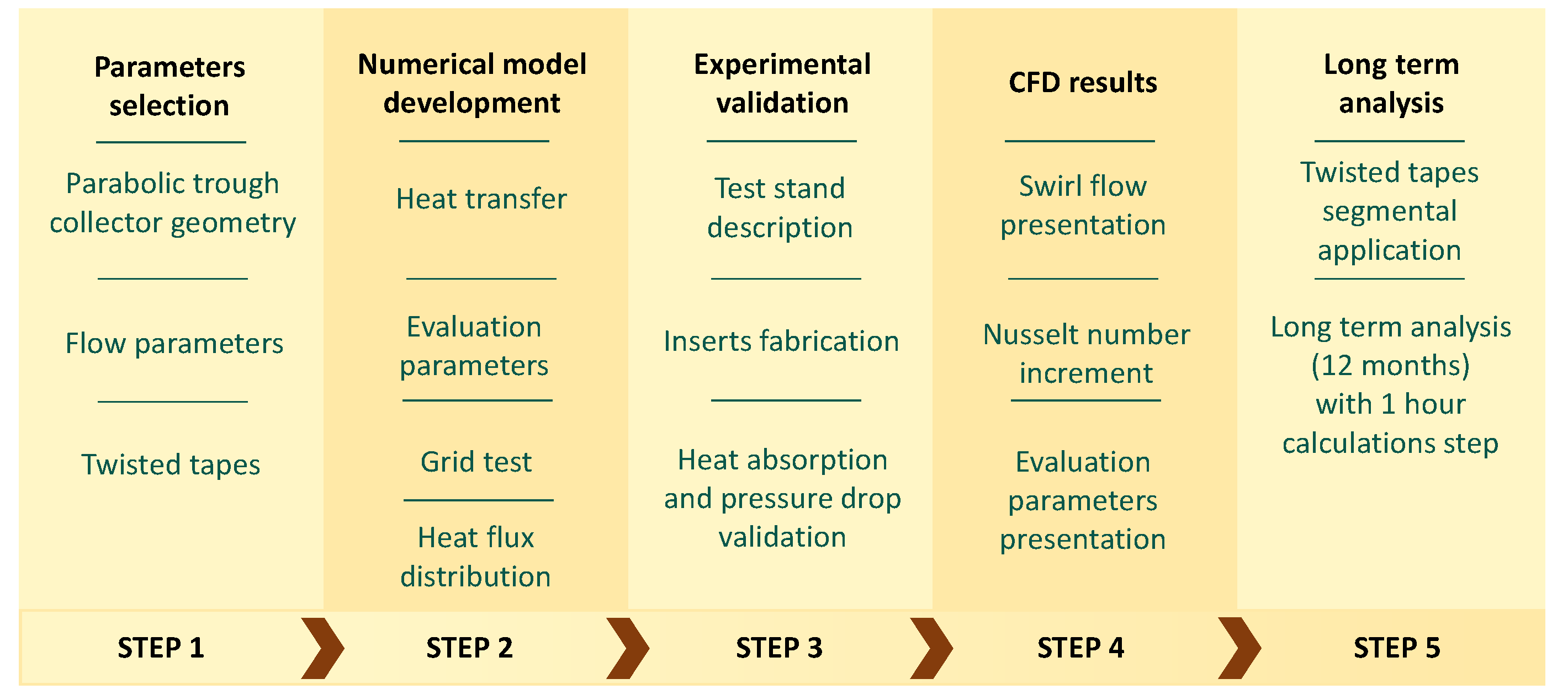
This article presents a strategy for a segmental application of flow turbulence inserts in a solar absorber loop for low-concentrated parabolic trough collectors. The use of twisted tapes with different twisted ratios is aimed at intensifying heat absorption while simultaneously searching for the solution that generates the smallest pressure drop. This research is divided into 5 steps, presented in
Figure 1.
The first step is to select the right geometrical parameters of analysed technology and flow parameters as well as twisted tapes. Second is the development of a parabolic trough numerical model. Third is numerical model validation. The next step is numerical results presentation and the last one is application of these results to a mathematical model to perform a long-term analysis.
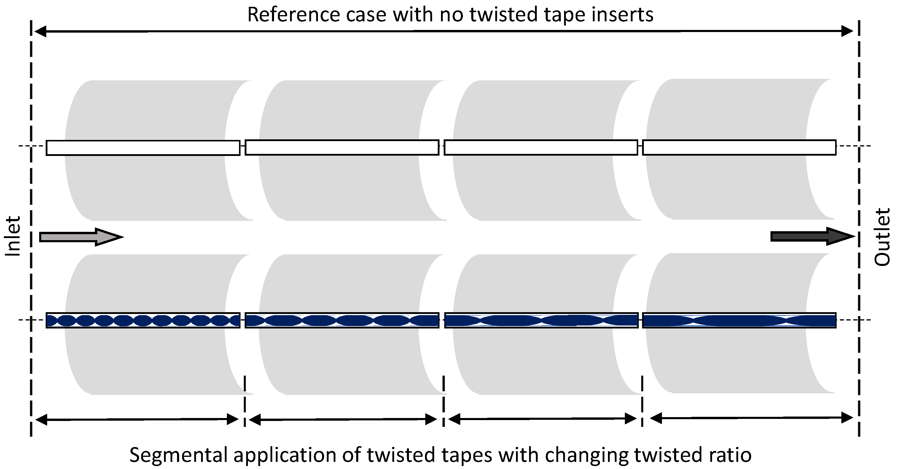
Figure 2 shows the potential application of turbulent inserts of different twisted ratios for particular segments of the absorber loop.
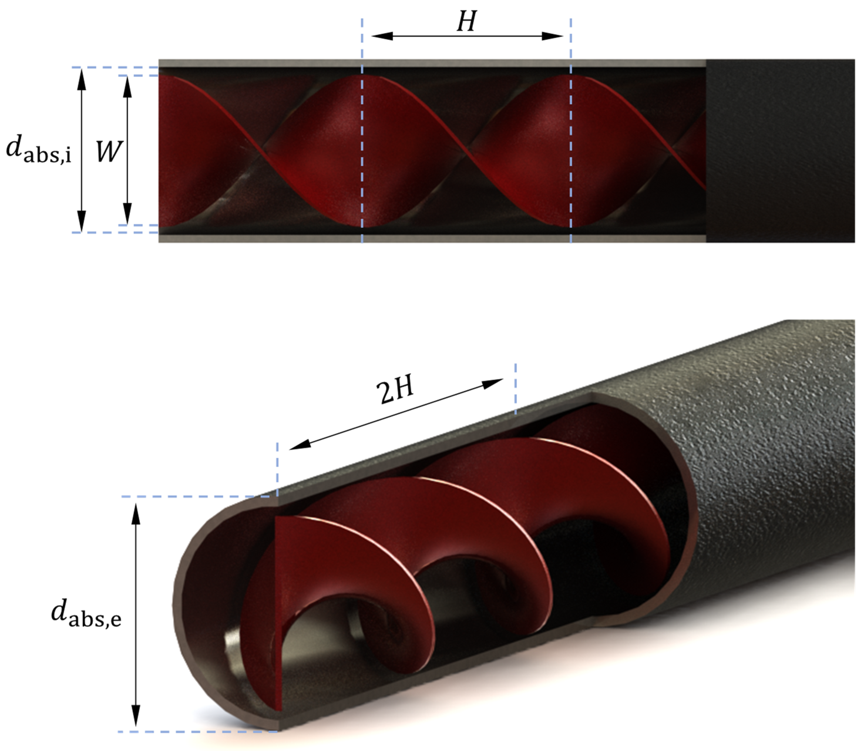
Twisted tapes are components made by twisting a flat strip, usually steel, causing a given number of turns per length. An illustrative visualisation of the twisted tape built into the linear absorber, along with the marking of the geometric characteristics, is shown in
Figure 3. A twisted ratio is defined as [
34]:
where
H is the length equivalent to 180° turn and
dabs,i is the internal diameter of the absorber. In the case studied, inserts with twisted ratios of 1, 2 and 4 were considered. Parameter 2
H defines the full rotation of the twisted tape insert. The second parameter that defines the insert is the width ratio, which is defined as [
35]:
where
W is the width of a twisted tape. One width ratio configuration of 0.9 was considered in this analysis. For each case, the thickness of the insert was 1 mm. For the purpose of the analysis, the insert was assumed to be placed directly on the axis of the absorber.
The analysis was performed for a parabolic trough collector; the geometric dimensions and optical parameters are summarised in
Table 1, which reflects the parameters of the PolyTrough 1800 [
36]. A linear absorber made of steel is surrounded by a glass envelope, with very low pressure close to the vacuum in between. The studies were conducted for three mass flow rates of 0.15 kg/s, 0.225 kg/s and 0.3 kg/s and five inlet temperatures of heat transfer fluid: 60 °C, 100 °C, 140 °C, 200 °C and 250 °C, which corresponds to a large percentage of installations with low-concentrated parabolic trough collectors [
12]. The radiation delivered to the absorber is described in detail later in this section. The parameters of the selective coating used for the analysis correspond to the TiC-TiN/Al
2O
3 coating [
37]. Therminol VP-1 was chosen as the heat transfer fluid. The selected fluid is an Eastman product, widely used in parabolic trough collector installations. The composition of the fluid is a eutectic biphenyl/diphenyl oxide mixture, where the operating temperature is 12–400 °C.
Table 2 shows the parameters of Therminol VP-1 as a function of its temperature, based on the manufacturer’s data [
38].
Later in this section, the heat flow in the parabolic trough collector is briefly described, compiling the main equations and evaluation parameters. The next section describes the numerical studies and the assumptions and boundary conditions. The long-term analysis presented in the article section uses a previously developed mathematical model. A detailed description of the model and its validation has been presented in previous analyses [
21].
2.1. Heat Transfer in Parabolic Trough Collector
The parabolic trough collector is a device that utilises solar direct radiation. The use of a tracking system to follow the sun during the operation period is required for proper operation [
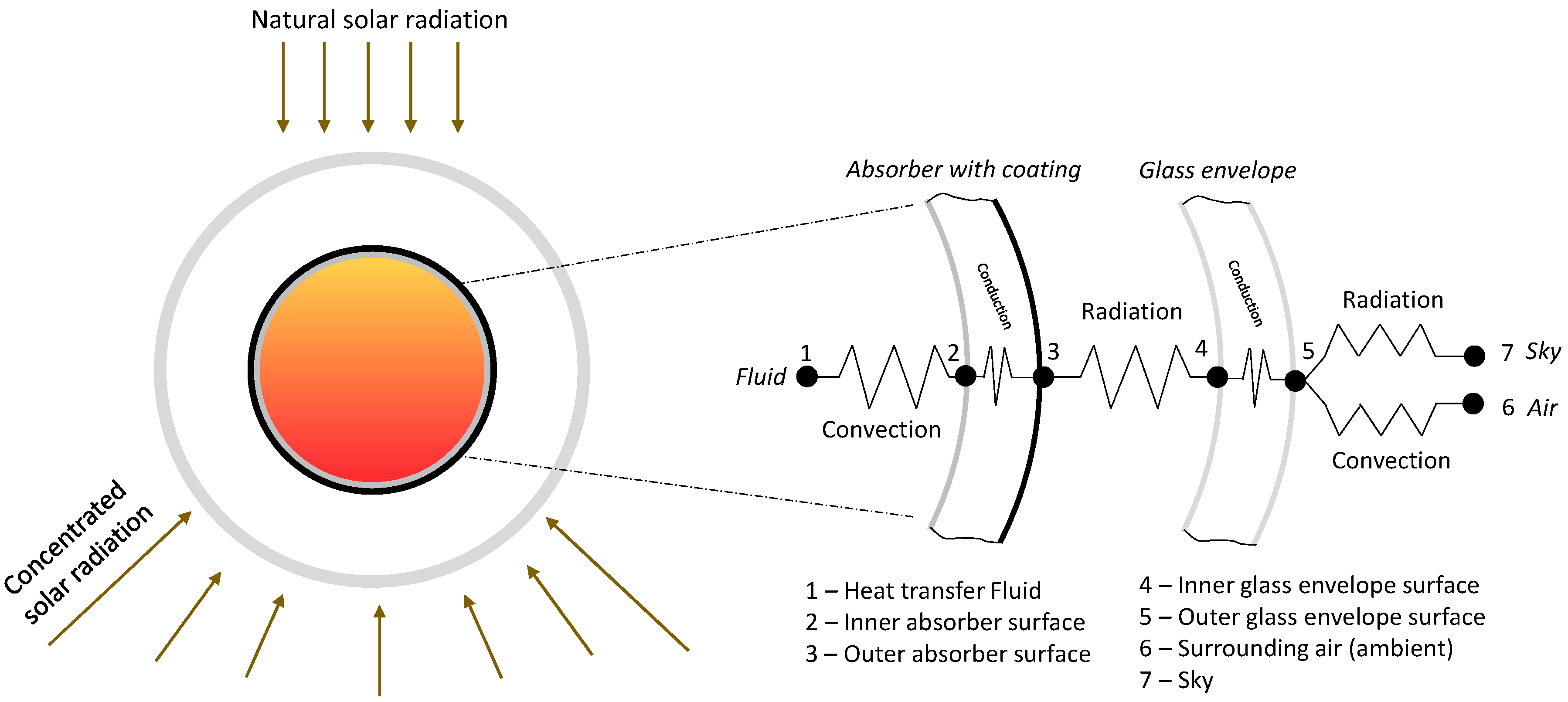
39]. Direct radiation is reflected from the parabolic shape mirror and concentrated on the outer surface of the absorber tube. A linear absorber with a circular cross-section is placed in the focus of the collector. Multiplied reflected radiation results in a non-uniform distribution of radiation on its outer surface. Radiation directly delivered to the external surface from the side facing the sun also reaches the absorber. In most cases, the heat delivered in this way represents a low proportion of the total power input. Still, when analysing parabolic low-concentration devices, this heat represents a noticeable proportion and must be considered. The heat flow model and thermal resistance for the receiver cross-section are shown in
Figure 4. Heat flow in the receiver assumes convection between the inner absorber wall and heat transfer fluid, conduction through the absorber, radiation loss between the external absorber surface and internal glass envelope surface, conduction through the glass envelope, convection loss between the external glass surface and ambient and radiation losses between the external glass envelope surface and sky. In the case studied an ideal vacuum was assumed between the external absorber surface and the glass envelope.
The following equations present the main heat flow correlations of the analysed installation. The useful heat absorbed by the thermal fluid is calculated as Equation (3) according to [
40]:
where
Qu is the useful thermal energy collected by heat transfer fluid,
is the mass flow of circulating fluid,
cp is the specific heat and
Tout −
Tin is the difference between outlet and inlet temperature.
The heat flux can be also presented as a difference between solar energy reaching the absorber and heat losses (convection and radiation) [
41].
where
Aap is the aperture surface area,
dabs,e is the absorber external diameter,
GB is the direct solar irradiance,
ηopt,CSP is the optical efficiency for CSP, θ is the incident angle, IAM is the incidence angle modifier,
L is absorber length and
ηopt,SP is the optical efficiency for solar power. The equation was used as a boundary condition in a CFD simulation in the twisted tape area.
This approach separates the concentrated and non-concentrated radiation that is delivered to the absorber surface. The optical efficiency is therefore divided into two parts, relating to the corresponding path through which the radiation passes on its way from the sun to the absorber surface. A full description of our proposed model, detailing the individual components, has been presented in our previous publications and, to maintain the conciseness of the results from that study, is not repeated here [
21].
Total solar energy received by a PTC installation is defined as Equation (5) [
42]:
The efficiency of the parabolic trough should consider both the heat absorbed by the linear absorber and the power required to drive the heat transfer fluid pump. For this purpose, Equation (6) was presented as follows [
25,
43]:
where
ηPTC is parabolic trough collector efficiency,
Wp is the required pump power and
ηel is the reference electricity production efficiency. For purposes of this analysis, the value 32.7% is selected [
44].
The pumping work demand for the fluid movement is calculated as [
25]:
where Δ
P is pressure drop and
ρ is the density of fluid.
The pressure drop can be calculated using the friction factor and Darcy–Weisbach equation:
where
f is friction factor and
u is fluid velocity.
For smooth absorber the value of friction factor can be used by Petukhov’s correlation [
45]:
The average Nusselt number is given according to Gnielinski’s correlation, which is valid for low and high Reynolds numbers [
46]:
where
Pr is Prandtl number.
For evaluation of thermal performance at constant pumping,
PEC (performance evaluation criterion) coefficient was used [
47]:
PEC index is a flow criterion which evaluates the heat transfer coefficient enhancement increase under the equivalent conditions of same pumping work demand.
2.2. CFD Model
Numerical calculations were performed with Ansys Fluent 19.2 using a discretised 3D domain [
48]. In the case of a PTC with a twisted tape, it is not possible to apply domain optimisation techniques using, for example, the AxiSymmetric 2D feature, due to the non-axisymmetric design of the studied structure. The research was performed at a steady state and turbulent flow is modelled by the Reynold averaged Navier–Stokes (RANS) equations [
49]. A pressure-based solver was used, and the governing equations of mass (12) and momentum (13) were defined as follows [
50]:
where
is the effective viscosity defined as the sum of the molecular viscosity
and the turbulent viscosity
according to the formula:
CFD (computational fluid dynamics) calculations are carried out in the fluid region of the absorber, in which there is forced fluid flow between the inlet and outlet boundaries at a given mass flow rate and inlet temperature. The process of heating the fluid occurs as a result of the external heat flux, the value of which depends on the position of the wall point (x,y) in the plane normal to the inlet plane. The heat flux was implemented using the User Defined Function (UDF) [
51]. The twisted tape along the entire length of the absorber is an area inert to the flowing fluid and is not involved in any heat transfer process. The energy conservation equation is defined as:
Cabello et al. [
52] performed an extensive analysis of different turbulence models and their impact on modelling flow and heat transfer in a PTC with a twisted tape. The authors showed that the accuracy of individual turbulence models varies with the values of Reynolds (
Re) and Twisted ratio (
Tr). They also proved that the k-ω SST model simulates the desired phenomena with high accuracy in the range of
Re > 17,000 and
Tr ≤ 4. Due to the study of
Tr in the range of ≤4 and the expected relatively high ranges of the
Re number, it was decided within the scope of this article that the k-ω SST turbulence model would be used [
53]. The basic equations for turbulence kinetic energy
and specific rate of dissipation
are defined according to relations (15) and (16) [
54,
55]:
The inlet boundary condition included the mass flux of the Therminol and its temperature. The mass flux
is expressed by the formula:
where
is the inlet cross-sectional area. Therminol parameters were calculated from the material data shown in
Table 2, which were implemented into the numerical model. The flux and inlet temperature variables for the validation of the numerical model with experimental data were implemented as external data arrays.
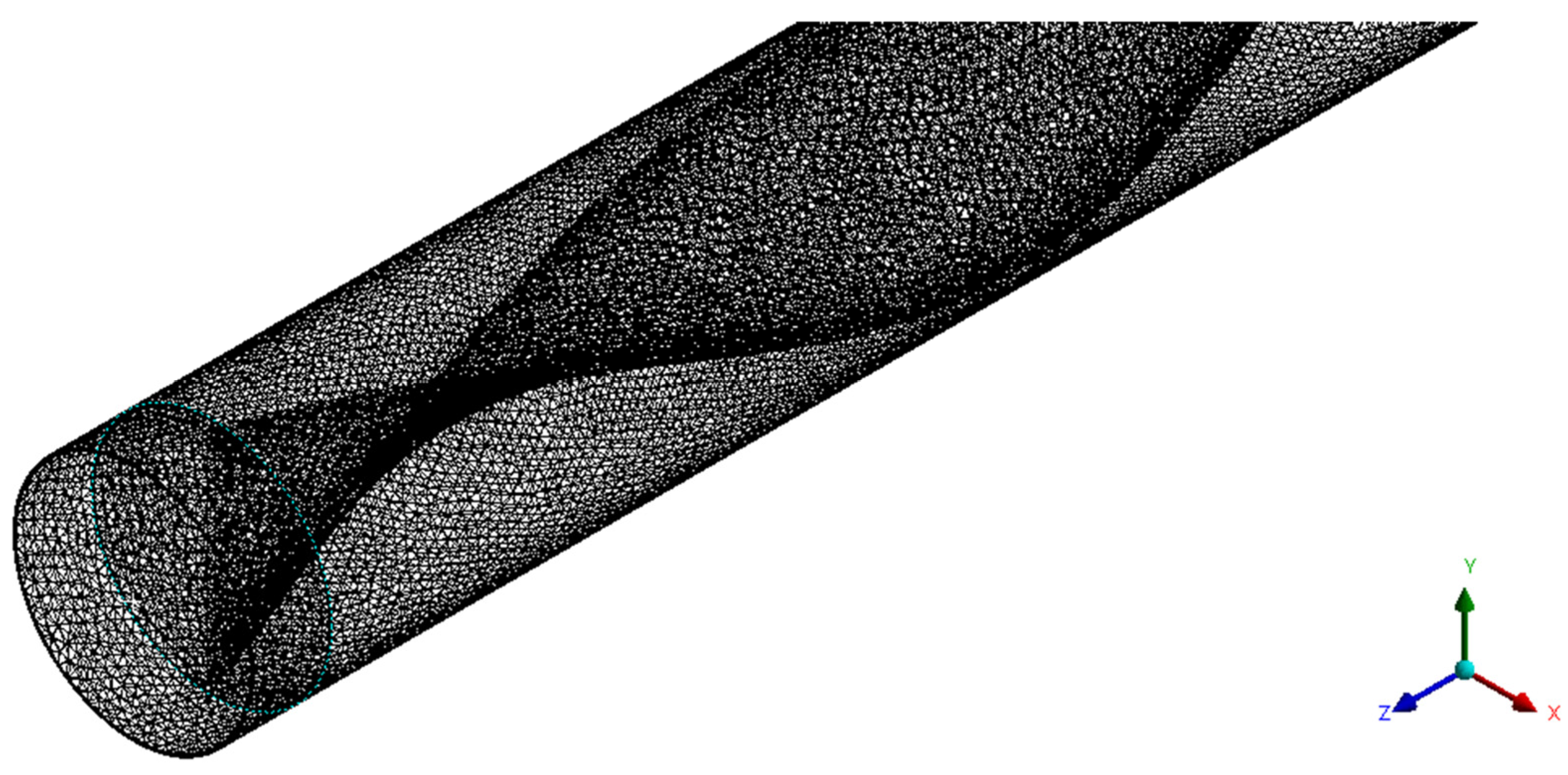
The computational domain was divided into subareas to optimise the numerical grid. The sub-area covering the occurrence of a twisted tape was covered by additional compaction of the elements of the numerical grid, especially around the edges of the tape. An inflation layer was generated along the entire length of the numerical model. In addition, the inlet area in front of the twisted tape was modelled to achieve fully developed fluid flow. This area was not subject to the presence of an external heat flux applied to the external surface of the model. An example of a numerical grid is presented in
Figure 5.
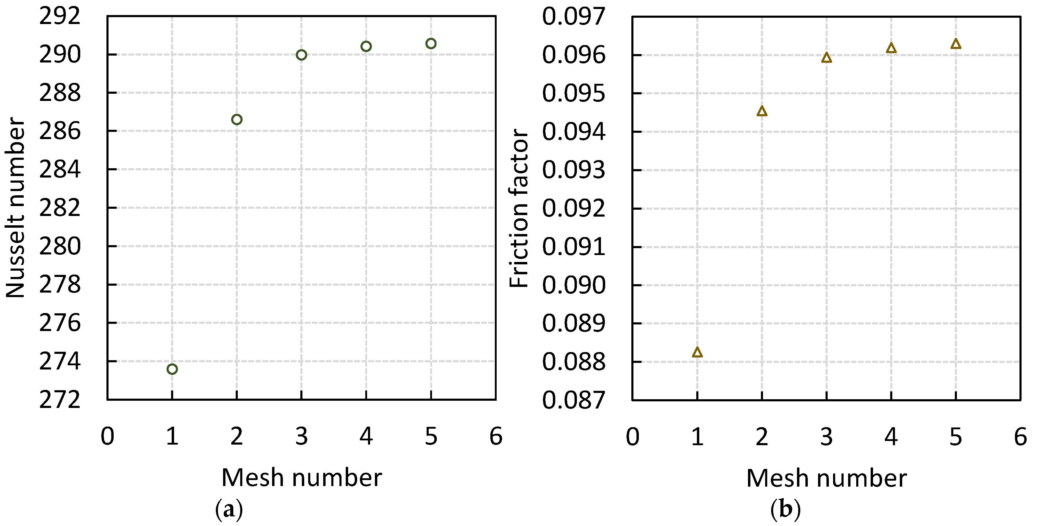
A grid independence test was performed, during which the degree of influence of the quality of the numerical grid on the results obtained was investigated.
Table 3 presents the details of the studied numerical grids.
Figure 6 shows a comparison of the results of PTC parameter calculations with a twisted tape for different numerical grids under the same boundary conditions. The values of the Nusselt number and friction factor were determined using Equations (8) and (9).
It was shown that, as the number of elements and nodes of the numerical grid increases, there is an asymptotic increase in the values of the calculated parameters. The largest deviation from the limit of the result was recorded for grid 1 (about 6% for
Nu values). Between grids 3 and 5 there were no significant differences in the results, with a difference of about 0.2% for the
Nu value. Both the residuals and the parameters monitored during the calculation were taken as the convergence criterion. The moment when the difference between successive results of the average temperature of the fluid at the outlet did not exceed a specific value was taken as the steady state. The same range of values is applied to the parameter of pressure drop along the length of the twisted tape in the absorber. As the number of numerical grid elements increased, the time to achieve the expected convergence of steady-state calculations noticeably increased. Therefore, it was decided that grid number 4 was optimal in terms of the accuracy of the results obtained and the time required to carry out a single series of calculations. The selected numerical grid has an average skewness value of about 0.21 with a maximum skewness not exceeding 0.5, indicating the very good quality of the numerical grid elements providing satisfactory accuracy of numerical calculations. The inflation layer cell of this mesh has a height of 0.05 mm (with a maximum of 10 inflation layer elements), and the value of the y+ parameter is ~1.6, which is the respected value for the turbulent flow model used [
56]. The numerical grid was used at the stage of validation of the mathematical model with experimental data.
The heat flux supplied to the linear circular absorber was determined using the optical-engineering software APEX [
57]. This numerical software allows tracking of the simulated rays and analysis of the illuminated surface, considering the individual components of the system and their optical properties [
58]. The software enables the calculation of the radiation distribution and power analysis of a selected surface, including parameters such as shape, reflectivity, absorptivity, surface roughness and coating. The software adopts a Monte Carlo ray tracing method [
59,
60]. The tool was selected based on its commercial maturity, cooperation with Solid Works software and satisfactory accuracy. The selected ray tracing method is also frequently used in the modelling of solar radiation simulators [
61,
62,
63]. In the MCRT method, the Bidirectional Reflectance Distribution Function (
BRDF) is used to describe the reflected beam behaviour [
64]. This method tracks the energy of each simulated ray and calculates the total flux as well as its distribution. The
BRDF describes the form in which light incident on a given surface is scattered. The BRDF function is defined as the scattered radiance per unit incident irradiance and is described by Equation (19) [
65].
where
is the unit of radiant energy per unit of solid angle (W/m
2sr); the irradiance
is the incident power flux density per unit area (W/m
2). The angles
are the polar and azimuth incident angles and polar and azimuth reflected angles, respectively.
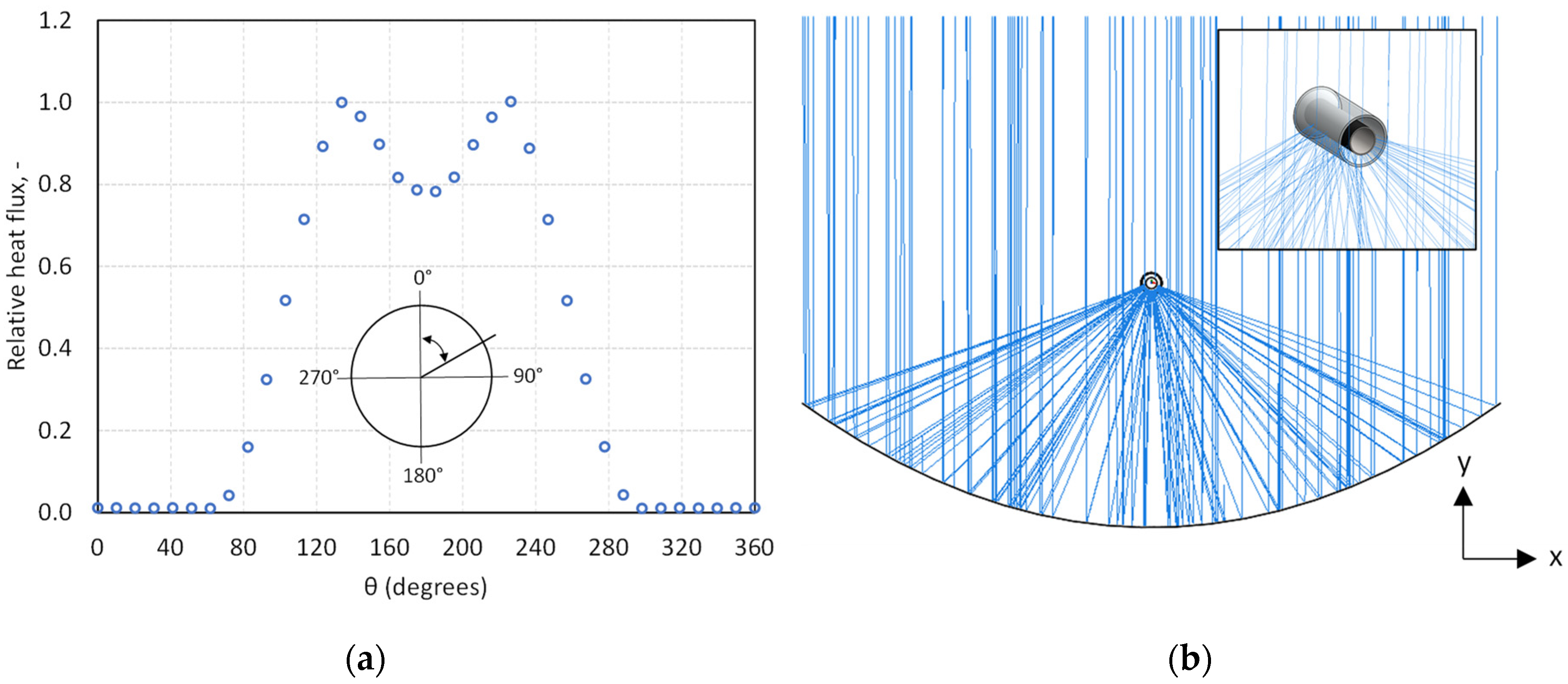
A numerical model of the respective solution is shown in
Figure 7. The model includes a parabolic mirror with assumed reflectivity, a tubular absorber made of steel and coated with a selective coating, and a glass envelope with given transmittance. The calculations were performed by modelling direct normal radiation. Sun model was used as a radiation source, which included the solar half angle
θs = 0.27°.
Figure 7a shows the radiation distribution on the outer surface of the absorber, along with the marked angle used in previously mentioned UDF. The radiation distribution is an input to the numerical model.
Figure 7b shows the simulated rays and their reflection from the surface of the parabolic shape mirror. Rays number used in each model was 2·10
8 which provided highly accurate results which were presented in the previous publication [
16].
3. Results and Discussion
3.1. Model Validation with Experimental Research
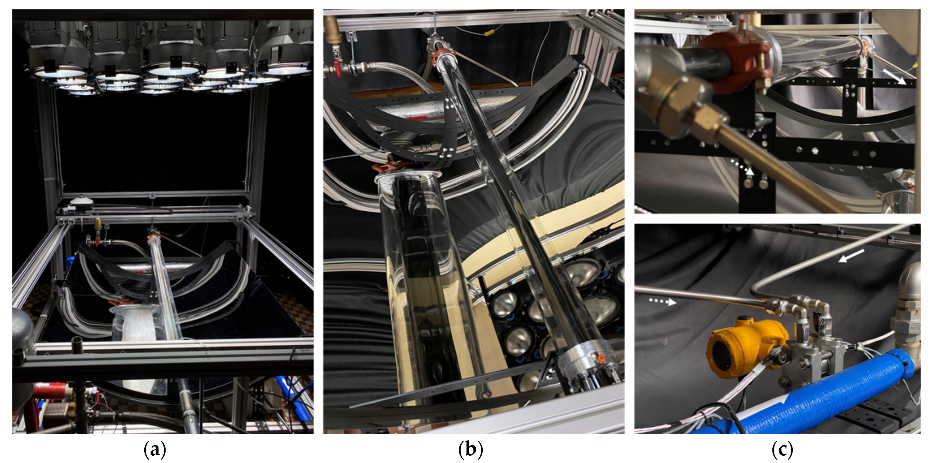
Validation of the numerical model was carried out using the laboratory test stand shown in
Figure 8. The bench consists of two main components, a solar radiation simulator and a parabolic trough collector [
66]. The simulator consists of 18 metal halide lamps (HMI), 575 W each, with the possibility of reducing the power to 60% of the nominal value. The variable distance of the light source from the reflector allows for a changing character of radiation, from diffuse to direct. Furthermore, lenses are fitted to the reflectors to collimate the radiation to ensure that the rays are as similar to natural radiation. The system is air-cooled so that the impact of heat from the source on the ambient temperature can be reduced. The construction of the solar radiation simulator stand was preceded by a series of numerical analyses, based on the Monte Carlo ray tracing method and optimisation of their location [
61,
67]. The optical numerical model was experimentally validated and the results indicated high agreement.
The second component of the stand is a parabolic trough collector with a low concentration ratio. It consists of a parabolic mirror and a linear absorber located at its focal length, which is presented in
Figure 8b. The mirror with an aperture of 1 m and a length of 1 m is made of highly reflective sheet metal. The linear absorber, with an external diameter of 33.7 mm, is made of mild steel and coated with the highly-absorptive Pyromark coating, often used in various solar installations [
68]. The absorber is located in a glass envelope made of borosilicate glass and connected by two brackets, at the beginning and the end of the absorber. A low pressure, close to vacuum, is maintained between the steel tube and the glass envelope to reduce heat loss. The value of the simulated radiation is measured using a pyranometer and a heat flux meter (at the focus of the parabolic mirror). The heat-transfer medium is Therminol VP-1. The quantities measured on the solar loop side are the temperature increment with K-type thermocouples, the volumetric flow and the pressure by the differential pressure sensor, shown in
Figure 8c, which is crucial in assessing the use of turbulence inserts as it measures the pressure drop in the absorber pipe.
For experimental validation, tests were carried out for three cases. The first one was for the plane absorber, the second for the absorber with twisted tape where the twisted ratio was 7.6 and the third was for the absorber and twisted tape with a twisted ratio 3.8. The twisted tapes inserts were fabricated using 3D printing technology, from a PETG (polyethylene terephthalate glycol) material that had previously been selected from many others as the most durable for Therminol VP-1. However, it needs to be noted that inserts made of this material cannot be used in long-term analyses or for industrial applications. It is necessary to manufacture them in steel, but at this stage of the analysis, 3D printing, characterised by high accuracy, was used to perform fundamental tests. The inserts were printed in sections of 190 mm and then joined on a 4 mm diameter threaded rod to keep the insert stable. The total length of the twisted tape was 950 mm. Then, with the support of appropriate adapters, the insert was placed inside the absorber in such a way that it was positioned as close to the centreline as possible. The analysed inserts are shown in
Figure 9.
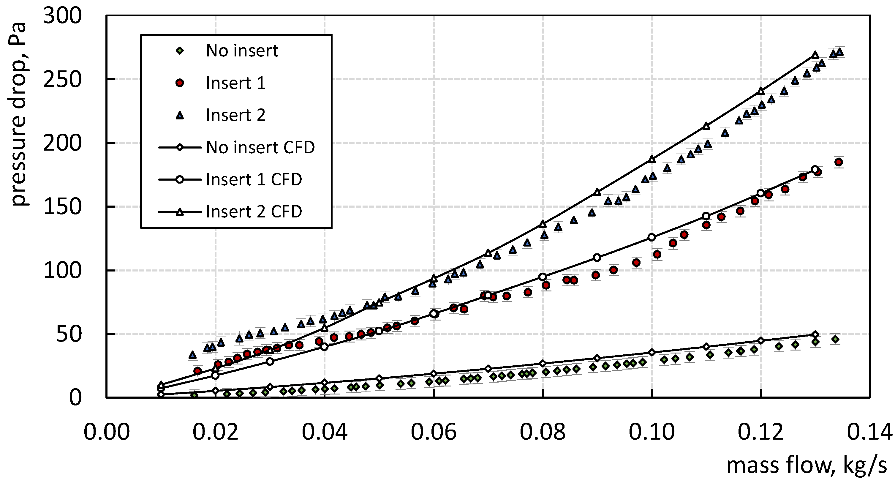
Following an analogy with other studies using CFD presented in this article, models were made based on the geometry of the inserts used for the experimental analysis. The first parameter validated was the pressure drop as a function of flow. The pressure drop was measured using an Aplisens APR-2000 ALW (Aplisens S.A., Katowice, Poland) pressure drop sensor with a base error of 0.075% and a base range of −2.5 kPa–2.5 kPa. A Kobold DON-215HR33H0M0 (KOBOLD Instruments, Warsaw, Poland) flow meter sensor with accuracy reported by the manufacturer 1% was used for flow measurement. The results are shown in
Figure 10, where the pressure drop for the three cases is presented as a function of mass flow, determined from the volume flow from the flow meter and temperature. For all cases, the tests were carried out at constant temperatures and with the radiation simulator off. The same boundary conditions were maintained for the CFD study. Experimental measurements were made for each point separately, where a series of measurements were carried out for stable conditions. Based on the accuracy of the measuring devices, a measurement uncertainty analysis was carried out for each measurement. A-type and B-type uncertainties were determined, as well as the compound uncertainty according to the guide uncertainty measurement (GUM) [
69]. The results are shown as uncertainty bars in
Figure 10.
The results obtained show a high correlation and agreement between the numerical model and the experimental tests. Despite some deviations from the curve obtained in the CFD studies, it should be noted that the shapes of the curves are consistent with the characteristics obtained in the measurement. In the numerical model, the tube joints and impulse pipe connections that occur in the actual stand were not considered. In addition, during the tests, air bubbles may have appeared in the actual bench which could have disturbed the measurement. Another factor affecting the differential pressure sensor was the vibrations accompanying the pump operation. It was noted that, for higher flows, the differential pressure sensor reacted to the vibrations accompanying the stand.
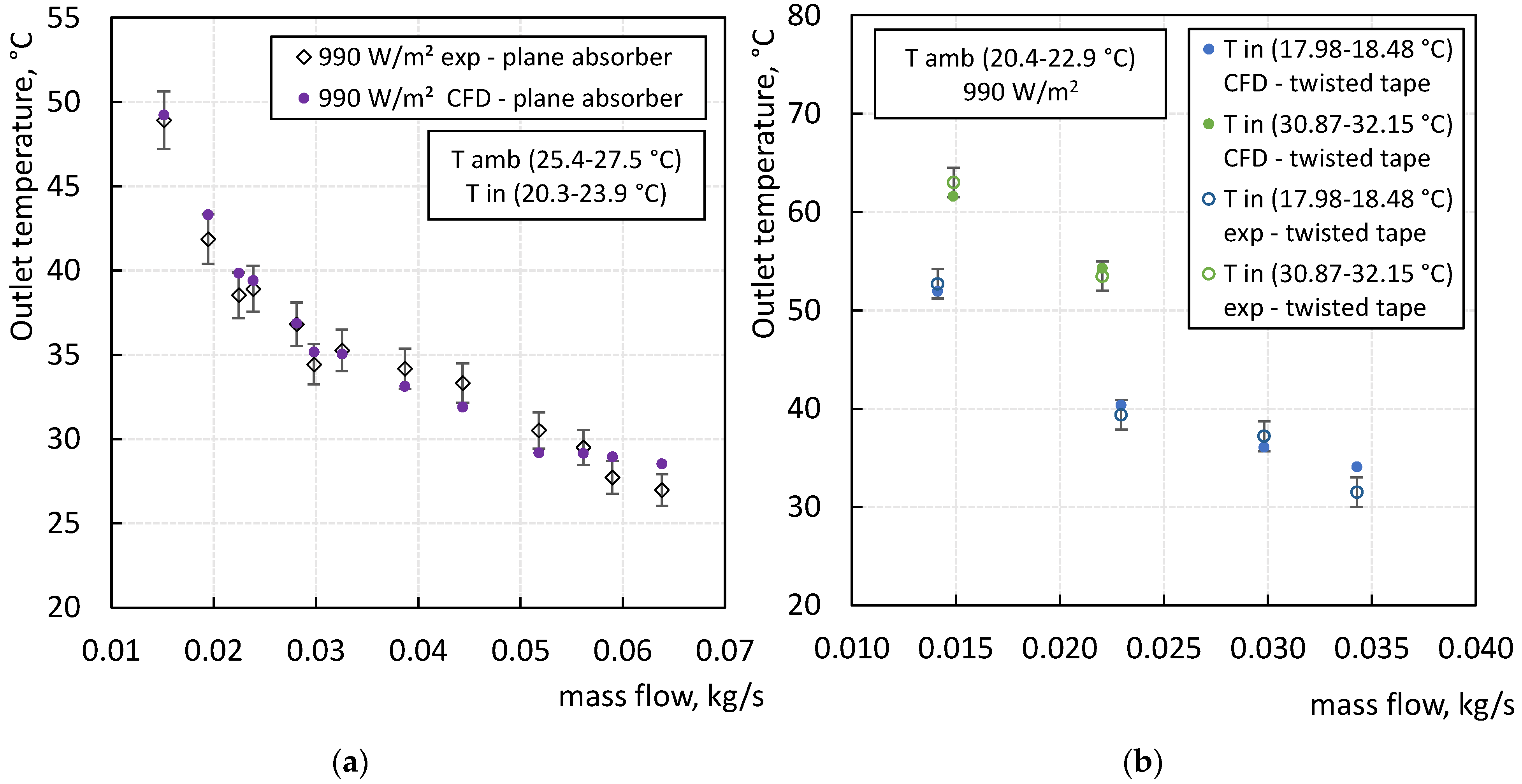
Validation of the temperature increase of the heat transfer fluid and thus the efficiency of the absorber is shown in
Figure 11. Tests were carried out in two cases: (a) where an absorber without inserts was analysed and (b) an absorber with insert with Tr = 3.8. The resulting temperature values were read for steady state and each measurement point marked in chart is the average of at least 200 measurement points. For each case analysed, there is a corresponding ambient temperature value and an inlet temperature that varied slightly. For each measured point on the experimental bench, tests were carried out using CFD for the same boundary conditions parameters. The plotting of points on the graph highlights the high accuracy of the model.
Based on the results presented, it can be concluded that the CFD model made represents the actual installation parameters well and can be used for testing twisted tapes.
3.2. CFD Analysis Results
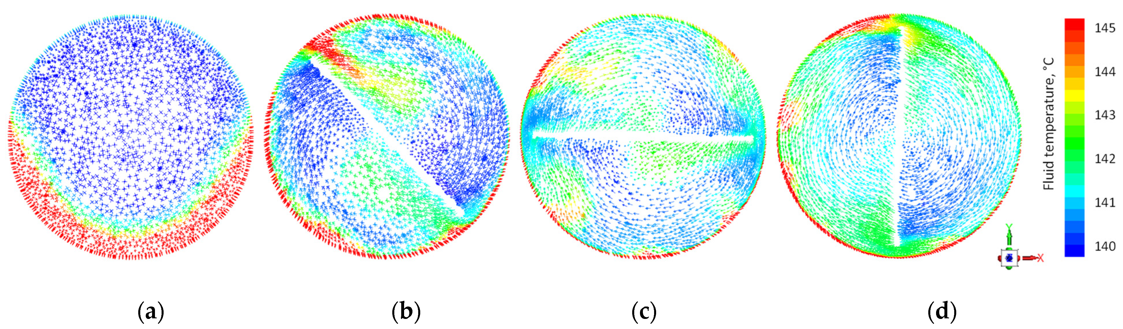
Figure 12 presents mass flow vectors coloured by fluid temperature for four cases in equal absorber cross sections. For each, the boundary conditions are the same but differ in the twisted ratio. The figures represent the reference case without a turbulent insert (a) and three inserts with twisted ratios of 4, 2 and 1, respectively (b), (c) and (d). It can be noted that the flow vectors in the reference case are directed perpendicular to the absorber cross-section. In contrast to this case, for the inserts used, the nature of the flow changes and the vectors show fluid circulation around the absorber axis. For the reference case, it is noticeable that there is a significant non-uniform temperature distribution in the absorber due to the heat flux distribution on the absorber surface, which causes a large temperature difference and can affect material stresses and reduce durability. The swirl flow, caused by the twisted tapes, significantly reduces the temperature difference in the absorber and mixes the fluid, improving the heat transfer conditions and reducing boundary layer thickness. A noticeable trend is that the smaller the twisted ratio, i.e., the tighter the insert, the more the temperature difference in the fluid decreases.
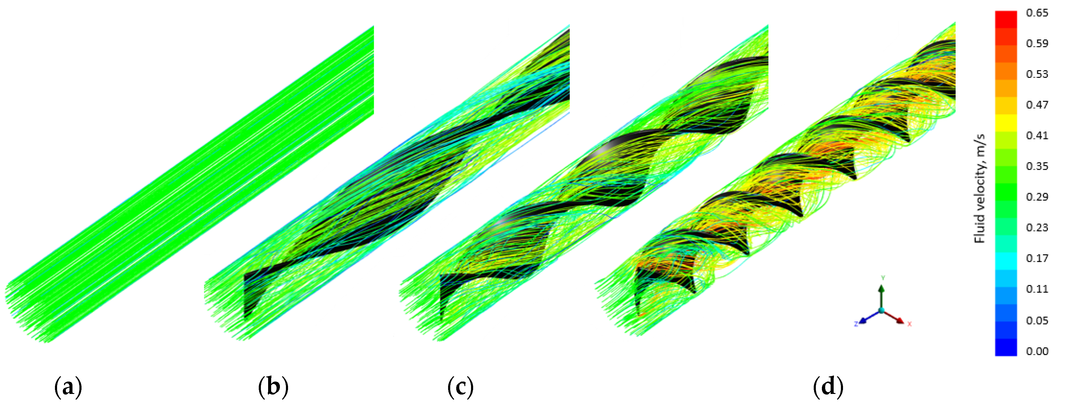
The use of twisted tapes has a significant effect on increasing the fluid velocity in the absorber, resulting in an increase in the Reynolds number.
Figure 13 shows the fluid path lines coloured by heat transfer fluid velocity. Twisted tapes cause swirl flow and extend the path of the stream in the absorber. As the twisted ratio decreases, the fluid velocity increases, which has its maximum closer to the axis of the absorber. Intense mixing of the fluid also occurs, which reduces local temperature maxima and improves heat collection.
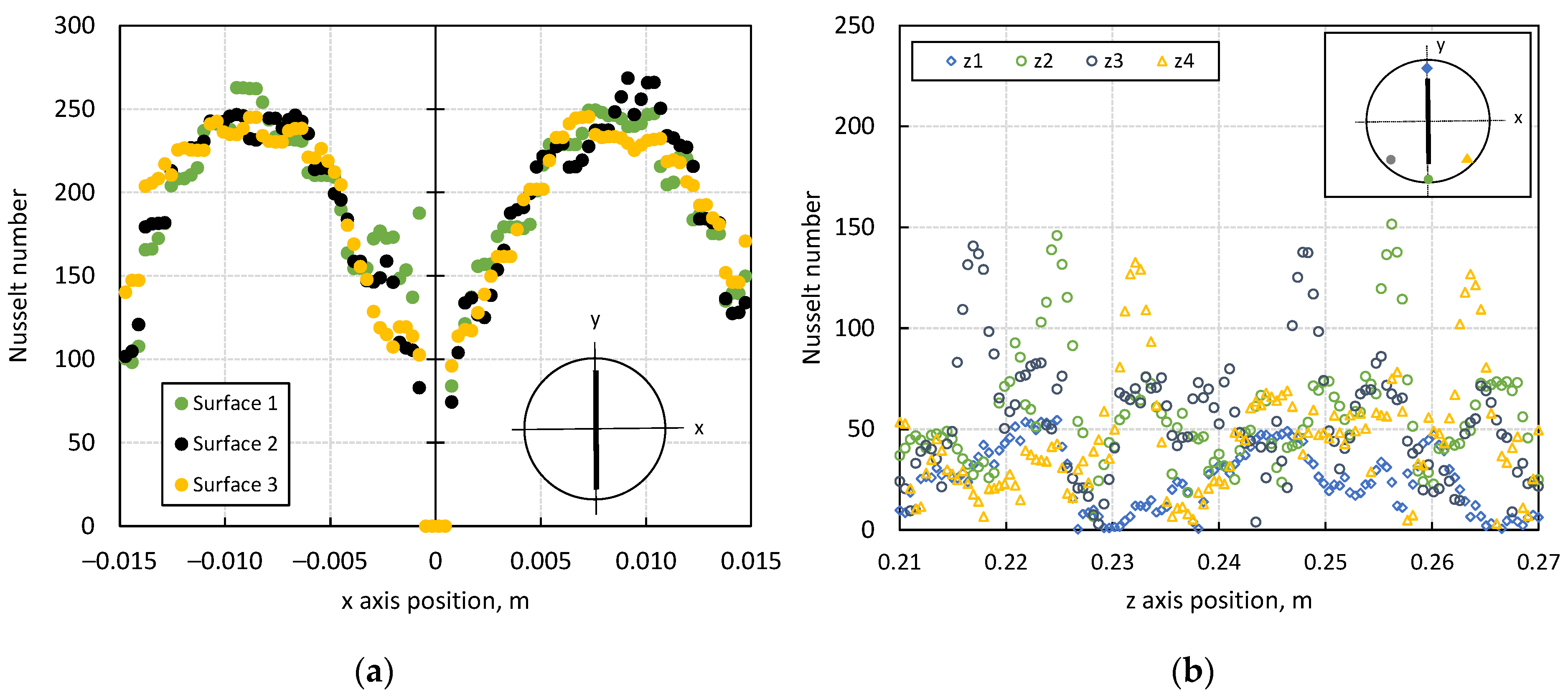
Figure 14 illustrates an example distribution of the local Nusselt number depending on the position in the absorber tube cross-section and along its length at selected points for Tr = 1. The results of the numerical analysis indicate a large variation in the local Nusselt number which is due to the nature of the flow, the previously demonstrated velocity difference and the non-uniform distribution of radiation on the outer surface of the absorber.
Figure 14a compiles the local Nusselt number for three selected cross-sectional areas, where the maximum appears in the areas between the insert and the inner wall of the absorber. The minimum can be identified closest to the twisted tape surface due to the low speed.
Figure 14b plots the local Nusselt number as a function of the length of the absorber and presents the results for 4 Z-axes, where Z1 is the axis closest to the upper surface and Z2, Z3 and Z4 occur closer to the surface with concentrated heat flux. For a given axis, the maximum of the Nusselt number can be identified where the twisted tape is close to the absorber wall, which is where the most intense heat extraction occurs. The lowest heat transfer occurs at the Z1 axis, which is close to the wall on whose surface the lowest heat flux is applied. Furthermore, comparing the local Nusselt number for the Z3 and Z4 axes, there is a lack of symmetry, which is caused by the particular direction of the fluid flow in the absorber pipe, the twisted tape being twisted to the right. Therefore, as can also be seen in
Figure 12, the heat absorption is higher on one side.
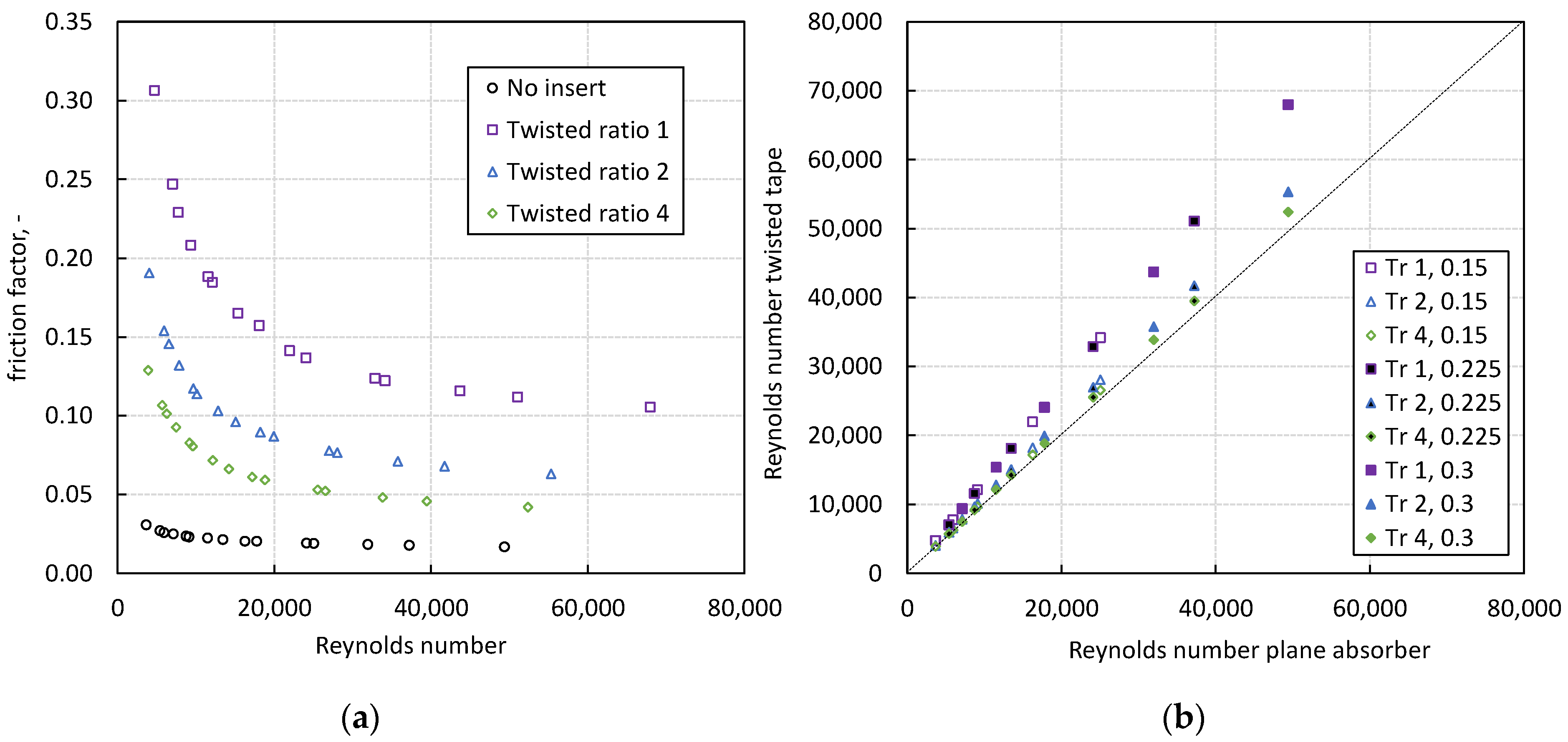
The placement of twisted tapes inside the absorber increases the fluid velocity, resulting in improved heat extraction conditions on the one hand and increased friction and pressure drop on the other. The pressure drop generated in the system forces the circulating heat transfer fluid pump to a higher power level and this reduces the efficiency of the system.
Figure 15a presents the friction factor for the reference case and different twisted tapes, as a function of the Reynolds number. An increase in this factor occurs for smaller Reynolds numbers and denser twisted tapes. For each case, the most significant decrease in friction factor occurs through turbulisation of the flow. The curves shown in
Figure 15a for the individual inserts indicate a significant increase in flow resistance with a lower twisted ratio. The increase in Reynolds number relative to the reference case is shown in
Figure 15b, where the Reynolds number for its equivalent for the plane absorber is compared for each twisted tape case analysed. The greatest increase is noticeable for denser inserts and higher flow parameters (higher mass flow and higher medium temperature).
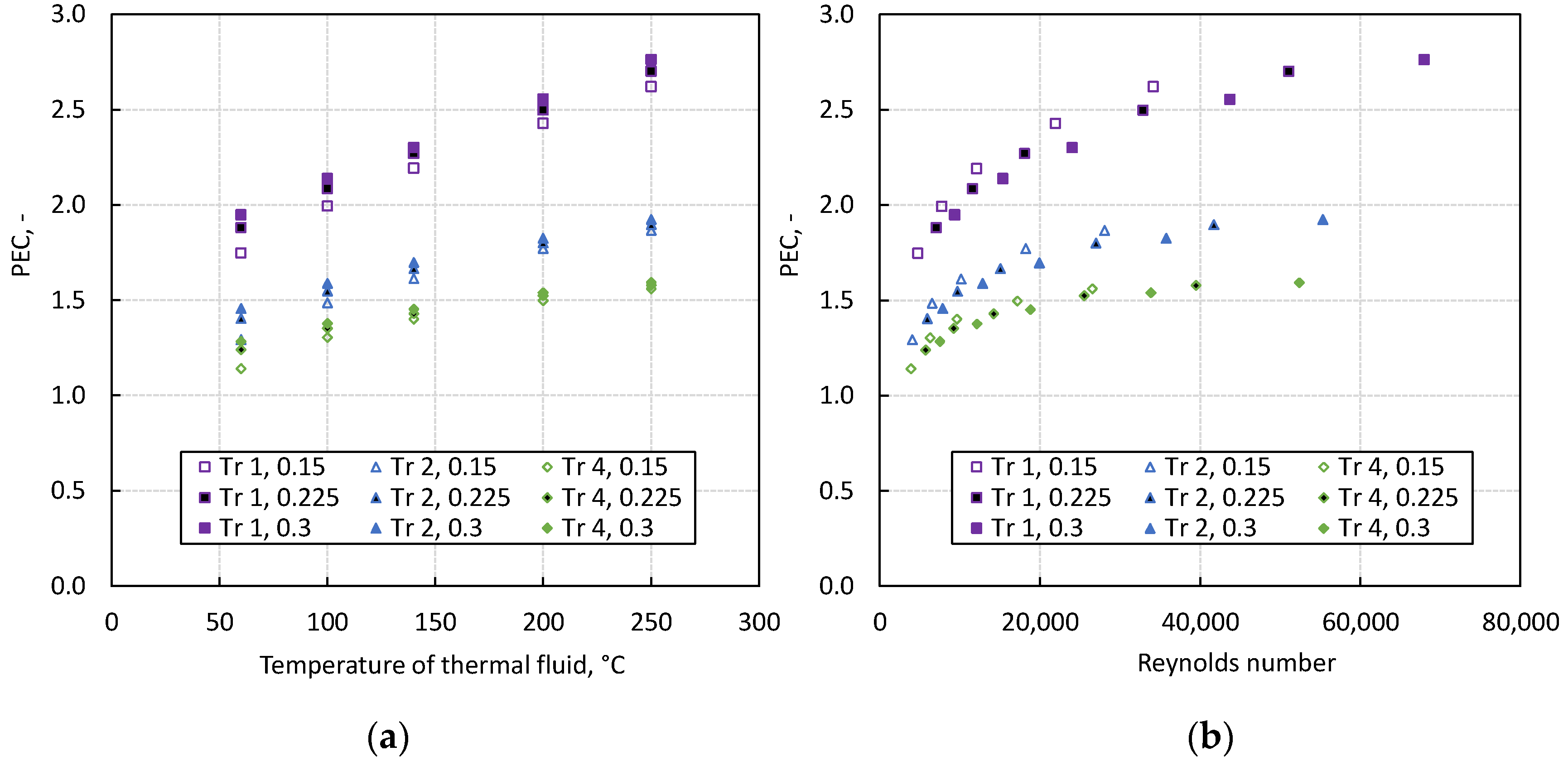
The PEC indicator shows heat transfer enhancement if its value is greater than 1. For the analysed data set, i.e., mass flow, temperature range and twisted ratio, a positive trend in PEC growth is maintained in each case, indicating that each analysed insert results in an intensification of heat absorption by the fluid. When considering the PEC index as a function of temperature, the greatest increase occurs for the highest mass flow and inserts with a low twisted ratio. When considering the PEC index shown in
Figure 16b as a function of the Reynolds number corresponding to the flow from the twisted tape, it can be seen that the given characteristic flattens out from a certain Reynolds number value. However, the most intense growth can be indicated for the range up to a Reynolds number of around 20,000.
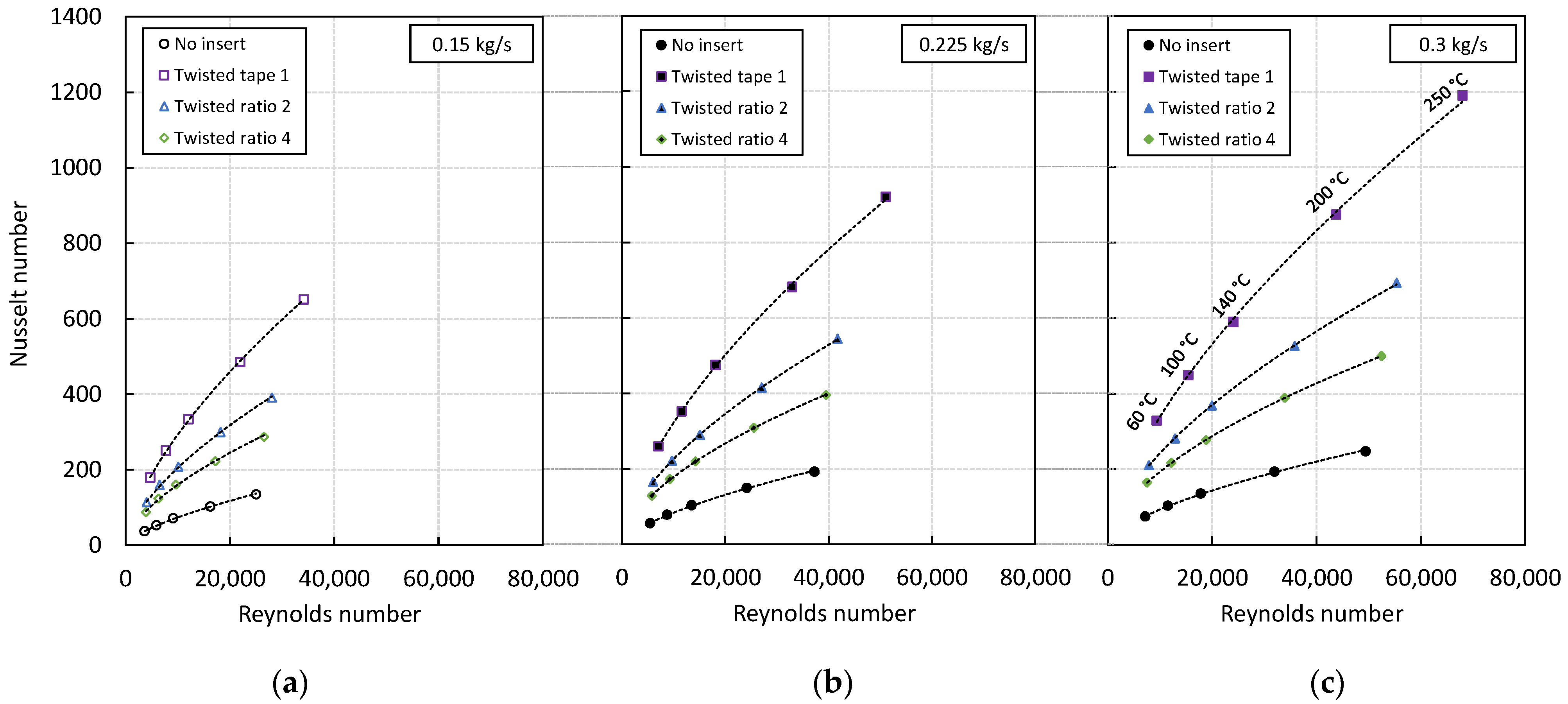
The average value of the Nusselt number as a function of the Reynolds number, for three mass flow scenarios and different absorber cases, with and without twisted tapes, is shown in
Figure 17. The Nusselt number increases with an increase in the Reynolds number, which in this case is due to an increase in fluid temperature, an increase in mass flow and twisted tapes with lower twisted ratios. That emphasises the intensification of heat extraction for the entire range of boundary conditions analysed. On each characteristic, each successive point is defined by an inlet temperature, successively 60 °C, 100 °C, 140 °C, 200 °C and 250 °C. It can be seen that with twisted tapes, the Reynolds number increases for each of the corresponding points due to the increase in velocity in the absorber. The largest increase occurs for an insert with a twisted ratio of 1.
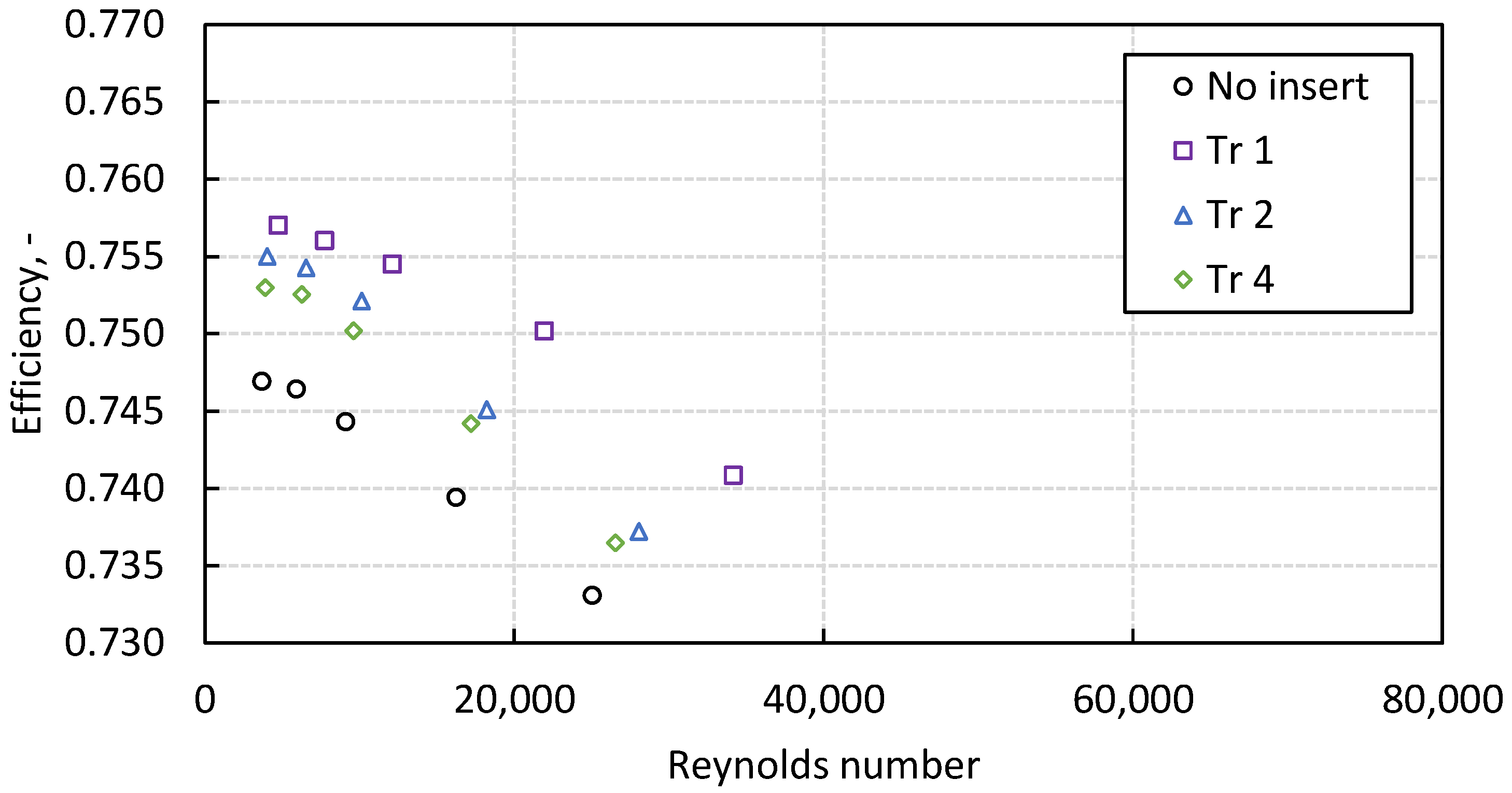
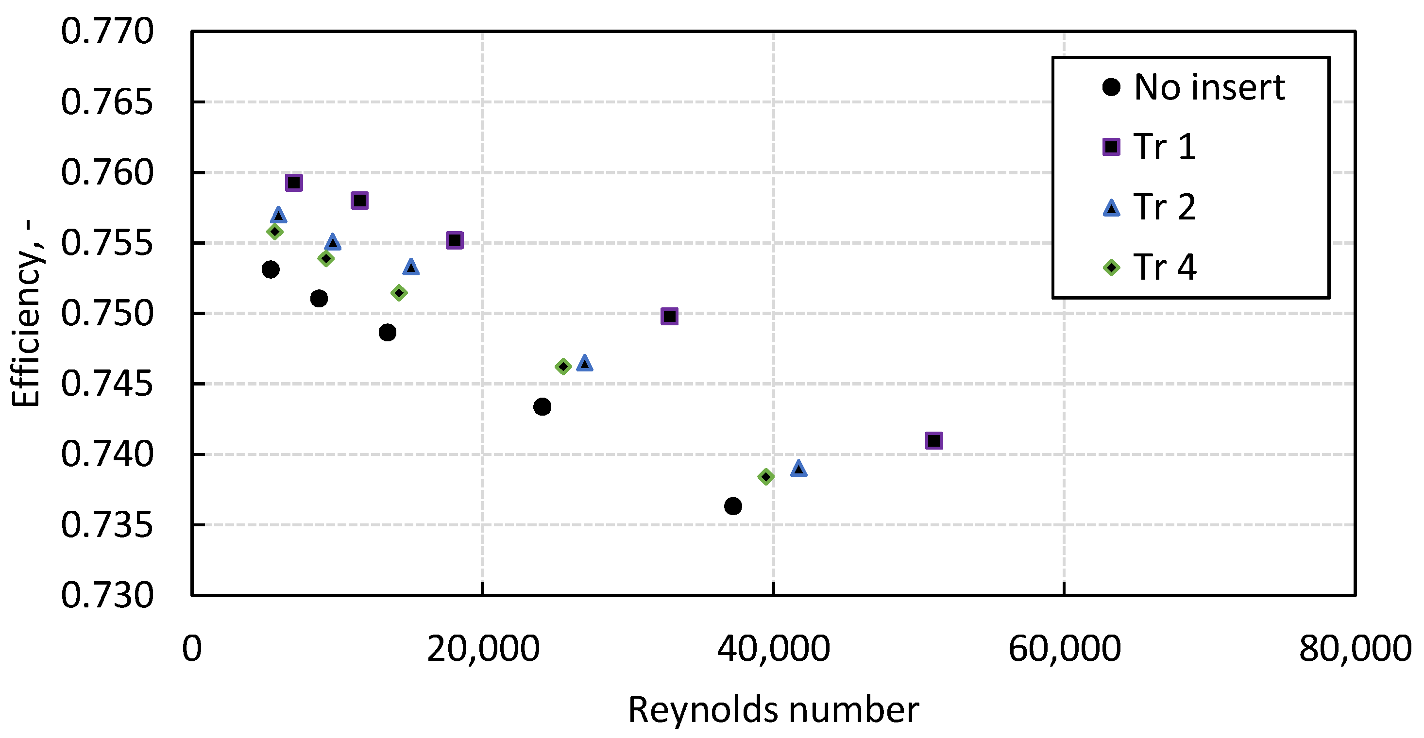
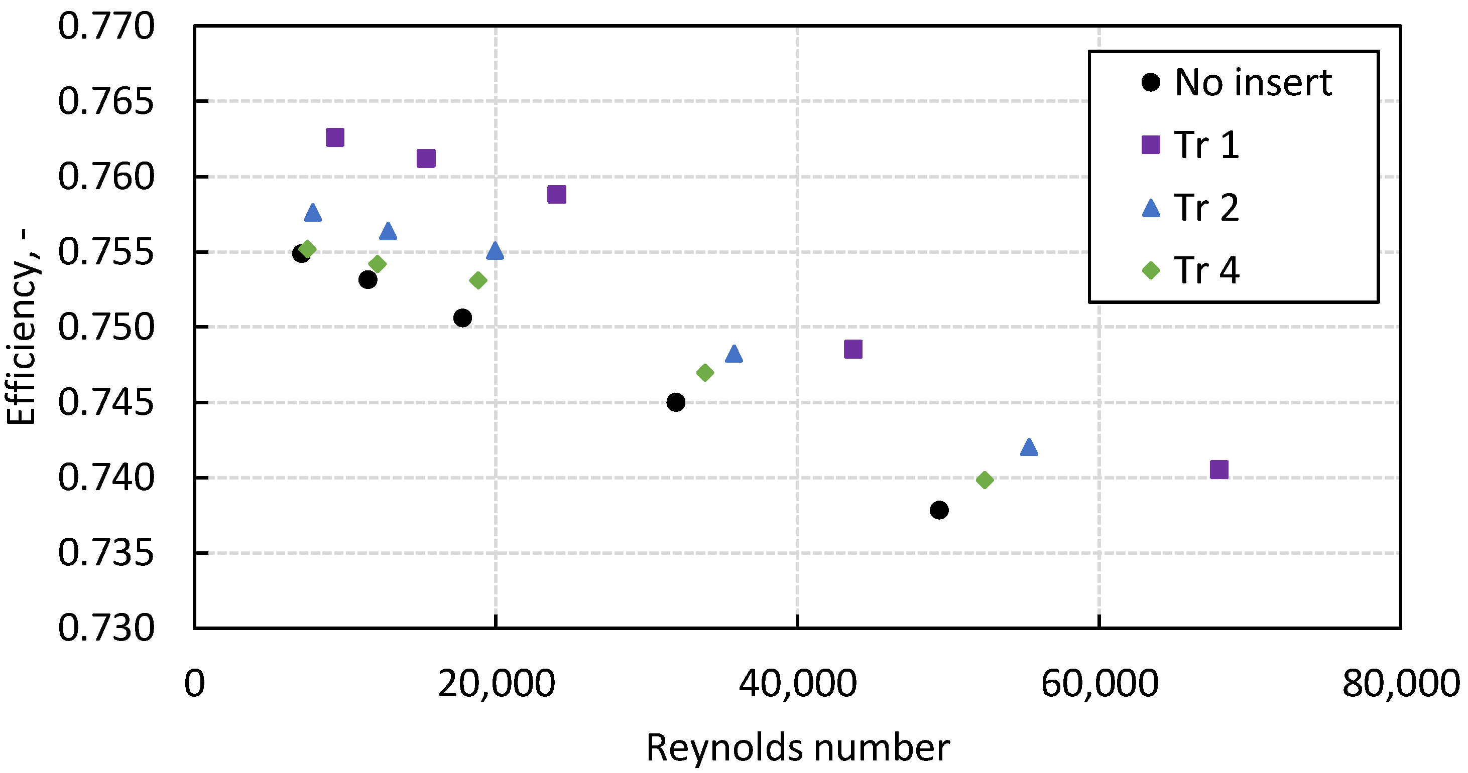
The efficiency of the parabolic trough collector (Equation (6)) as a function of Reynolds number for three analysed mass flows is presented in
Figure 18,
Figure 19 and
Figure 20. In this case, the increase in Reynolds number was due to a change in fluid temperature in analogy with the previously presented results. As the Reynolds number and fluid temperature increase, the efficiency decreases which is due to the higher wall temperature and greater heat loss to the ambient. The impact of twisted tapes is noticeable in each case. In overall terms, the absorber with insert with twisted ratio 1 has the largest increase in efficiency relative to the plane absorber. However, each of the cases analysed increases the efficiency of PTC because it reduced the wall temperature and intensifies the heat absorption. The largest efficiency gains are noticeable for low Reynolds number values. For higher flow rates and Reynolds numbers, the impact of twisted tapes is lower but still noticeable.
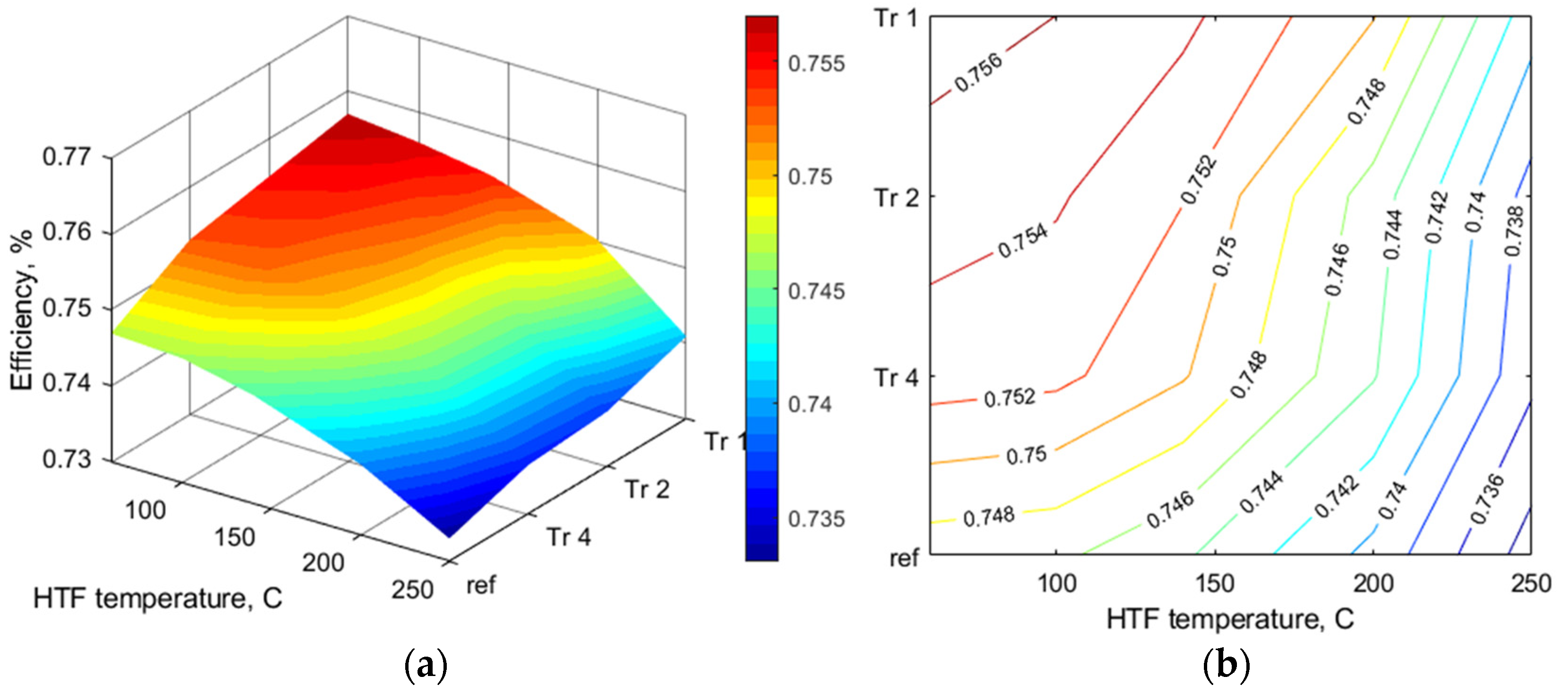
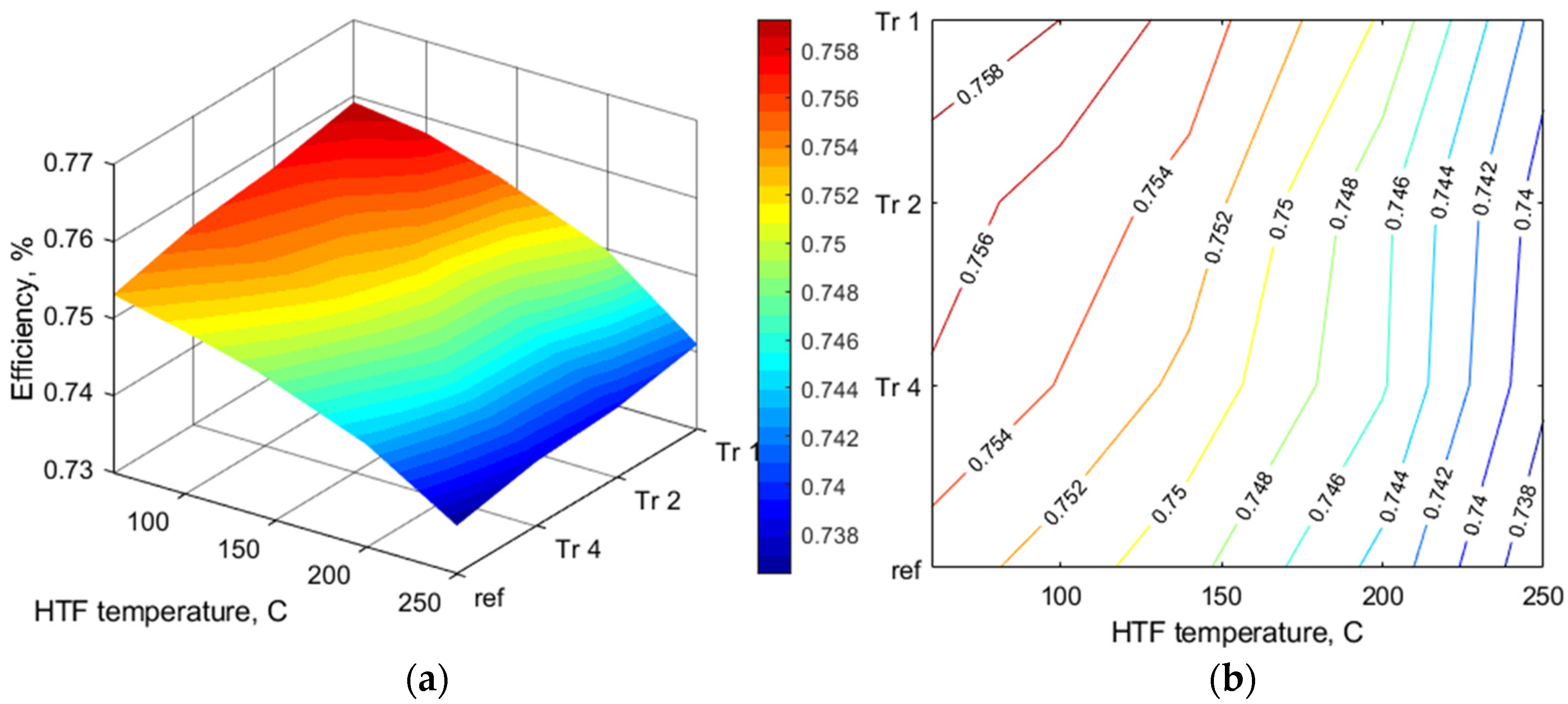
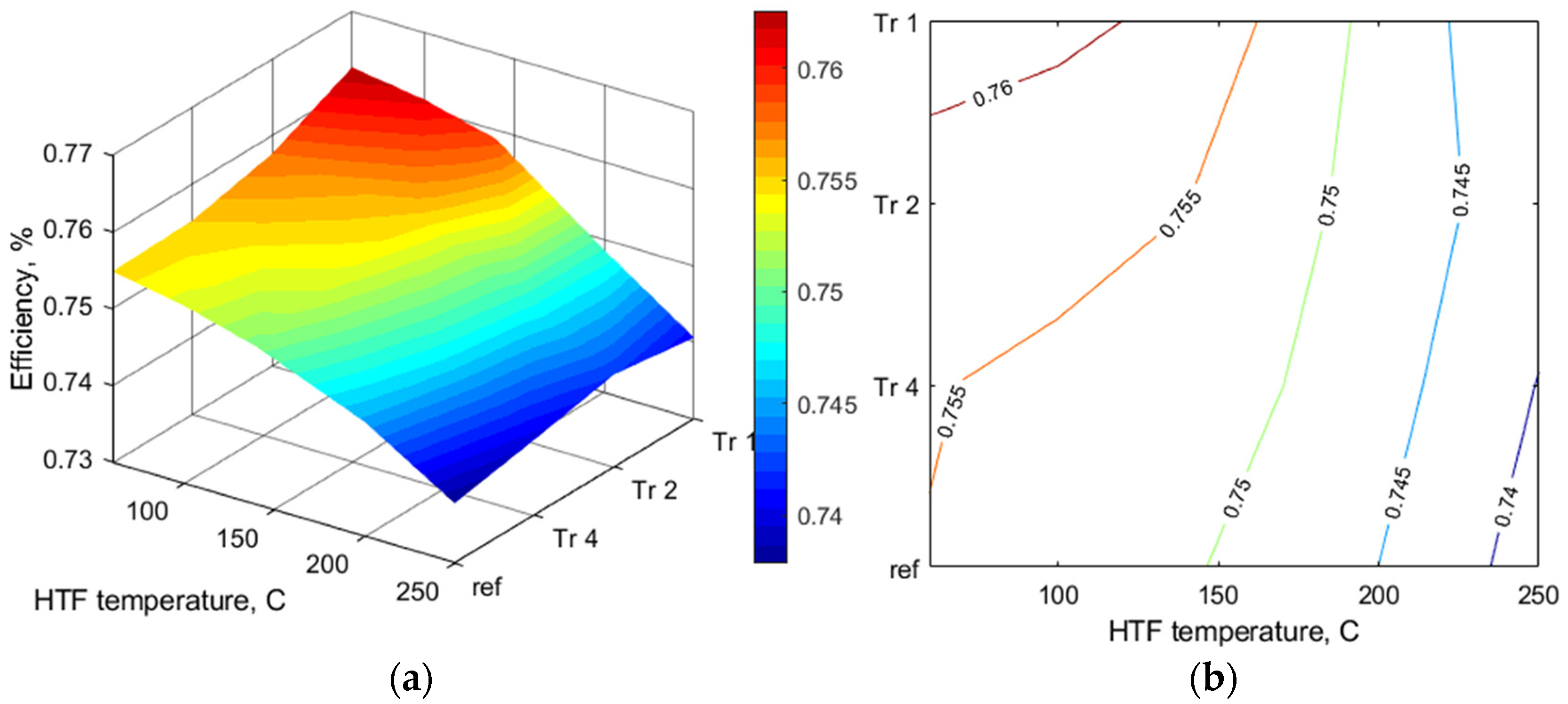
The efficiency value considers the additional friction created by the twisted tape placement inside the absorber. For the vast majority of cases analysed, the increase in pump power needed is lower than the benefit of increased efficiency, so for a wide range of flow parameters the most optimal is to use the densest insert with twisted ratio 1. Surface plots with isolines identifying efficiency levels for the analysed flows as a function of the temperature of heat transfer fluid and twisted ratio are presented in
Figure 21,
Figure 22 and
Figure 23. This estimation may allow the determination of optimum inserts with a different twisted ratio to those analysed in the numerical analysis, but their explicit determination should be pre-empted by additional numerical analysis. By analysing the efficiency of a low-concentrated parabolic trough collector system as a function of the temperature of heat transfer fluid, it is possible to identify an area where the power needed to run the pump is higher than the possible efficiency gain compared to a less dense insert. The identified area is at the end of the analysed data, for a mass flow of 0.3 kg/s and the highest heat transfer fluid temperature. In this case, it would be more optimal to use an insert with a twisted ratio of 2. It can therefore be presumed that, for potentially higher temperatures or mass flow, an increased self-requirement ratio may negatively affect the overall installation, so it may be more reasonable to use inserts with a higher twisted ratio.
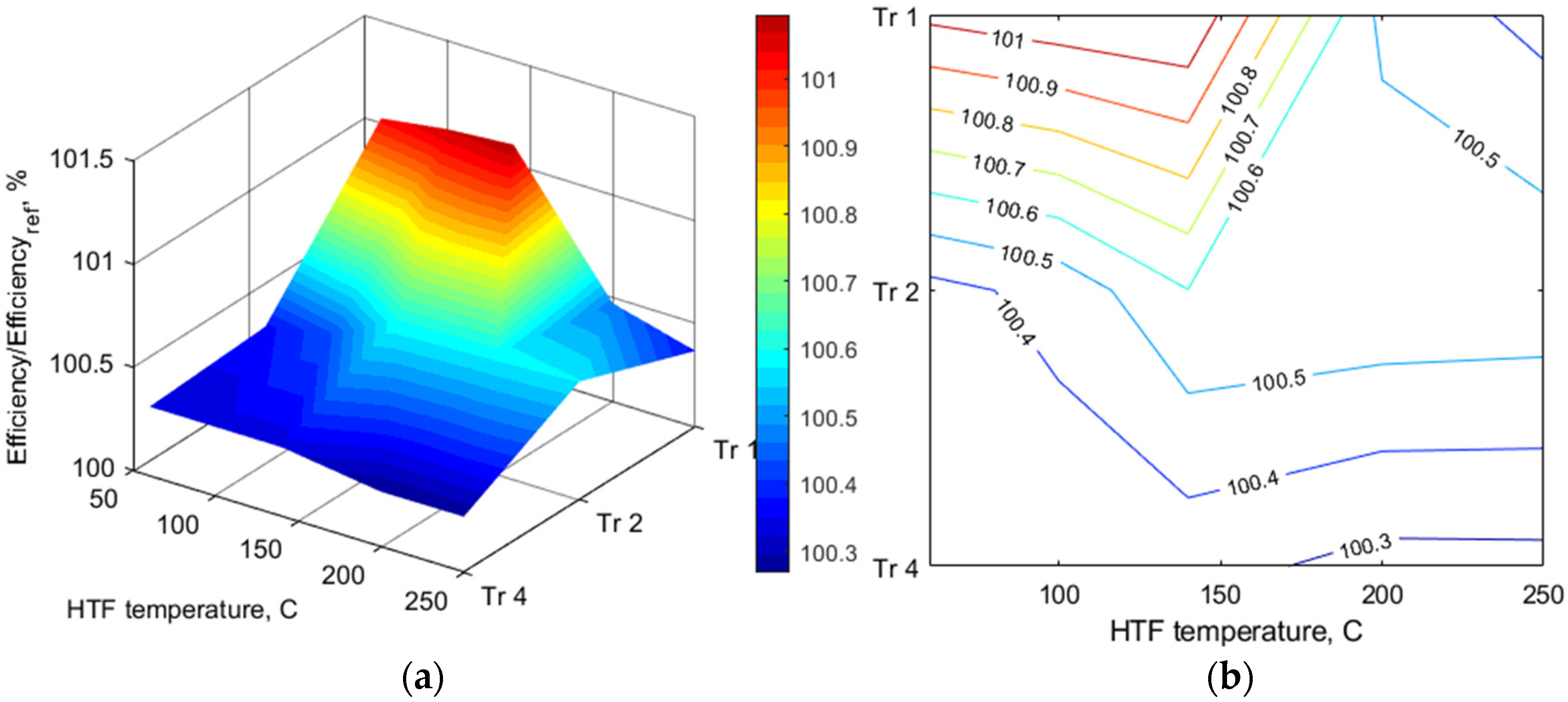
To determine more precisely the effect of an overly dense insert on installation efficiency, the PTC efficiency was compared to the reference efficiency for the same boundary conditions for a mass flow of 0.3 kg/s in which the previously mentioned area was identified.
Figure 24a,b compile this correlation as a function of temperature and the use of isolines indicates the validity of using an insert with twisted ratio 2 for temperatures greater than 190 °C.
When applying the results obtained to a solar installation, it should be pointed out that usually the mass flow in such installations is adjusted to the atmospheric conditions to achieve a certain temperature range at the outlet of the solar loop. When summarising the results for different mass flows, therefore, it is important to consider them as a comprehensive solution and to pay particular attention to the extreme results. Based on average weather data, the appropriate length of the solar loop and the conditions for adjusting the mass flow as a function of insolation can be determined. It is most desirable to operate the system for the highest designed flow rate, as this provides the highest efficiency. Therefore, for the assumed boundary conditions, flow parameters, selected fluid and geometrical dimensions, it was determined that up to a fluid temperature of 190 °C the most optimal is to use an insert with twisted ratio 1 and for higher temperatures an insert with twisted ratio 2. It should also be noted that efficiency gains relative to the reference case occur for each of the twisted tapes analysed.
3.3. Twisted Tape Application Evaluation in Long Term Analysis
To demonstrate the impact of using twisted tapes in a solar installation, a long-term analysis was carried out and the results were compared with a reference case. A previously developed mathematical model, successfully applied in the previous analysis, was used for the study [
21]. Based on the obtained Nusselt and Reynolds number increment data, relative to the reference case, a series of correlations were developed for each twisted tape and mass flow. Due to the limited range of numerical analyses, which was caused by the high computing cost and thus analysis time, it was decided that using separate correlations for each case, without estimating other mass flows, would give more reliable data. Therefore, the results of this analysis are demonstrative, presenting the potential for the use of segmental applied twisted tapes. The study analysed a case in which the installation was assumed to consist of a single solar loop, where the PTC is consistent with the geometric and optical assumptions shown in
Table 1.
The solar loop consists of 90 absorbers, each 1 m long. The inlet temperature of the solar loop, as assumed in the numerical study, is 60 °C and the outlet temperature depends on the intensity of solar radiation and mass flow. Proceeding from previous assumptions, it was determined that the facility could operate in three configurations: for mass flow 0.15 kg/s for DNI (direct normal irradiance) up to 500 W/m2, 0.225 kg/s for DNI between 500–750 W/m2 and 0.3 kg/s for DNI > 750 W/m2. This assumption results in a relatively constant temperature distribution along the length of the absorber. It should be noted that twisted tapes are mounted in a specific section of the absorber and, with variable input parameters, as is the case with renewable energy installations, there are different flow and heat transfer parameters in a given section.
The first iteration of the analysis was to clarify in which absorbers the inserts with twisted ratio 2 should be placed for the range from 750–1000 W/m2, for which the mass flow is 0.3 kg/s. In the most sensitive case, the fluid temperature reached 190 °C after the 59th absorber, so it was determined that for the entire analysis, an insert with twisted ratio 1 was used for the 59 absorber sections and an insert with twisted ratio 2 was used for the remaining 31. This ratio was maintained for the rest of the analysed cases.
The study was carried out for southern Spain location, near the town of Seville (latitude 37.41, longitude −5.75), because of the high annual insolation and the many existing installations there with concentrated PTCs [
12]. The results presented here can be used as a representation of the possible development path of these installations. Data on DNI, temperature and wind, as well as the position of the sun, were acquired using NSRDB: National Solar Radiation Database from NREL, with a resolution of 1 h [
70]. Selected climate conditions are presented in
Table 4. The study was conducted for one year, 2019.
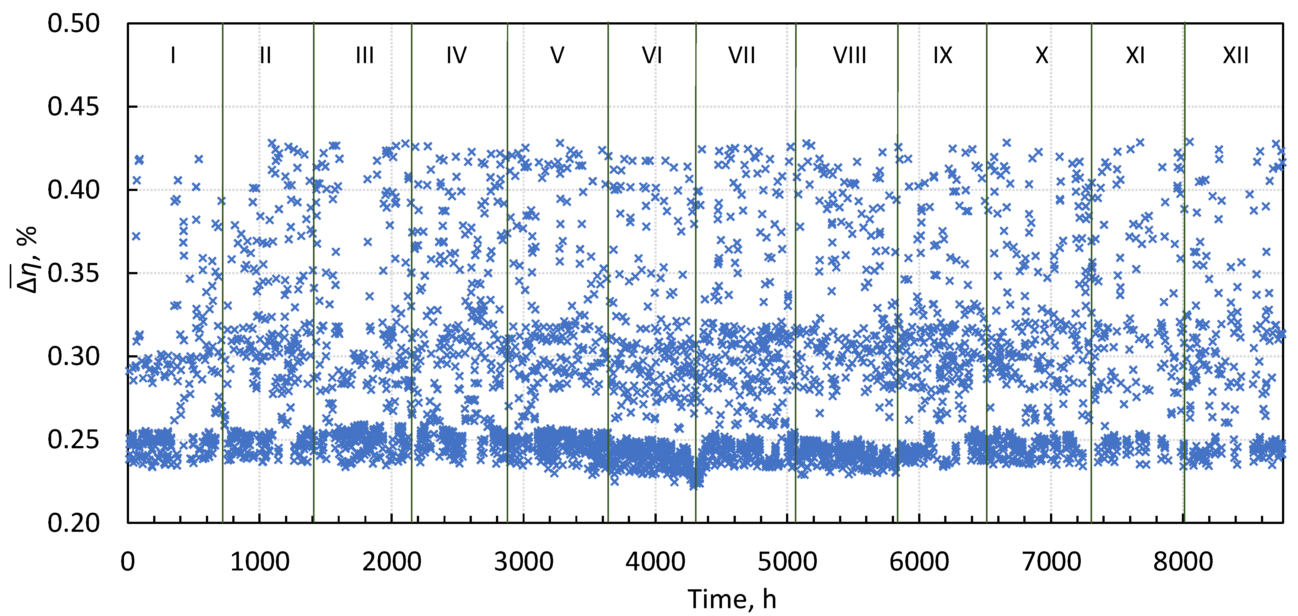
Figure 25 shows the incremental heat gain of the solar installation presented by the
factor, shown according to Equation (20):
where
Qu is the heat gained in the installation for the case with segmental arrangement of twisted tapes and without inserts, respectively.
The graph is divided into 12 parts, reflecting the 12 months of the analysed year. In each of the analysed operating hours, as long as the plant is running, an increase in the efficiency of heat extraction is visible.
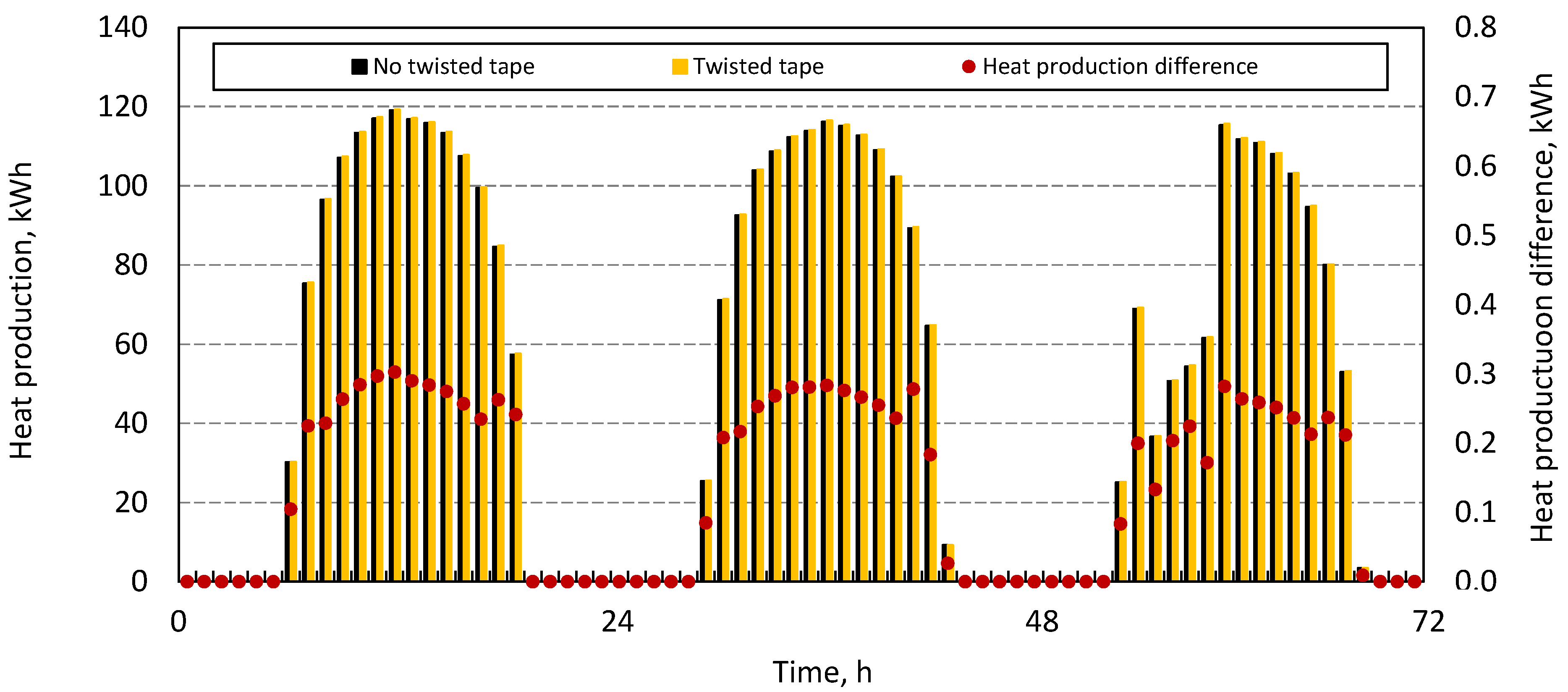
Figure 26 shows a comparison of heat production for three example days in June 2019 (1st, 2nd and 3rd). In this case, the power gain for the installation with twisted tapes is also visible. The increment in heat take-up is a maximum of 0.3 kWh for the individual hours of operation.
Comparing the results in a long-term perspective, as shown in
Table 5, the average increase in the heat generation was 0.27%. The highest average increase in one month was 0.29 in November and the lowest was 0.26 in January. The amount of heat generated by the solar installation increased by a total of 797.49 kWh. The highest production of heat occurred in June 36,093.89 kWh with no twisted tape and 36,188.97 with twisted tapes applied.


