An Optimal Scheduling Method for an Integrated Energy System Based on an Improved k-Means Clustering Algorithm

Abstract

This study proposes an optimal scheduling method for complex integrated energy systems. The proposed method employs a heuristic algorithm to maximize its energy, economy, and environment indices and optimize the system operation plan. It uses the k-means combined with box plots (Imk-means) to improve the convergence speed of the heuristic algorithm by forming its initial conditions. Thus, the optimization scheduling speed is enhanced. First of all, considering the system source and load factors, the Imk-means is presented to find the typical and extreme days in a historical optimization dataset. The output results for these typical and extreme days can represent common and abnormal optimization results, respectively. Thus, based on the representative historical data, a traditional heuristic algorithm with an initial solution set, such as the genetic algorithm, can be accelerated greatly. Secondly, the initial populations of the genetic algorithm are dispersed at the historical outputs of the typical and extreme days, and many random populations are supplemented simultaneously. Finally, the improved genetic algorithm performs the solution process faster to find optimal results and can possibly prevent the results from falling into local optima. A case study was conducted to verify the effectiveness of the proposed method. The results show that the proposed method can decrease the running time by up to 89.29% at the most, and 72.68% on average, compared with the traditional genetic algorithm. Meanwhile, the proposed method has a slightly increased optimization index, indicating no loss of optimization accuracy during acceleration. It can also indicate that the proposed method does not fall into local optima, as it has fewer iterations.

1. Introduction

In recent years, with the rapid development of industry, the world is facing increasingly serious energy shortages and environmental pollution problems [1]. To alleviate these serious problems, the use of integrated energy systems (IESs) that can combine the advantages of safety, stability, high efficiency, and low carbon emissions has become an inevitable trend [2,3]. IESs can integrate multiple energy types and energy equipment to promote the coordinated supply of different energy sources [4]. In addition, IESs can also achieve cascade energy utilization, thereby improving the efficiency of renewable energy and reducing environmental pollution [5].

Advanced energy management technology is a fundamental prerequisite for the efficient and stable operation of IESs [6], and it has become the focus of current academic research [7]. Many scholars use heuristic algorithms, such as the genetic algorithm (GA) or particle swarm optimization, to solve the optimal operation problems. Zhang et al. [8] presented a two-stage operation optimization method of IESs by using GA to optimize demand curves within customer comfort requirements. Compared with the traditional method, this method reduced operating costs by 3.6%. Jiang et al. [9] used GA with an elite retention strategy to solve an IES operation optimization model to minimize operating costs. This could reduce the system cost by 7.85% without causing environmental pollution, as well as improve the energy efficiency. To optimize the energy cost of building operation, Kamal et al. [10] used a multi-objective GA to find the best operating strategy, enabling consumers to save 10–17% of their costs each year. Li et al. [11] proposed a hybrid optimization method, using GA to optimize the hourly set value of power generation equipment. The results showed that the overall performance of this method was 1.92% better in summer and 1.91% better in winter compared with the traditional GA. Liu et al. [12] developed an IES dynamic optimization strategy based on GA, which can find the optimal transient coefficient of performance. However, this method is relatively complex, and takes 4980 s in the preprocessing stage. Zhao et al. [13] proposed a power system scheduling strategy based on a heuristic algorithm, and it can significantly reduce carbon dioxide emissions, primary energy consumption, and operating costs. This method needs to perform approximately 2,304,000 cooling and power generation simulations for 24 h, and there are cases that need more simulations and time. These optimal scheduling strategies can basically realize the stable and efficient operation of IESs. However, almost any heuristic algorithm uses a randomly generated initial solution set and requires constant iterative calculation until convergence. The optimal scheduling of IESs is characterized by complex nonlinear constraints and a large number of optimization variables. In particular, the energy storage unit also aggravates the complexity of IESs to a higher level and increases the difficulty of operation optimization [14]. These characteristics mean that the above methods take a longer time to solve optimization problems.

At present, to increase the convergence speed of optimization algorithms, many scholars use the historical data of typical or extreme periods (e.g., days or weeks) as the initial solution set of heuristic algorithms [15]. The clustering algorithm is an effective method for selecting typical and extreme periods. It divides similar profiles into clusters according to periods and then defines a representative period for each cluster [16].

To find typical periods (common values in historical data), Elsido et al. [17] used heating demand and ambient temperature to find typical periods for a heating network problem in medium-scale areas, and used them as a reference factor to evaluate annual operating costs. Li et al. [18] studied a regional IES partition optimization design method based on the clustering algorithm. This method used k-means to cluster the electricity, heating, and cooling demands, as well as the gas loads, of each building. Yeganefar et al. [19] used electricity load and electricity demand as reference factors for screening typical periods and improved the selection of the typical days of a power system. Poncelet et al. [20] first selected a small number of required representative periods and then used clustering methods to calculate and derive typical periods based on electrical load, photovoltaic power, and wind power, thus reducing the computational cost of selecting typical periods. Its accuracy is not high, because the number of original datasets in this method is small and artificially selected. The typical period selection methods used in most studies only use 2–3 influencing factors. For IESs, optimal scheduling is not only affected by the demands of cooling, heating, and power on the user side, but also has a lot to do with new energy power generation. If more clustering reference conditions and appropriate clustering methods are used, the speed and accuracy of optimization can be improved [21].

Some researchers chose the cycles with special data (e.g., peak values) as the extreme periods (abnormal values in historical data) [22]. This method only considers the peak values of a certain factor as extreme periods, and is more effective for single-factor clustering algorithms. However, it is not suitable for multi-factor clustering. Thus, the influence of other clustering factors on the results is ignored. For the multi-factor clustering algorithm, some researchers have developed algorithms that could add extreme periods to input datasets in an iterative manner [23]. For cases with a large amount of data, this iterative extreme period search method may take a lot of time because the actual extreme period may be only found in the last iteration. Zatti et al. [24] proposed an optimization-based method whose purpose is to select typical and extreme periods more accurately and systematically; the influencing factors included power, cooling, and heating. Due to the relative limitations of the considered factors, the method’s accuracy may be relatively poor in special scenarios. Li et al. [25] predicted the long-term maximum power demand of substations and conducted extreme daily searches of the forecasting process. The authors used clustering to model three common factors required by utility companies: number of customers, average demand, and installed photovoltaic capacity. In the images generated using this processing method, the points at which uneven areas appear were defined as extreme days. Sigauke et al. [26] analyzed the frequency of non-winter extreme electricity consumption peaks in South Africa. To improve the screening speed, the authors only clustered the excess parts that exceeded the power threshold on the basis of considering the demands of cooling, heating, and electricity. Although the optimization speed was significantly improved, the optimization accuracy was reduced due to a relatively small amount of data. Similar to the choice of typical periods, the choice of extreme periods also has the problem of fewer reference factors. According to current studies, most researchers tended to use the empirical method to select extreme periods, so the influence of subjective factors is relatively large.

In conclusion, at this stage, there are not enough clustering reference attributes to select the typical and extreme periods of IESs. At the same time, the selection of extreme periods mostly uses the peak value method or empirical method, making the results less comprehensive or subject to human influence. In addition, the calculation speed and accuracy of some optimization methods are not balanced, resulting in poor overall results.

This paper attempts an increase in optimizing speed without losing accuracy for the scheduling method for complex IESs. The optimization model is established based on energy, economic, and environmental evaluation indicators. An improved GA is proposed to solve this and obtain the optimal operation plan of each device. More specifically, the historical operation data of an IES are clustered using the k-means combined with box plots (Imk-means) clustering method, considering both the source (photovoltaic power and wind power) and load (cooling, heating, and electricity demands) factors. Its cluster results are used as a part of the initial feasible solution set of the GA to accelerate the convergence speed of the optimization process. At the same time, some random initial feasible solutions are employed to prevent the optimization from falling into local optima. Case studies are conducted to verify the effectiveness of the proposed method.

2. System Statement

2.1. Structure of IES

The structure of an IES with thermal energy storage (TES) is shown in Figure 1 [13]. The power generation unit (PGU) is the core component of this system, and uses natural gas to generate electricity. Photovoltaic power (PV) and wind power (WP) are employed to generate electricity. The system can also purchase electricity from the power grid to ensure the balance of energy supply and demand, and the excess electricity generated by the PGU, PV, and WP can be sold to the grid. The waste heat from the PGU is directly supplied for the heat demands of users or drives an absorption chiller (AC) for cooling. The TES can store the surplus heat energy and releases it according to the heat balance. If the heat supply is insufficient, a gas boiler (GB) will be used. Similarly, if cooling is insufficient, an electric chiller (EC) can complement it.

2.2. Energy Flow Analysis

Before analyzing the energy flow, it is necessary to clarify the operating parameters of each device. The standard characteristic data of a naturally aspirated small unit are used as an example [27]. The electricity balance of the IES can be expressed as follows:

$$E\left(t\right)=E_{pgu}\left(t\right)+E_{pv}\left(t\right)+E_{wp}\left(t\right)+E_{grid}\left(t\right)-E_{ech}\left(t\right)$$

(1)

where $E\left(t\right)$ is the electricity load in the period $t$; $E_{pv}\left(t\right)$, $E_{wp}\left(t\right)$, and $E_{pgu}\left(t\right)$ denote the output power values of PV, WP, and PGU, respectively; $E_{grid}\left(t\right)$ is the purchased ($E_{grid}\left(t\right)>0$) or sold ($E_{grid}\left(t\right)<0$) electrical energy from or to the grid; and $E_{ech}\left(t\right)$ is the input power of the EC.

Due to the fluctuations in renewable energy generation, the PGU generally operates in the off-design performance mode. Hence, the natural gas consumption of the PGU is calculated as follows:

$$G_{pgu}\left(t\right)=\frac{E_{pgu}\left(t\right)}{{\eta }_{th}\left(t\right){\eta }_e\left(t\right)}$$

(2)

where ${\eta }_{th}\left(t\right)$ and ${\eta }_e\left(t\right)$ represent the thermal and electrical efficiencies of the PGU in a period $t$, respectively. They are related to the part–load ratio of the PGU, which can be formulated as follows [11]:

$${\eta }_{th}\left(t\right)=a_0+a_1{PLR}_{pgu}\left(t\right)+a_2{PLR}_{pgu}^2\left(t\right)$$

(3)

$${\eta }_e\left(t\right)=b_0+b_1{PLR}_{pgu}\left(t\right)+b_2{PLR}_{pgu}^2\left(t\right)$$

(4)

where $a$ and $b$ represent the coefficients of the polynomials.

Then, the heating balance of the IES can be expressed as:

$$Q\left(t\right)+Q_{ach}\left(t\right)+Q_{tes}\left(t\right)=Q_{he}\left(t\right)+Q_b\left(t\right)$$

(5)

where $Q\left(t\right)$ is the heating load; $Q_{ach}\left(t\right)$ is the input power of the AC; $Q_{tes}\left(t\right)$ is the stored or released heat by the TES; $Q_{he}\left(t\right)$ is the heat recovered by the heat exchangers from the PGU; and $Q_b\left(t\right)$ is the output heat of the GB. The redundant heat generated by the system is stored in the TES. If the stored heat reaches a certain value, the TES releases heat, so $Q_{tes}\left(t\right)$ can be expressed as:

$$Q_{tes}\left(t\right)=\left\{\begin{array}{l}{Q}_{ex}\left(t\right) V_{tes}\left(t\right)<\omega \\ -\omega V_{tes}\left(t\right)\ge \omega \end{array}\right.$$

(6)

where $Q_{ex}\left(t\right)$ is the redundant thermal energy, $V_{tes}\left(t\right)$ is the TES volume at time t, and $\omega$ is the release threshold. The recovered heat $Q_{he}\left(t\right)$ by the heat exchangers from the PGU can be calculated as follows:

$$Q_{he}\left(t\right)=Q_{rh}\left(t\right){\eta }_{he}$$

(7)

where ${\eta }_{he}$ is the heat exchanger efficiency, and $Q_{rh}\left(t\right)$ is the recovered waste heat.

The cooling balance of the IES can be expressed as follows:

$$C\left(t\right)=C_{ach}\left(t\right)+C_{ech}\left(t\right)$$

(8)

where $C\left(t\right)$ is the cooling load, and $C_{ach}\left(t\right)$ and $C_{ech}\left(t\right)$ are the output of the AC and EC, respectively. $C_{ach}\left(t\right)$ is produced by converting the recovered waste heat as follows:

$$C_{ach}\left(t\right)=Q_{ach}\left(t\right){COP}_{ac}\left(t\right)$$

(9)

Similar to the PGU, the AC also runs in the off-design performance mode, so ${COP}_{ac}\left(t\right)$ is calculated as follows [11]:

$${COP}_{ac}\left(t\right)=c_0+c_1{PLR}_{pgu}\left(t\right)+c_2{PLR}_{pgu}^2\left(t\right)$$

(10)

where $c$ represents the polynomial coefficients.

3. Formulation of the Optimization Problem

The main function of optimal scheduling considered in this paper can be described as follows.

Given: Optimized objective function; scheduling constraints; target area parameters; device parameters; hourly profiles within a selected period of 24 h, including predicted energy consumption, natural resources, and energy prices; historical data of the target area, including energy consumption, natural resources, and relevant weather parameters.

Determine: Maximize the optimized objective function and obtain the hourly output plan of each device within 24 h.

3.1. Objective Function

Energy, economic, and environmental indices are usually used to evaluate the performance of IESs. These three aspects correspond to the primary energy saving ratio (PESR), cost-saving ratio (CSR), and carbon dioxide emission reduction ratio (CDERR) of IESs compared with separate production (SP) systems, respectively [28,29]. Usually, the optimal scheduling method takes each day as a cycle, so the three indices also take a day as their units.

The energy objective is defined as follows:

$$I_{PESR,day}=\frac{F_{PESR,day}^{SP}-F_{PESR,day}^{IES}}{F_{PESR,day}^{SP}}$$

(11)

where $F_{PESR,day}^{SP}$ and $F_{PESR,day}^{IES}$ denote the daily energy consumptions of the SP system and IES, respectively, and they can be calculated by:

$$F_{PESR}^{SP}={\sum }_{t=1}^{24}\frac{E_{gb}^{SP}\left(t\right)}{{\eta }_{TP}{\eta }_{GR}}$$

(12)

$$F_{PESR,day}^{IES}={\sum }_{t=1}^{24}\{\frac{E_{gb}^{IES}\left(t\right)}{{\eta }_{TP}{\eta }_{GR}v}+\frac{G_{gas}^{IES}\left(t\right)}{v}\}$$

(13)

where $E_{gb}^{IES}\left(t\right)$ and $E_{gb}^{SP}\left(t\right)$ denote the purchased electrical power of the IES and SP system, respectively; ${\eta }_{TP}$ is the power generation efficiency of the power station; ${\eta }_{GR}$ is the line transmission efficiency of the grid; $v$ is a standard coal conversion factor; and $G_{gas}^{IES}\left(t\right)$ is the fuel consumption of IES in period t. $G_{gas}^{IES}\left(t\right)$ can be expressed as:

$$G_{gas}^{IES}\left(t\right)=G_{pgu}^{IES}\left(t\right)+G_b^{IES}\left(t\right)$$

(14)

The economic objective is defined as follows:

$$I_{CSR,day}=\frac{{CS}_{SP,day}-{CS}_{IES,day}}{{CS}_{SP,day}}$$

(15)

where ${CS}_{SP,day}$ and ${CS}_{IES,day}$ are the daily operating costs of the SP system and IES, respectively. They can be calculated by:

$${CS}_{SP,day}={\sum }_{t=1}^{24}\left\{K_{gb}\left(t\right)E_{gb}^{SP}\left(t\right)+{\mu }_{gas}{G}_b^{SP}\left(t\right)\right\}$$

(16)

$${CS}_{IES,day}={\sum }_{t=1}^{24}\left\{K_{gb}\left(t\right)E_{gb}^{IES}\left(t\right)-K_{gs}\left(t\right)E_{gs}^{IES}\left(t\right)+{{\mu }_{gas}G}_{gas}^{IES}\left(t\right)\right\}$$

(17)

where $K_{gb}\left(t\right)$ and $K_{gs}\left(t\right)$ denote the prices of the purchased and sold electricity by the grid at a time t; $G_b^{SP}\left(t\right)$ is the input power of the GB in the SP system; $G_{gas}^{IES}\left(t\right)$ is the natural gas consumption of the IES; and ${\mu }_{gas}$ is the price of natural gas.

The environmental objective is defined as follows:

$$I_{CDERR,day}=\frac{V_{CDERR,day}^{SP}-V_{CDERR,day}^{IES}}{V_{CDERR,day}^{SP}}$$

(18)

where $V_{CDERR,day}^{SP}$ and $V_{CDERR,day}^{IES}$ denote the daily CO₂ emissions of the SP system and IES, respectively, and they can be calculated by:

$$V_{CDERR,day}^{SP}={\sum }_{t=1}^{24}\{u_c{E}_{gb}^{SP}(t)\}$$

(19)

$$V_{CDERE,day}^{IES}={\sum }_{t=1}^{24}\{{u_{c}E}_{gb}^{IES}(t)+{u_{b}G}_{gas}^{IES}(t)\}$$

(20)

where $u_c$ is the CO₂ emission coefficient of the coal-fired power grid, and $u_b$ is the CO₂ emission coefficient of natural gas.

Each of the above energy, economy, and environment indices can be defined as the optimization objective independently. In this study, to improve the energy, economic, and environmental performance of IESs simultaneously, the weighted objective $I$ for all three indices is defined as [29]:

$$MaxI={\alpha }_1{I}_{PESR,day}+{\alpha }_2{I}_{CSR,day}+{\alpha }_3{I}_{CDERR,day}$$

(21)

where ${\alpha }_1$, ${\alpha }_2$, and ${\alpha }_3$ denote the weights of the energy, economic, and environmental objectives, respectively. They need to meet the following conditions:

$$0\le {\alpha }_1,{\alpha }_2,{\alpha }_3\le 1$$

(22)

$${\alpha }_1+{\alpha }_2+{\alpha }_3=1$$

(23)

Without loss of generality, the coefficients can be set at ${\alpha }_1={\alpha }_2={\alpha }_3=1/3$ [18,29].

3.2. Constrains

Considering the limitations of the device input and output, the following inequalities must be satisfied:

$${\theta }_{pgu}{N}_{pgu}\le E_{pgu}\left(t\right){\le N}_{pgu}\mathrm{or}{E}_{pgu}\left(t\right)=0$$

(24)

$$0\le C_{ech}\left(t\right){\le N}_{ech}$$

(25)

$${\theta }_b{N}_b\le Q_b\left(t\right){\le N}_b\mathrm{or}{Q}_b\left(t\right)=0$$

(26)

$${\theta }_{ach}{N}_{ach}\le C_{ach}\left(t\right){\le N}_{ach}\mathrm{or}{C}_{ach}\left(t\right)=0$$

(27)

$$0\le Q_{tes}\left(t\right){\le N}_{tes}$$

(28)

$$Q_{tes}\left(t\right) \le \left|Q_{tes,max}\right|$$

(29)

where ${\theta }_{pgu}$, ${\theta }_b$, and ${\theta }_{ach}$ denote the minimum load ratios of the PGU, GB, and AC, respectively. This is to prevent the light load operation of the equipment. $Q_{tes,max}$ is the maximum input/output of the TES, and $N_{pgu}$,$N_{ech}$, $N_b$, $N_{ach}$, and $N_{tes}$ are the rated capacities of PGU, EC, GB, AC, and TES, respectively.

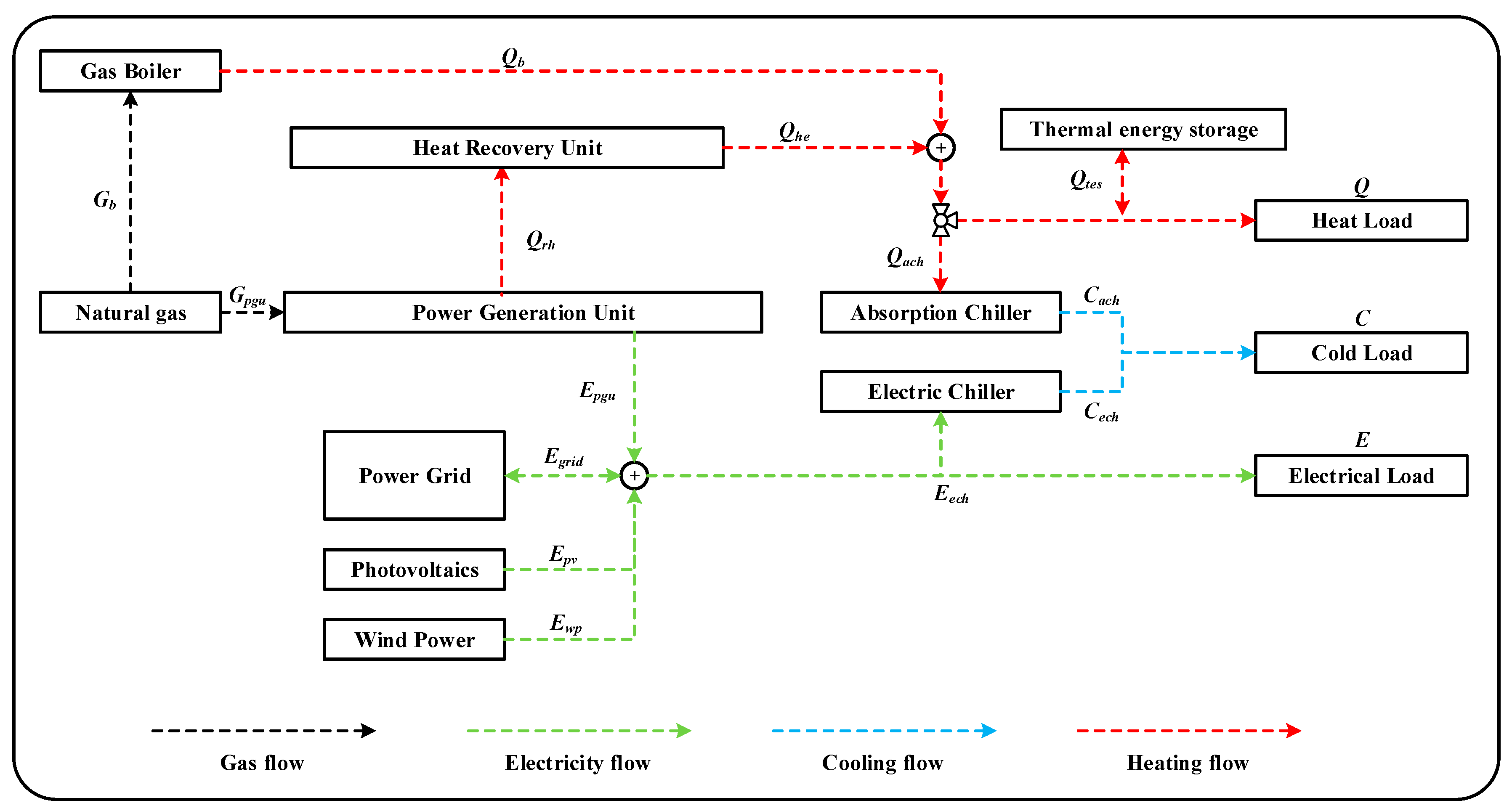
3.3. Optimization Variables

To ensure that the day-ahead optimal scheduling problem can be solved with high speed, it is extremely important to select appropriate optimization variables. The energy supply devices of the system include PGU, GB, AC, EC, and TES. If they are all regarded as optimization variables, the calculation time of the optimization algorithm will be very long. Therefore, we only selected a part of this as the optimization variables and obtained the rest of the results according to the energy flow relationship. The main energy supply equipment PGU and more controllable EC were chosen as the optimized equipment, meaning that $E_{pgu}\left(t\right)$ and $C_{ech}\left(t\right)$ are the optimization variables.

4. Optimal Scheduling Method with High Speed

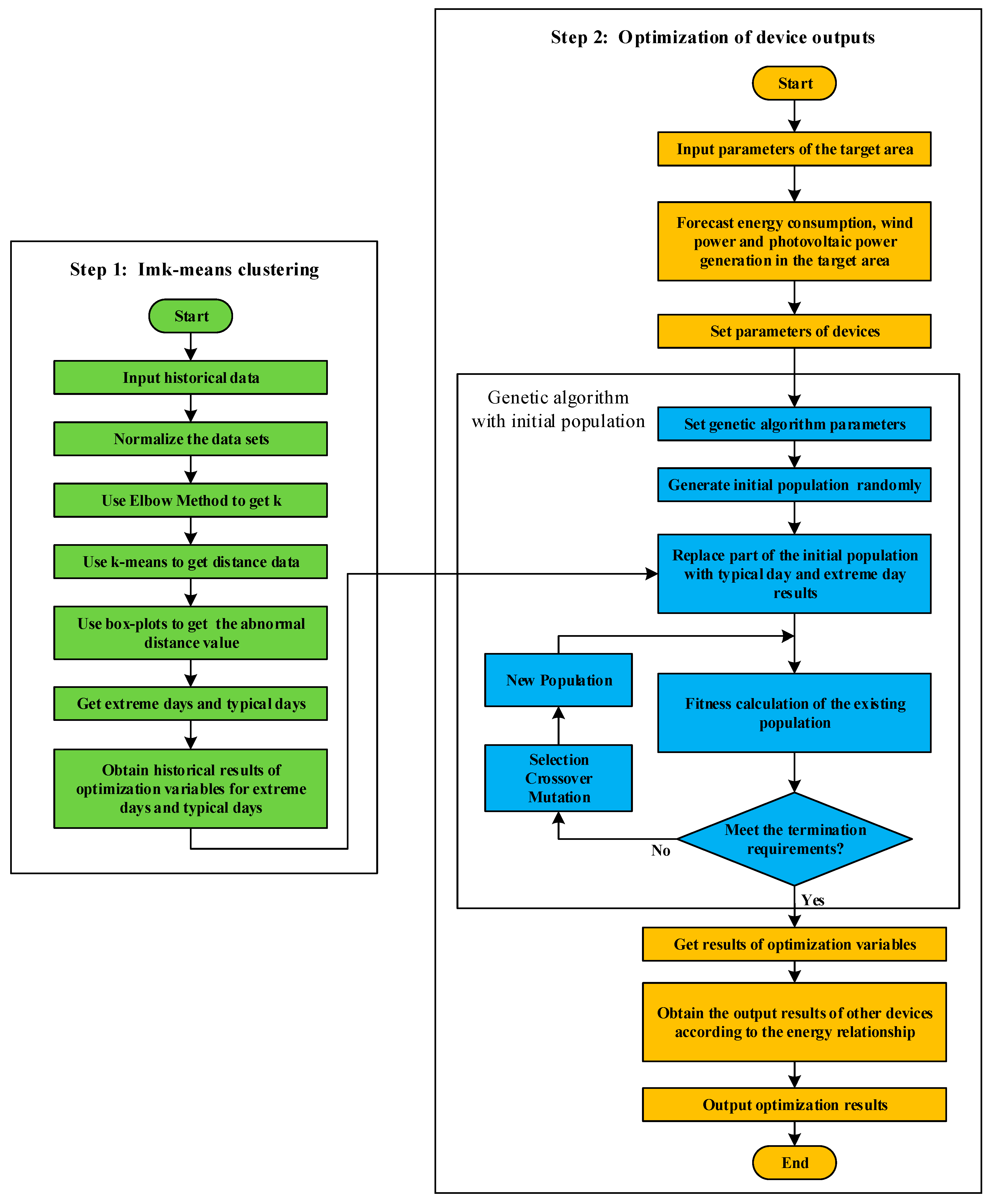
Figure 2 shows the flow chart of the proposed optimal scheduling method, which is divided into two steps. In the first step, the Imk-means is used to determine the typical and extreme periods of the historical data. Then, in the second step, the GA is employed to solve the above optimization problem, in which a part of the initial population is specified using the results of the first step. It should be noted that the historical optimization results of the typical and extreme periods determined in the first step are used to replace a small part of the randomly generated initial population. This part of the initial population can ensure the rapid convergence of the algorithm, while the remaining random population can also prevent the optimization from falling into a local optimum [30,31]. Thus, the convergence of the optimal scheduling algorithm can be accelerated without loss of accuracy. The optimization process of the second step is closed to a typical GA. The fitness of the GA is calculated using Equation (21). Therefore, the proposed Imk-means method is explained detailly in this section.

The optimal scheduling algorithm is to arrange the operation set point of each device in the next stage within a certain time step. Therefore, when accelerating the optimal scheduling algorithm, a reasonable selection of typical and extreme periods is very important. Before the next period, the operation plan of each device is obtained. In this study, we take day-ahead optimization as an example, meaning that the optimal scheduling is based on daily cycles with hourly intervals. To match the day-ahead optimal scheduling, the typical and extreme periods should also be 24 h periods. In other words, typical days and extreme days need to be found. Notably, this research method is a general method that can be used in optimization at any time interval, such as rolling optimization (optimize every 5 min), and is not limited to day-ahead optimization. If the interval time is different, only the time step $h$ in the formula needs to be adjusted. The optimal scheduling of the IESs is affected by the cooling, heating, and electricity demands, and the electricity produced by renewable energy. Therefore, the factors affecting the selection of typical days and extreme days are load (cooling, heating, and electricity demands) and source (photovoltaic power generation and WP generation). These factors are our clustering attributes.

4.1. k-Means Algorithm: Traditional Clustering Method

The k-means algorithm divides all candidates into a given number of categories by minimizing the distance between the cluster center and the other candidates [32]. This clustering method has been widely used in the optimization of IESs, especially in the case of large datasets [19]. The clustering object studied in this paper is the annual energy consumption and resource data of a certain area, so the k-means algorithm is suitable for this purpose. To eliminate the influence of different units of different clustering attributes, all data need to be standardized, as shown in Equation (30). Then, the Euclidean distance is used to calculate the distance $d(k,j)$ between the candidates, as shown in Equation (31):

$$x_{a,h,i}=\frac{{\tilde{x}}_{a,h,i}-\mathrm{m}\mathrm{i}\mathrm{n}{\tilde{x}}_{a,h,i}}{\mathrm{m}\mathrm{a}\mathrm{x}{\tilde{x}}_{a,h,i}-\mathrm{m}\mathrm{i}\mathrm{n}{\tilde{x}}_{a,h,i}}$$

(30)

$$d(k,j)=\sqrt{{\sum }_{h=1}^{24}{\sum }_{a=1}^{N_a}{(x_{a,h,k}-x_{a,h,j})}^2}$$

(31)

where $x$ is the normalized value, $\tilde{x}$ is the original value; $x_{a,h,k}$ represents the k-th clustering centroid point, and $x_{a,h,j}$ represents each attribute point; subscript $h$ is one hour within 24 h; $a$ is a clustering attribute (here, $N_a$ = 5).

Then, the k-means algorithm can be described as follows:

$$\mathrm{m}\mathrm{i}\mathrm{n}{\sum }_{j=1}^{N_j}{\sum }_{k=1}^K\{d\left(k,j\right)·z\left(k,j\right)\}$$

(32)

where $K$ is the number of clusters; $N_j$ is the number of candidates; $z\left(k,j\right)$ is a binary variable that is equal to 1 if the candidate $x_{a,h,j}$ is assigned to the k-th cluster (0 otherwise). To make sure that each candidate is exactly assigned to a cluster, constraint (33) is added.

$$z\left(k,j\right)=1\forall j\in \{1,\dots ,N_j\}$$

(33)

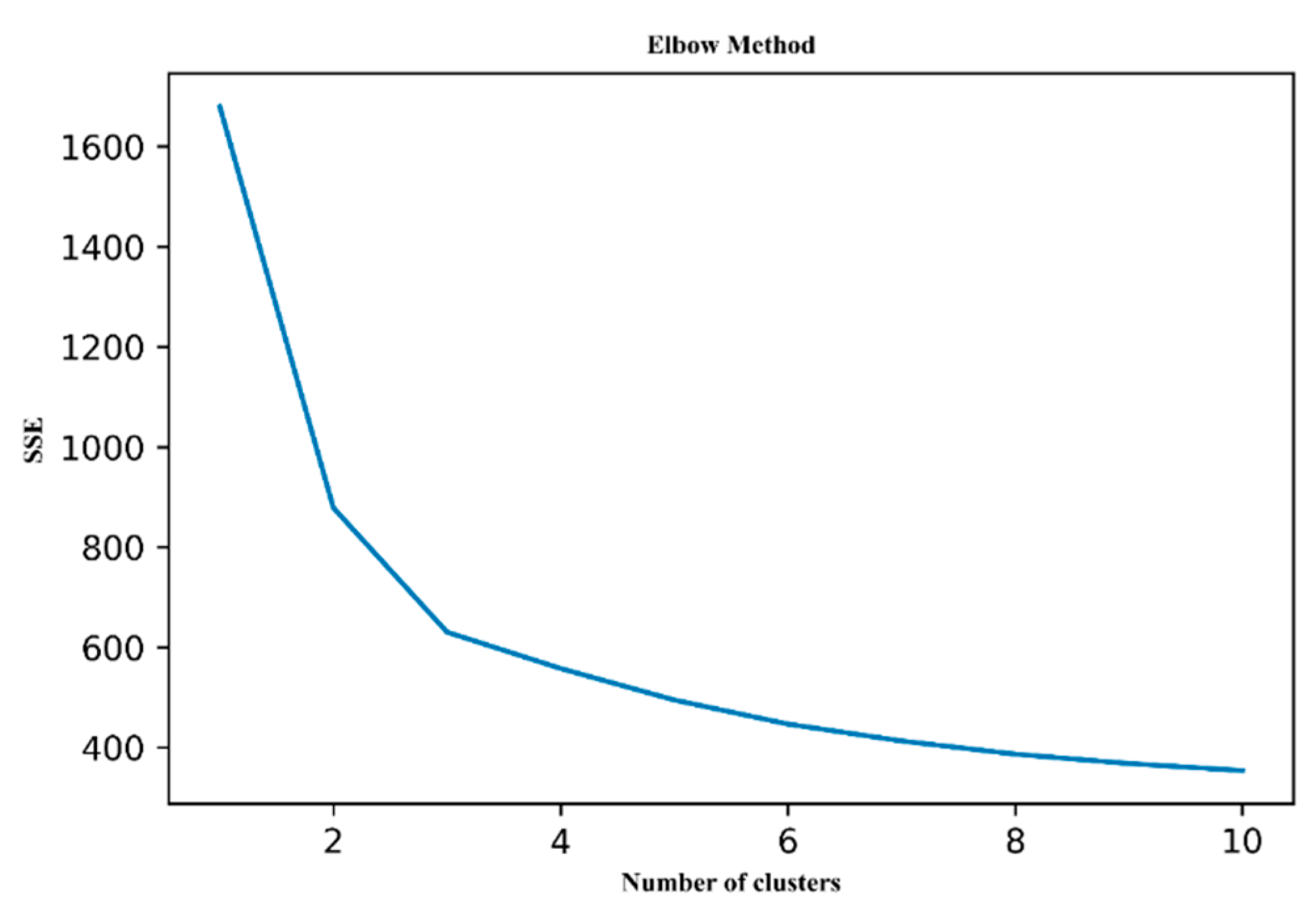
In the k-means algorithm, different values of $K$ result in different clustering results. Therefore, a reasonable choice of $K$ is very important. The elbow method is a reliable way to choose $K$. It trains multiple k-means models and makes calculations within the cluster sum of squared errors (SSE) by selecting different values of $K$. If the SSE has a sudden inflection point, the corresponding $K$ is the optimal number of clusters. SSE can be written as in Equation (34):

$$SSE={\sum }_{k=1}^K{\sum }_{j=1}^{N_j}{(x_{a,h,j}-{\stackrel{-}{x}}_k)}^2$$

(34)

where ${\stackrel{-}{x}}_k$ is the average of candidates in the k-th cluster.

In this work, the days reaching the peak value of each attribute are set as extreme days, while the other days corresponding to the clustering centroid points are set as typical days. In this algorithm, the selection of extreme days only considers a certain clustering attribute without a comprehensive consideration of all clustering attributes. This means that the k-means algorithm cannot automatically select typical days and extreme days at the same time.

4.2. Imk-Means Algorithm: A Clustering Method for Automatically Identifying Typical and Extreme Days

We developed the Imk-means algorithm that can automatically find typical and extreme days at the same time. It is essentially an improvement and adjustment of the traditional k-means algorithm combined using box plots. First, to ensure that the method can automatically select outliers (extreme days) from all candidates, constraint (33) should be changed as follows:

$$z\left(k,j\right)\le 1\forall j\in \left\{1,\dots ,N_j\right\},$$

(35)

where $z\left(k,j\right)$ is a binary variable that is equal to 1 if the candidate $x_{a,h,j}$ is assigned to the k-th cluster (0 otherwise). The constraint in Equation (35) means that each candidate does not have to be assigned to a certain cluster, where the extreme days are the candidates corresponding to $z\left(k,j\right)$ (equal to 0). Second, the extreme days need to be determined. The k-means algorithm is used to obtain the distance data for all candidates. The number of distance data is

$$N_{dis}=N_j-\hat{K}$$

(36)

where $\hat{K}$ is the number of clusters produced by the k-means algorithm. The distance data are arranged in order of size to determine the positions of $Q_1$ and $Q_3$ as follows:

$$P_{Q_1}=\frac{N_{dis}+1}{4}$$

(37)

$$P_{Q_3}=\frac{3(N_{dis}+1)}{4}$$

(38)

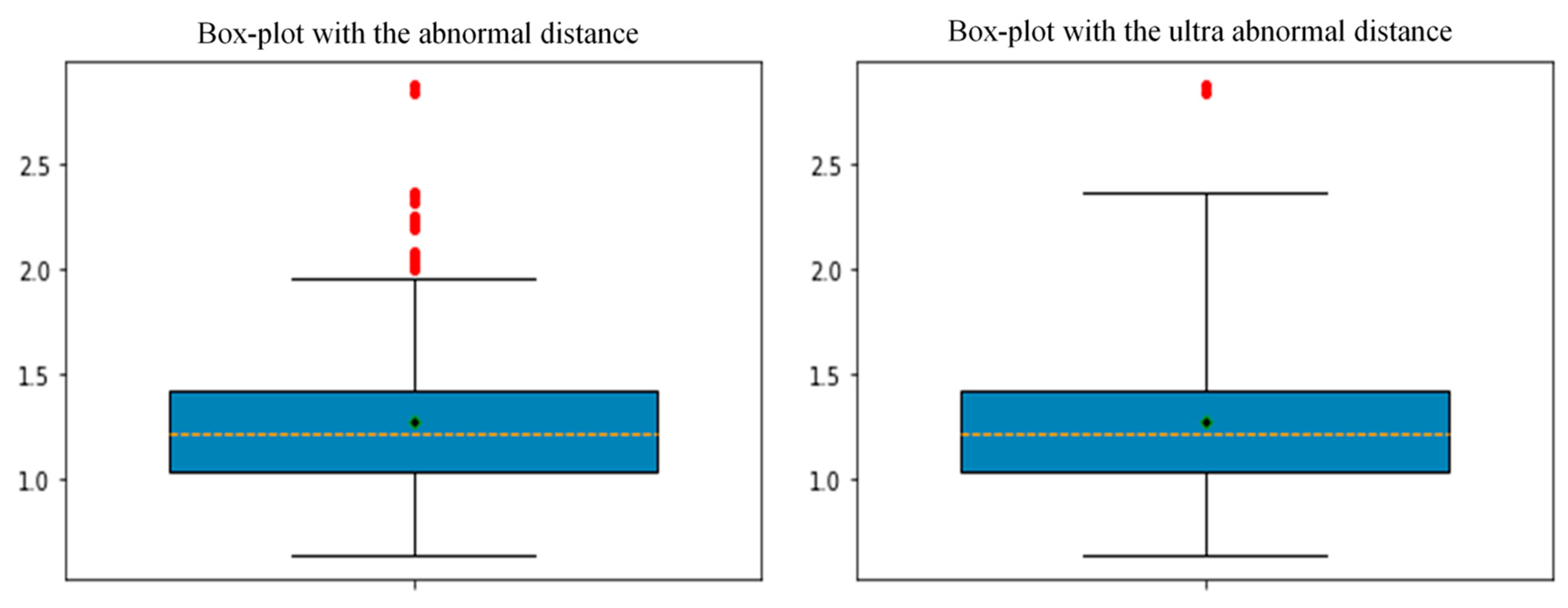
where $Q_1$ is the 1st quartile corresponding to the position $P_{Q_1}$, and $Q_3$ is the 3rd quartile corresponding to the position $P_{Q_3}$. In statistics, based on Tukey’s test, the abnormal distance value of a dataset is defined as:

$$d>Q_3+1.5\left(Q_3-Q_1\right)\cup d<Q_1-1.5(Q_3-Q_1)$$

(39)

The candidates corresponding to the abnormal distance values are the extreme days. In addition, Equation (40) defines the ultra-abnormal distance values of a dataset as follows:

$$d_u>Q_3+3\left(Q_3-Q_1\right)\cup d_u<Q_1-3\left(Q_3-Q_1\right).$$

(40)

The candidates corresponding to the ultra-abnormal distance values are the ultra-extreme days. To exclude the extreme days from the cluster candidates, constraint (41) needs to be added:

$$N_d=N_j-N_{ex}$$

(41)

where $N_d$ is the number of candidates that need to be clustered, from which the typical days are selected; $N_{ex}$ is the number of extreme days. Then, the selection of typical days can be expressed by:

$$SSE={\sum }_{\mathrm{k}=1}^K{\sum }_{j=1}^{N_d}{(x_{a,h,j}-\stackrel{-}{x_k})}^2$$

(42)

$$\min {\sum }_{j=1}^{N_d}{\sum }_{k=1}^K\left\{d\left(k,j\right)·z\left(k,j\right)\right\}$$

(43)

Equation (42) is used to determine $K$, and the clustering centroid points selected by Equation (43) are typical days.

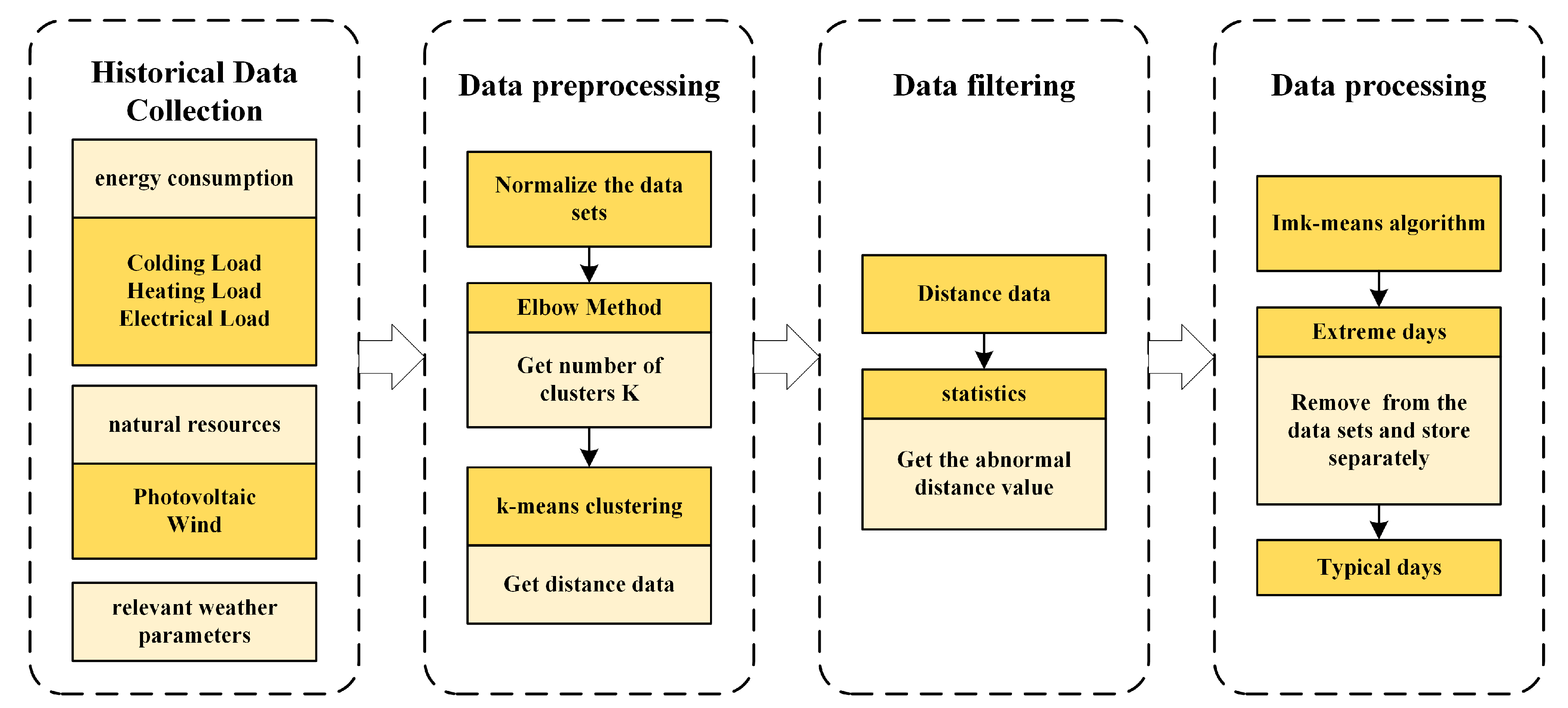
Therefore, the Imk-means method can automatically find typical days and extreme days at the same time. Unlike the traditional k-means algorithm, the calculation of $d$ includes all the clustering attributes, so the extreme days found based on $d$ also fully consider the impact of all the clustering attributes, which makes the choice of extreme days more reasonable. Figure 3 shows the process of the Imk-means method.

5. Case Study

5.1. Description of the Datasets

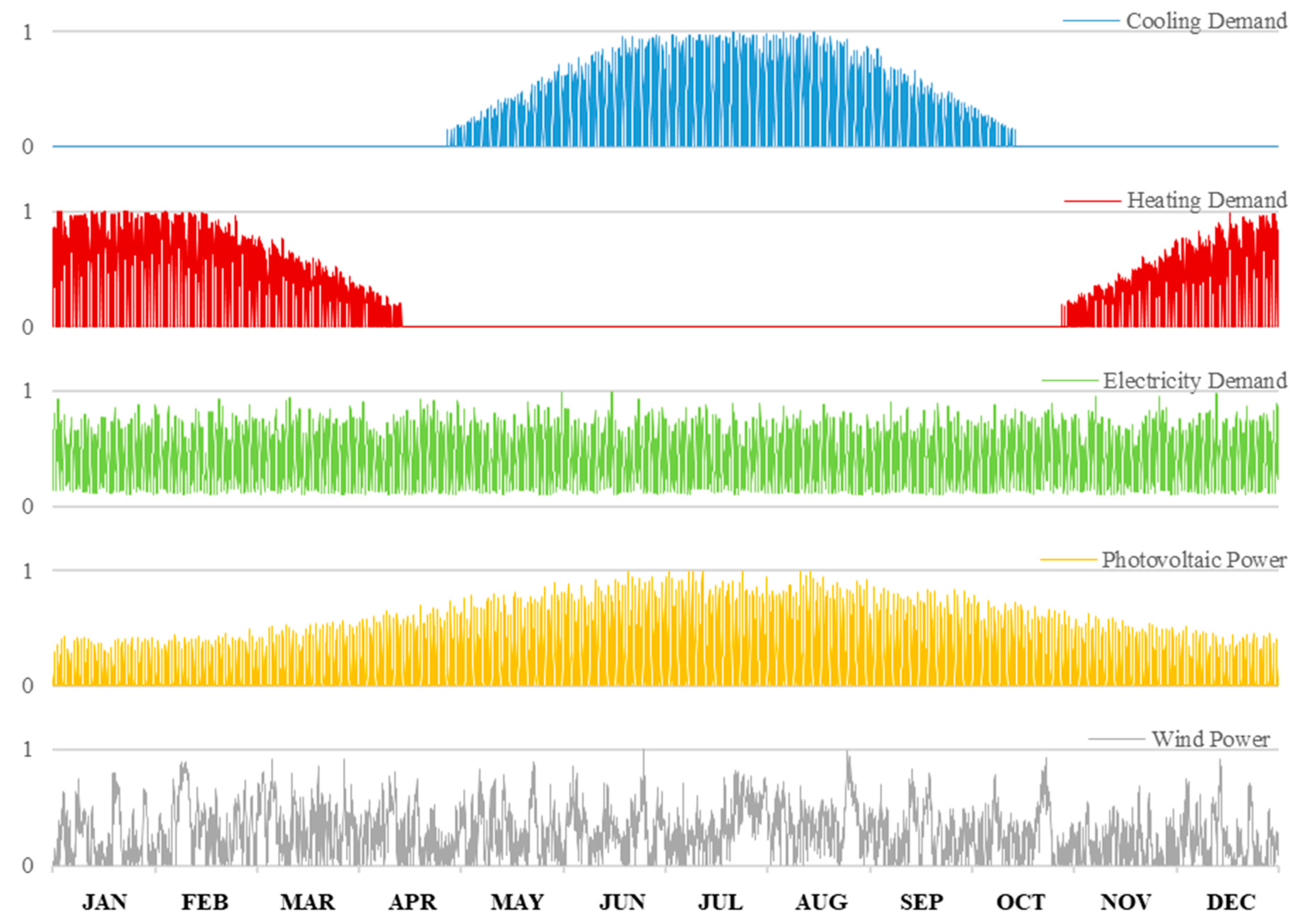
A hypothetical building in Jinan City was used to verify the proposed optimal scheduling method with high speed. The one-year time series of the relevant attributes (normalized between 0 and 1) is shown in Figure 4. The data collection interval was 1 h. These data were simulated using EnergyPlus (a software for building energy usage simulations) [33]. The following three major remarks can be made on these time series. The total electricity demand is relatively stable compared with the other attributes due to the office’s properties and the geographic characteristics of the building. Since Jinan has four distinct seasons, the seasonality of the cooling and heating demands is obvious. Photovoltaic power generation reaches its peak in summer and supplements the electricity demand for cooling. The five types of relevant attributes are divided by day, and the daily data are composed of these relevant attributes, which are combined into 120-dimensional variables as input variables for clustering.

5.2. Resource Data Clustering and Analysis

This section analyzes the processed source data. First, the number of clusters was determined by the SSE curve, and then the typical days and extreme days were determined using the proposed Imk-means algorithm. Figure 5 shows the SSE curve of the resource data. The sudden inflection point appears at n = 3, and then the curve flattens out. Therefore, when the k-means algorithm was used for clustering to obtain distance data, the initial centroid of mass was set to 3.

Box plots were used to process the distance data, as shown in Figure 6 and

Table 1. Results of the box plots.

Parameter	Value
$Q_1$	1.03696507
$Q_3$	1.42307279
$d$	2.00223437
$d_u$	2.58139595

.

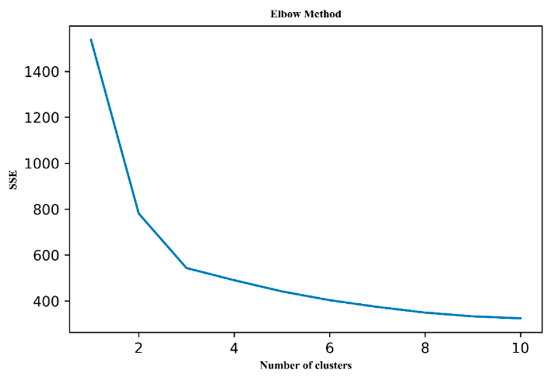
Through the data in Table 1, the distance threshold could be obtained to filter out the extreme days. After removing the extreme days from the original database, the SSE curve was recalculated, as shown in Figure 7.

As shown in Figure 7, the sudden inflection point appears at n = 3. Therefore, when the Imk-means algorithm was used for clustering to obtain typical and extreme days, the initial centroid of mass was set to 3.

Table 2. Sizes of the results.

Parameter	Size
Cluster 1	174
Cluster 2	38
Cluster 3	118
Extreme days	35

lists the size of each cluster and the extreme days.

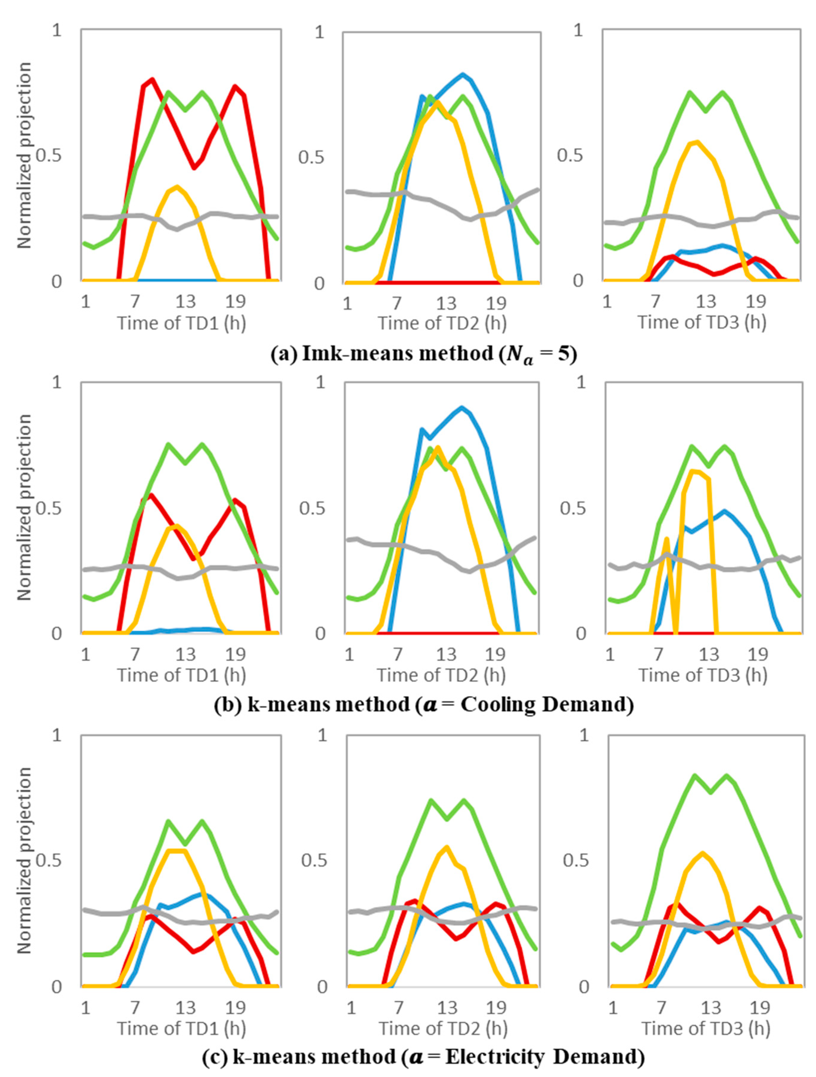
Figure 8 shows the normalized plots of the typical days selected by different approaches. The proposed Imk-means clustering algorithm in this paper is compared with the other two clustering methods, which only consider a single factor. Among them, there are three typical days: TD1–TD3. The selection of typical days used three methods from top to bottom as follows: (a) Imk-means clustering algorithm: the clustering attributes include cooling, heating, and electricity demands, as well as photovoltaic and WP; (b) K-means clustering algorithm where the clustering attribute is the cooling demand only; (c) K-means clustering algorithm where the clustering attribute is the electricity demand only.

Since both the cooling and heating demands have very obvious seasonal variation characteristics, we do not analyze the typical day selections that only considered the heating demand. It can be seen that, in a typical day obtained using the Imk-means algorithm, TD1 has a strong heat demand but no cold demand, TD2 has a strong cold demand but no heat demand, and TD3 has both cold and heat demands. This meets the three seasonal characteristics (winter, summer, and transitional seasons), which is in line with the four distinct seasons of Jinan. The typical days selected by the other two comparison methods have very sharp fluctuations, but in view of the results of a variety of factors considered together, their various attributes change relatively smoothly. From a practical point of view, under normal circumstances, none of the factors has a very obvious turning point.

Since the electricity demand of the building is relatively stable throughout the year, there are no significant differences in the electricity demand clustering results. The same phenomenon also applies to WP; because the wind does not change much throughout the year, there are no obvious differences. For the cooling and heating demands and photovoltaic power, TD3 shows a clear difference. In transitional seasons, the cooling and heating consumptions are relatively small, but they are not completely zero. This phenomenon appears to be zero when considering only the cooling demand, but it is still slightly higher in the image where only the electricity demand is considered. In the Imk-means image, the values of the cooling and heating demands are lower but not completely zero, which is more in line with reality. The proposed method in this paper can generally obtain results that are closer to reality than the methods that only consider a single factor, and the typical days derived from this method are also more accurate.

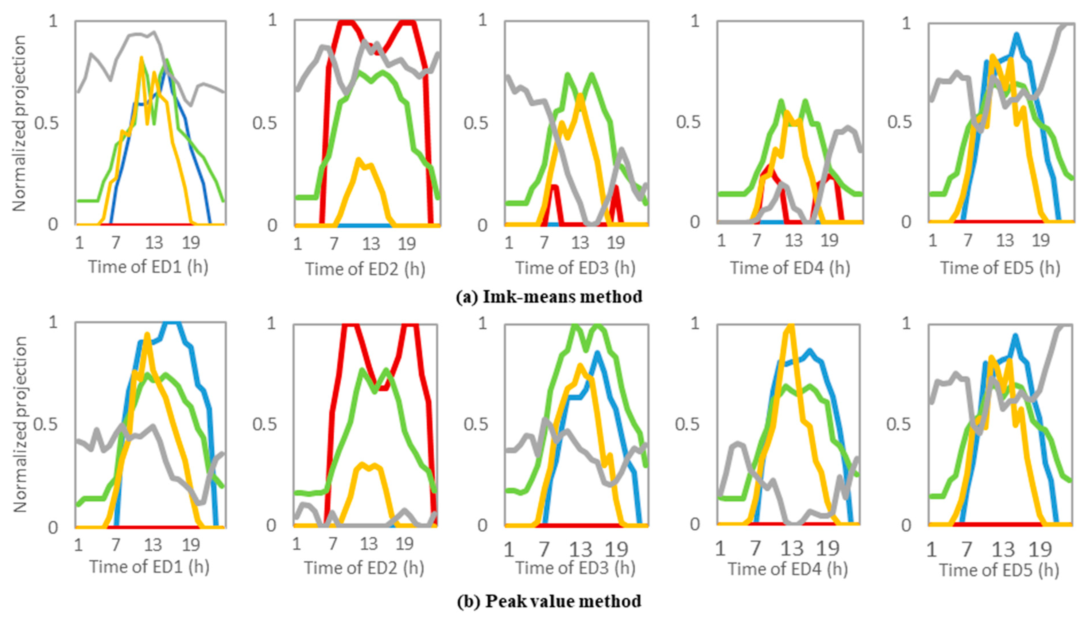
Figure 9 shows the normalized plots of the extreme days selected by different approaches. Five extreme days, ED1–5, were selected using two methods from top to bottom. The proposed Imk-means clustering algorithm clustered attributes including cooling, heating, and electricity demands, as well as photovoltaic and WP. The peak value method obtained ED1–5 when the cooling, heating, and electricity demands, as well as photovoltaic and WP, had peak values in the dataset. The extreme days obtained using the Imk-means method were slightly different from those obtained using the peak value method. The curves of selected extreme days should greatly differ from each other. If two extreme days have similar profiles, this indicates that the selection of extreme days is unreasonable. The curves of the extreme days selected by the proposed method are almost different, while some curves selected by the peak method are very similar. Compared with the extreme days selected by the peak value method, the extreme days selected considering multiple factors change more drastically, which shows that the extreme days obtained using our method are more accurate. By performing a specific analysis on a certain day, it is found that, except for ED2, the heating demands in the other four days filtered using the peak value method are all zero. However, in real life, four days with zero heat loads means that they belong to the same period (and are likely all summer days). This choice results in the cluster results being too similar to each other, and is not conducive to analysis. For the extreme days selected using the Imk-means algorithm, the types of loads that are zero in the five days are different, so they are more representative of the different conditions throughout the year. It can be seen from the ED3 and ED4 obtained using the Imk-means method that their clustering attributes fluctuate drastically and that their peak values are prominent, indicating that the days selected using this method meet the “extreme” requirements. In addition, it can be seen from ED4 using the Imk-means algorithm that, although none of the loads reach their peak during the day, each curve fluctuates sharply, satisfying the performance of extreme days. This shows that, when considering multiple factors at the same time, the extreme days are not necessarily the same days that certain data values reach peak values. The proposed method in this paper can be used to filter out such extreme days. Through comparison, the ED5s obtained by the two methods are shown to be exactly the same. The proposed method in this paper can obtain the extreme days filtered using the peak value method, and can also obtain more reasonable results under the comprehensive consideration of multiple factors. It is clear that the Imk-means clustering algorithm can automatically filter out more reasonable typical and extreme days.

5.3. Optimization Results

The GA was used as an example to analyze the speed improvement and accuracy of the designed optimization. The parameters of the equipment are shown in

Table 3. Parameters of the equipment.

Equipment	Rated Capacity (kW)	Minimum Load Ratio	Coefficient of Efficiency	Initial Energy Storage (kW)	Price (10,000 CNY/kW)
PGU	200	0.4	-	-	0.5
PV	30	-	0.85	-	1.3
WP	10	-	0.95	-	1.8
GB	700	0.3	0.82	-	0.2
AC	300	0.2	0.8	-	0.2
EC	500	-	3.5	-	0.15
TES	500	-	0.9	0	0.03

[34]. The SP system includes the EC and GB, whose capacities are obtained from the peak cooling and heating loads. The price of natural gas is 0.27 CNY/kWh [8]. The GA parameter settings are listed in

Table 4. Parameters of the GA.

Parameter	Value
Population size	200
Number of generations	100
Crossover probability	0.5
Mutation probability	0.2

.

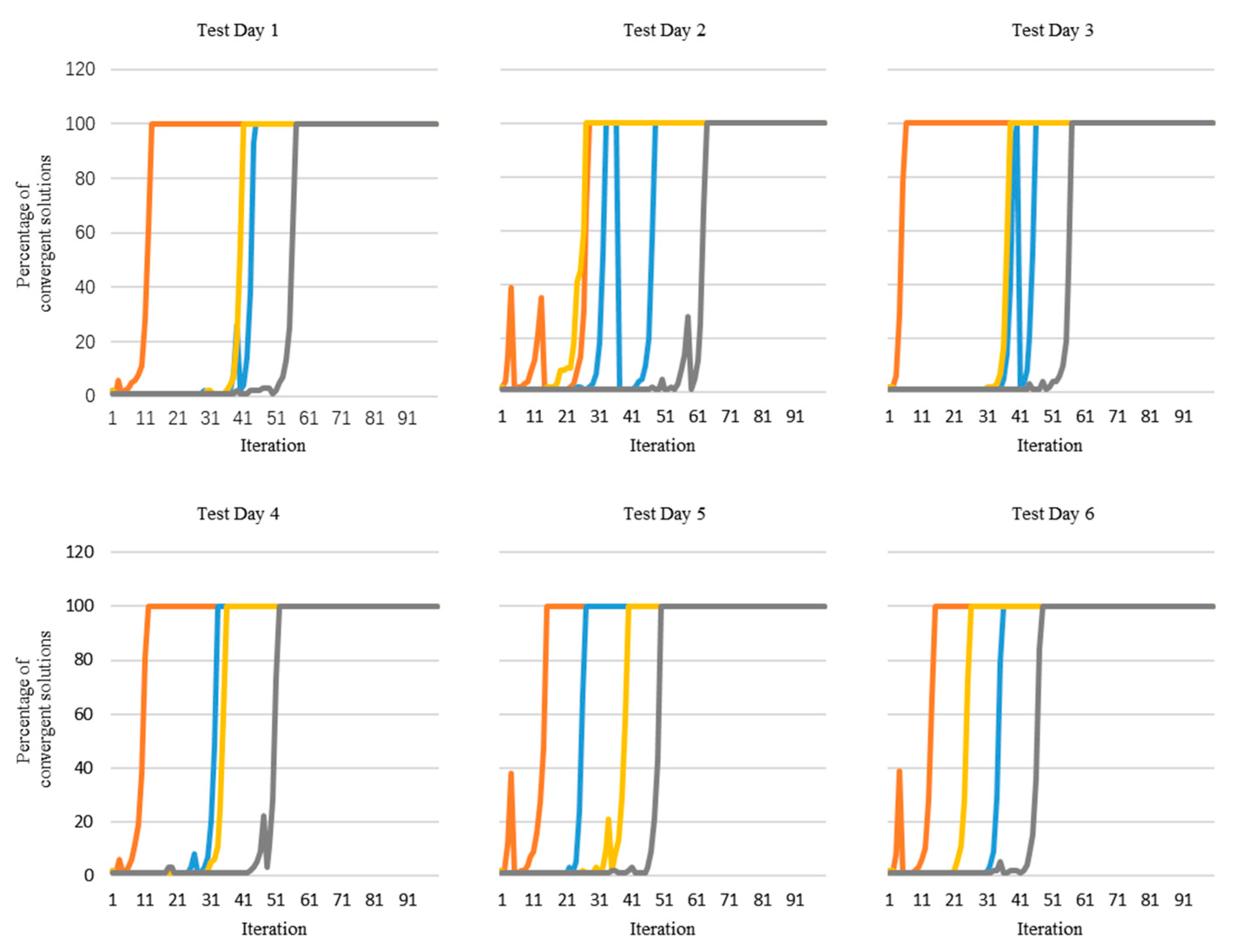
The optimization results of the typical and extreme days obtained in Section 5.2 were used as part of the initial population of the proposed optimization program, and their iterative process was compared with the improved and traditional GA, as shown in Figure 10. Six days were randomly selected as the test set, and we tried to ensure that these days included days from all the seasons during the extraction process. The details of comparison test methods are as follows: comparison test 1 used an accelerated GA, in which the typical and extreme days were selected based on the cooling demand and peak values, respectively; comparison test 2 used another accelerated GA, whose typical and extreme days were selected based on the electrical demand and peak values, respectively; comparison test 3 used the traditional GA without acceleration.

From Figure 10, it can be seen that, compared with the three comparative tests, the proposed optimization method in this study always achieved the fastest convergence. The other optimization which replaced the initial population always converged faster than the traditional GA. Therefore, it can be concluded that a suitable replacement for the initial population can indeed accelerate the convergence of optimization algorithms, and that the proposed replacement method in this paper is a more appropriate method for accelerating optimization.

To avoid contingency of the results, we ran each method 10 times to observe the average convergence rates, as listed in

Table 5. Comparison convergence results of the four methods.

Test Day No.	Methods	The Number of Iterations Required for Convergence
		1th	2nd	3rd	4th	5th	6th	7th	8th	9th	10th	Average
No.1	proposed	13	21	6	16	6	10	11	14	22	16	13.5
	test 1	45	46	45	41	36	48	54	40	59	43	45.7
	test 2	41	25	44	38	27	27	27	33	31	37	33
	test 3	57	59	45	47	62	50	50	46	53	47	51.6
No.2	proposed	28	13	13	6	6	13	15	22	12	17	14.5
	test 1	48	30	41	57	51	42	33	47	31	38	41.8
	test 2	27	24	45	48	46	22	31	17	50	38	34.8
	test 3	65	66	58	51	55	49	54	51	50	47	54.6
No.3	proposed	6	5	5	6	5	6	5	6	6	6	5.6
	test 1	46	35	35	35	51	85	71	33	27	38	45.6
	test 2	38	59	51	29	29	45	44	38	34	42	40.9
	test 3	57	58	48	49	70	48	45	50	46	52	52.3
No.4	proposed	12	6	15	6	31	14	19	36	15	6	16
	test 1	33	42	43	47	61	41	34	43	36	43	42.3
	test 2	36	39	34	57	74	86	43	15	74	32	49
	test 3	52	48	42	54	50	47	40	42	47	47	46.9
No.5	proposed	15	24	20	26	15	27	11	17	11	11	17.7
	test 1	27	55	44	37	36	31	49	49	46	51	42.5
	test 2	40	37	34	44	28	27	28	32	41	40	35.1
	test 3	50	67	39	39	57	49	49	41	49	48	48.8
No.6	proposed	15	24	22	6	5	5	27	15	13	6	13.8
	test 1	36	33	26	45	31	31	39	44	38	60	38.3
	test 2	26	24	45	30	41	33	33	49	31	39	35.1
	test 3	48	39	42	42	46	47	48	45	45	56	45.8

. The four different optimizations are the proposed method and the three other methods of comparison test 1, test 2, and test 3. From the data in Table 5, it can be seen that the conclusions are the same as those obtained from Figure 10. The proposed optimization method in this paper always converged faster.

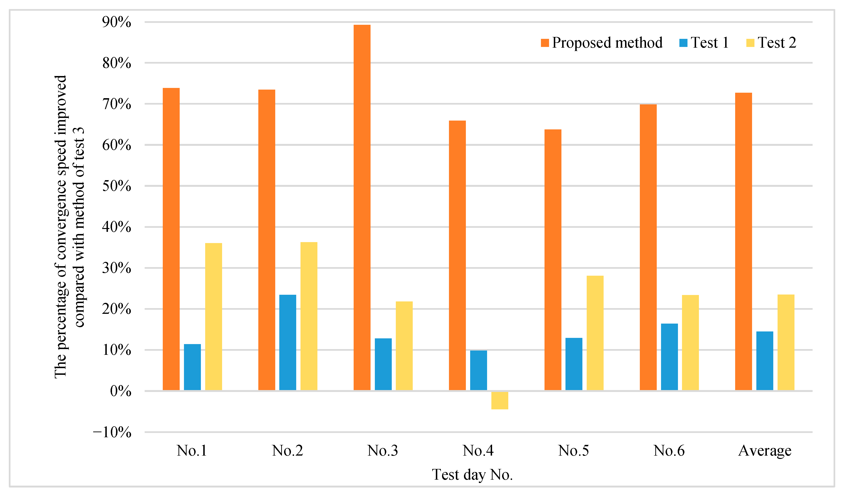
Figure 11 shows the percentage of convergence speed for the proposed method and methods of tests 1 and test 2, compared with the traditional GA used in test 3. In the randomly selected test set, the improvement in speed of the proposed method could reach up to 89.29% at best, and 72.68% on average, compared with the traditional GA. It can be seen that the proposed optimization method in this paper is, on average, 58.22% faster than the method used in test 1, and 49.17% faster than the method used in test 2. In addition, it is worth noting that the data obtained on the fourth test day in test 2 could not effectively accelerate the optimization algorithm, showing that the obtained typical and extreme days do not cover the fourth test day. This shows that the typical and extreme days obtained by the proposed method are more realistic and reliable. In summary, the proposed method can always converge faster than the other acceleration methods.

To verify that the acceleration does not lose optimization accuracy, we compared the results of the two optimizations (proposed and unaccelerated) and summarize them in

Table 6. Optimization results.

Test Day No.	PESR		CSR		CDERR
	Proposed	Unaccelerated	Proposed	Unaccelerated	Proposed	Unaccelerated
No.1	0.349068	0.307028	0.331584	0.314526	0.367105	0.367615
No.2	0.066901	0.015197	0.094727	0.063864	0.135633	0.110889
No.3	0.53121	0.464188	0.484205	0.455047	0.55152	0.54615
No.4	0.462359	0.43935	0.430054	0.415684	0.4888	0.478241
No.5	0.006422	0.020481	0.017027	0	0.025043	0
No.6	0.39973	0.370715	0.336494	0.325065	0.353632	0.355469

. The larger values of these parameters indicate better results.

To judge whether accuracy is lost more intuitively, we included parameter $∆$, which is the difference between the results of the proposed optimization and traditional GA. If $∆\ge 0$, this proves that there is no loss of accuracy. Especially, if $∆>0$, this indicates that the optimized result after acceleration is better, as shown in

Table 7. Results of parameter $∆$.

Test Day No.	$∆$PESR	$∆$CSR	$∆$CDERR	$∆$I
No.1	0.04204	0.017058	−0.00051	0.019529333
No.2	0.051704	0.030863	0.024744	0.035770333
No.3	0.067022	0.029158	0.00537	0.03385
No.4	0.023009	0.01437	0.010559	0.015979333
No.5	−0.01406	0.017027	0.025043	0.009336667
No.6	0.029015	0.011429	−0.001837	0.012869

.

By observing the parameter $∆$ for the energy, economic, and environmental indexes, and the weighted objective I, it can be seen that the weighted objective values of the proposed optimization are all better than the traditional GA. Though $∆$ parameters have negative values, −0.00051, −0.01406, and −0.001837, the other indices will counteract these negative values. Thus, the proposed optimization algorithm in this study does not reduce the optimization performance and even can improve it to a certain extent. Therefore, the case study demonstrates that the proposed optimization method can greatly increase the calculation speed without losing optimization accuracy. The optimization results of the improved algorithm are very close to those obtained by the traditional algorithm, and their hourly output plans are almost identical. Thus, the differences in their output plans will not be discussed in the case study of this paper.

6. Discussion

The proposed Imk-means clustering method in this paper considers both the source factors (photovoltaic power and WP) and load factors (cooling, heating, and electricity demands). It can obtain typical daily clustering results, which are more consistent with the actual situation of energy supply throughout the four seasons. For spring and autumn, the values of the cooling and heating demands are both lower, which is more in line with reality. It can also obtain extreme day clustering results that differ from each other. This indicates that the selection of extreme days using the proposed method is more reasonable and accurate compared with the peak value method.

For a heuristic algorithm such as the GA, some of the feasible solutions can be dispersed around the equipment output results of these clustering typical and extreme days, and a large number of random feasible solutions are also preserved. Thus, the improved heuristic algorithm can achieve faster convergence and fewer iterations, which leads to a faster computation time without affecting the optimality of the results. In the case study, the optimization results of the improved method are slightly better than those obtained with the traditional GA method.

7. Conclusions

This paper proposes an improved heuristic optimization method for the operation of IESs. It can increase the computing speed of the traditional heuristic optimization without losing optimization accuracy. For the GA, its initial populations took advantage of the equipment output results of the clustering of typical and extreme days, thereby greatly increasing its solving speed. Using the Imk-means clustering method, the source factors (photovoltaic power and WP) and load factors (cooling, heating, and electricity demands) were comprehensively considered to scientifically and accurately determine the typical and extreme days of the historical datasets. In order to prevent the results from falling into local optima, many random populations were supplemented simultaneously. The case study verified the effectiveness of the proposed method. The results are as follows.

• The typical and extreme days obtained in this study are more accurate and in line with system requirements compared with those obtained using the existing methods. They can be used to accelerate the system convergence faster than the existing methods.
• The convergence speed of the optimization algorithm increased by up to 89.29% compared with the traditional GA, and the average speed increased by 72.68%. While speeding up, the optimization performance undergoes a small performance improvement.

In addition, with the growth of historical databases, the search for typical and extreme days will be more reasonable and more suitable for systems, so a more effective optimization and acceleration will be obtained. Future work will focus on the combination of artificial intelligence and optimization methods to extract useful information from historical data, and further explore the efficiency of energy savings and emission reductions achieved by the system.