Article

Emerging Parameters Extraction Method of PV Modules Based on the Survival Strategies of Flying Foxes Optimization (FFO)

1
Laboratory of Engineering and Materials (LIMAT), Faculty of Sciences, Ben M’Sick Hassan II University of Casablanca, Casablanca 20000, Morocco
2
Laboratory of Agricultural Engineering, Energy National Institute of Agricultural Research Settat, Settat 26000, Morocco
3
Matter Physics Laboratory (LPM), Faculty of Sciences, Ben M’Sick Hassan II University of Casablanca, Casablanca 20000, Morocco
*
Author to whom correspondence should be addressed.
Energies 2023, 16(8), 3531; https://doi.org/10.3390/en16083531
Submission received: 18 February 2023 / Revised: 31 March 2023 / Accepted: 6 April 2023 / Published: 19 April 2023
(This article belongs to the Special Issue Analysis and Numerical Modeling in Solar Photovoltaic Systems)

Abstract

:
Nowadays, the world is encountering multiple challenges of energy security, economic recovery, and the effect of global warming. Investing in new fossil fuels only locks in uneconomic practices, sustains existing risks and increases the threats of climate change. In contrast, renewable energies, such as photovoltaic energy, constitute one of the most promising technologies in combating global increase in temperatures. Given its simplicity and low maintenance costs, photovoltaic energy is the most effective alternative to address the issues above. However, the standard test conditions (STCs) of PV modules are, in most cases, different from the real working conditions of a solar module. For instance, high levels of incident irradiation in an arid climate may cause the temperature of a module to rise by many degrees above the STC temperature of 25 °C, lowering the module’s performance. To effectively simulate and control PV systems for a given location, it has become paramount to develop a robust and accurate model that considers how PV modules behave. This study seeks to introduce an emerging metaheuristic optimization algorithm to estimate the unknown parameters of PV modules. The strategies deployed by flying foxes in the event of high temperatures have given birth to the development of a new metaheuristic algorithm called FFO. Contrary to previous methods, this new modeling procedure makes it possible to calculate all the parameters, regardless of temperature or irradiance. Four PV modules, having different technologies, were tested to evaluate the accuracy of the algorithm in question. The effectiveness of FFO is then contrasted with other well-known metaheuristics where single and double diode models are deployed. The results show that the FFO optimizer represents a substantial and compelling substitute for PV module extraction methods.

1. Introduction

Given the ongoing rate of energy transition, instant and radical action is necessary to significantly reduce the chance of being above the 2 °C path. The financial repercussions of natural catastrophes have become driven and intensified and far exceed the costs of such energy transformation. Furthermore, the current crisis in Ukraine raises new levels of concern and uncertainty, negatively affecting the costs to economies that remain profoundly dependent on fossil fuels. Such issues certainly speed up the depletion of non-sustainable energy sources. Sustainable energy continues to gain ground against such energy resources as fossil fuels [1]. Wind and photovoltaic energies, as primary renewable energy sources, have witnessed enormous development in recent decades. Some of the prominent advantages of photovoltaic energy include popularity and low cost. According to a report, published by the International Renewable Energy Agency (IRENA), in 2021, the cost of solar photovoltaic modules has declined over the past decade, with the global weighted average cost falling by around 90% between 2010 and 2020. The growing demand for a PV system has driven researchers to elaborate numerous methods and approaches to deeply understand the reaction of a solar module to different meteorological changes. The implementation of precise modeling of a PV system, to help designers improve solar energy efficiency, still poses a great challenge. Over the years, many methods have been adopted in the literature that use the most basic single diode model as the starting point and then move on to more sophisticated models, such as the double diode model [2,3,4,5,6,7]. Undoubtedly, the greater the complexity of a model, the higher the number of parameters included in its computation. The prevailing usage of the single diode model by the vast majority of researchers is due to the fact that it perfectly balances simplicity and accuracy. However, it disregards the recombination effect in the depletion region, which is relevant a real solar cell. For this reason, a better and more sophisticated model, referred to as the double diode model, was established [8,9,10,11,12]. Nevertheless, the complicated nature of this model could be attributed to the number of parameters involved and the non-linearity of its distinct equations. The implementation of a single diode model requires the estimation of the following five parameters: the photocurrent ( I p h ), the diode ideality factor (a), the reverse saturation current ( I 0 ), the series and the shunt resistance ( R s , R s h ). The integration of another diode results in there being seven parameters for the double diode model. The new parameters are the reverse saturation current ( I 02 ) and the ideality factor ( a 2 ) linked to the second diode. In order to calculate the unknown parameters of the mentioned models, a variety of approaches are proposed in the literature.
The analytical method is the most commonly used approach for extracting PV parameters. This method applies to the technical datasheet provided by the manufacturer. The equations draw on the most prominent points on the I–V curve, especially the current and the voltage at short circuit ( I s c ), the open voltage ( V o c ), and the maximum power point (MPP). Besides these points, other equations may also be deployed, such as the reciprocal of slopes at the short circuit and open circuit conditions and the derivative of power at the maximum power point [13,14,15].
Recently, and due to their considerable potentials, various optimization metaheuristic algorithms have been proposed in studies focusing on extracting PV module parameters, including the following: Differential Evolution (DE), Particle Swarm Optimization (PSO), Artificial Neural Networks (ANN), Invasive Weed Optimization (IWO), Cuckoo Search (CS), Genetic Algorithm (GA), Firefly Algorithm (FA), and Chaotic Whale Optimization Algorithm (CWOA). The metaheuristic algorithm, employing a global optimization search approach, offers superior performance compared to the analytical method. It delivers high solution accuracy and is well-suited for addressing multi-dimensional problems. As computer science continues to evolve, the metaheuristic algorithm has emerged as the preferred method for solving PV parameter identification problems [16]. Given their abilities in global searches, they are considered very efficient in handling complex optimization equations, regardless of the amount of information provided [17,18,19,20,21].
This paper presents a state-of-the-art metaheuristic algorithm, based on the survival strategies of flying foxes in the event of high temperature (FFO), to extract PV module parameters, using only the information provided by the manufacturer at the three remarkable points on the I–V curve. A few parameters are optimized using FFO, while the others are calculated analytically. Given that the variety of most metaheuristics depends heavily on the initial parameters [22], the suggested approach deploys a fuzzy self-tuning method to carry out accurate calculations at each iteration. Contrary to some anterior methods, the proposed algorithm computes the unknown parameters at every change in environmental conditions of temperature and irradiation. The efficiency of FFO is juxtaposed with other well-known metaheuristics algorithms adopting single and double diode models. Moreover, it is approved through data from four PV models of diverse types.
This study is divided into four further sections. The second section introduces mathematical equations describing single and double diode models. In Section 3, the adopted algorithm is summarily introduced, including the expression of the objective function. Section 4 explains the assessment of the adopted optimization approach against similar prominent techniques, and Section 5 provides a summary of the significant findings of the study.

2. Circuit Analyses of Single and Double Diode Models

This part presents the electrical equivalent circuit of the single and double diode models. Next, it provides mathematical equations that illustrate the functioning of a solar cell at open voltage, short circuit current, and maximum power point.

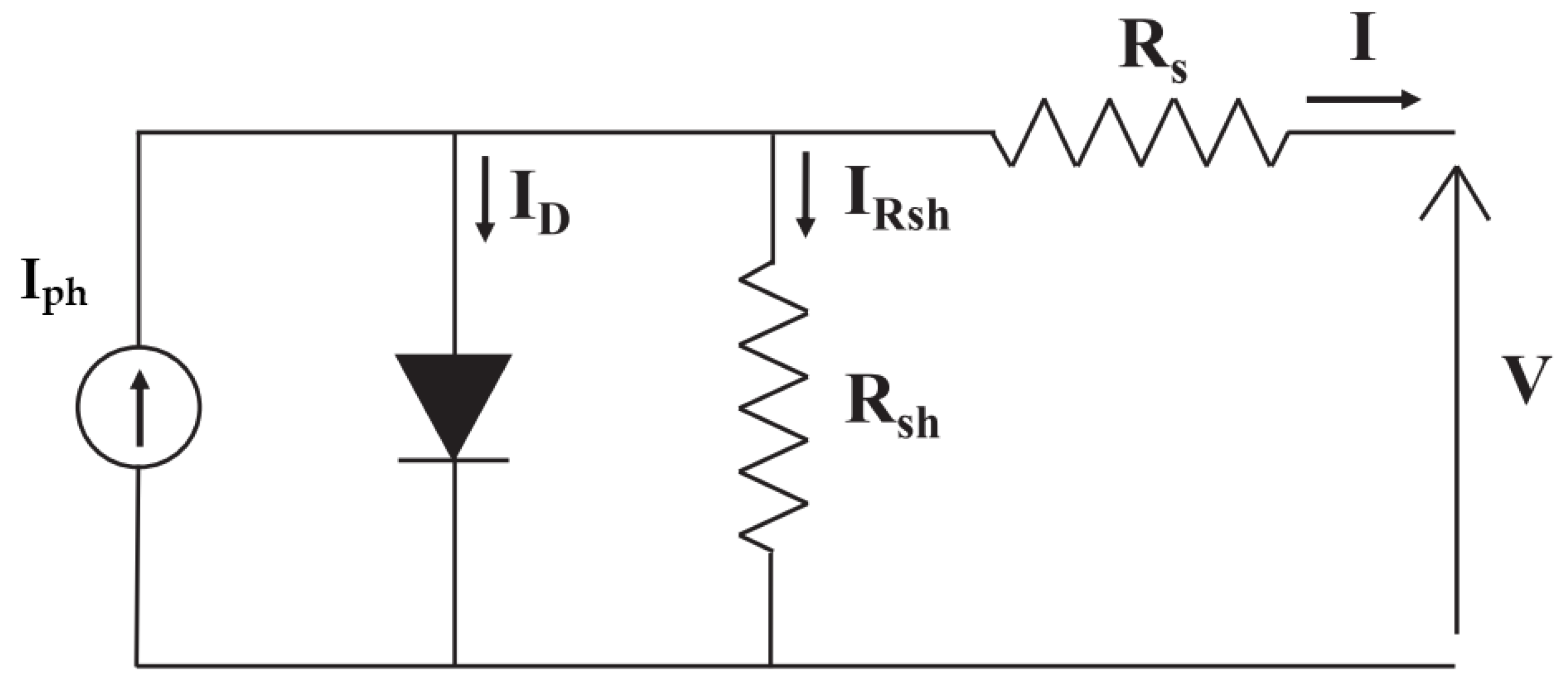
2.1. Single Diode Model

The single diode model is composed of a photocurrent-generated source I p h connected, in parallel, with a diode and two resistances, R s h and R s , as illustrated in Figure 1. The equation representing the voltage and current relationship is presented below:
I = I p h I d 1 I R s h = I p h I 0 e V + I R s a V T 1 V + I R s R s h
where I p h is the current generated by the solar irradiance, I 0 is the reverse saturation current, R s and R s h represent the series, and parallel resistances, respectively. Parameter a is the diode ideality factor, V T is the thermal voltage of the PV module having Ns cells connected in series, K is the Boltzmann constant ( 1.3806503 × 10 23 ) J/K, q is electron charge ( 1.60217646 × 10 19 ) C, and T is the temperature in K.
Based on the relationship of current and voltage described above, the following equations help illustrate the behavior of PV modules at the three remarkable points:
At the short circuit, V = 0 and I = I s c , and, drawing on Equation (1), we end up with the equation below:
I s c = I p h I 0 e I s c R s a V T 1 I s c R s R s h
Therefore,
I p h = I s c + I 0 e I s c R s a V T 1 + I s c R s R s h
At the open-circuit mode, I = 0 and V = V o c , and, drawing on Equation (1), we end up with the equation below:
0 = I p h I 0 e V o c a V T 1 V o c R s h
Therefore,
I p h = I 0 e V o c a V T 1 + V o c R s h
Combining Equations (5) and (3) we obtain:
I 0 = I s c + I s c R s R s h V o c R s h e V o c a V T e I s c R s a V T
Substituting Equation (6) into Equation (5) we find:
I p h = ( I s c + I s c R s R s h V o c R s h ) e V o c a V T 1 e V o c a V T e I s c R s a V T + V o c R s h
At the maximum power point, I = I m p , and V = V m p , and, drawing on Equation (1), we end up with the equation below:
I m p = I p h I 0 e V m p + I m p R s a V T 1 V m p + I m p R s R s h

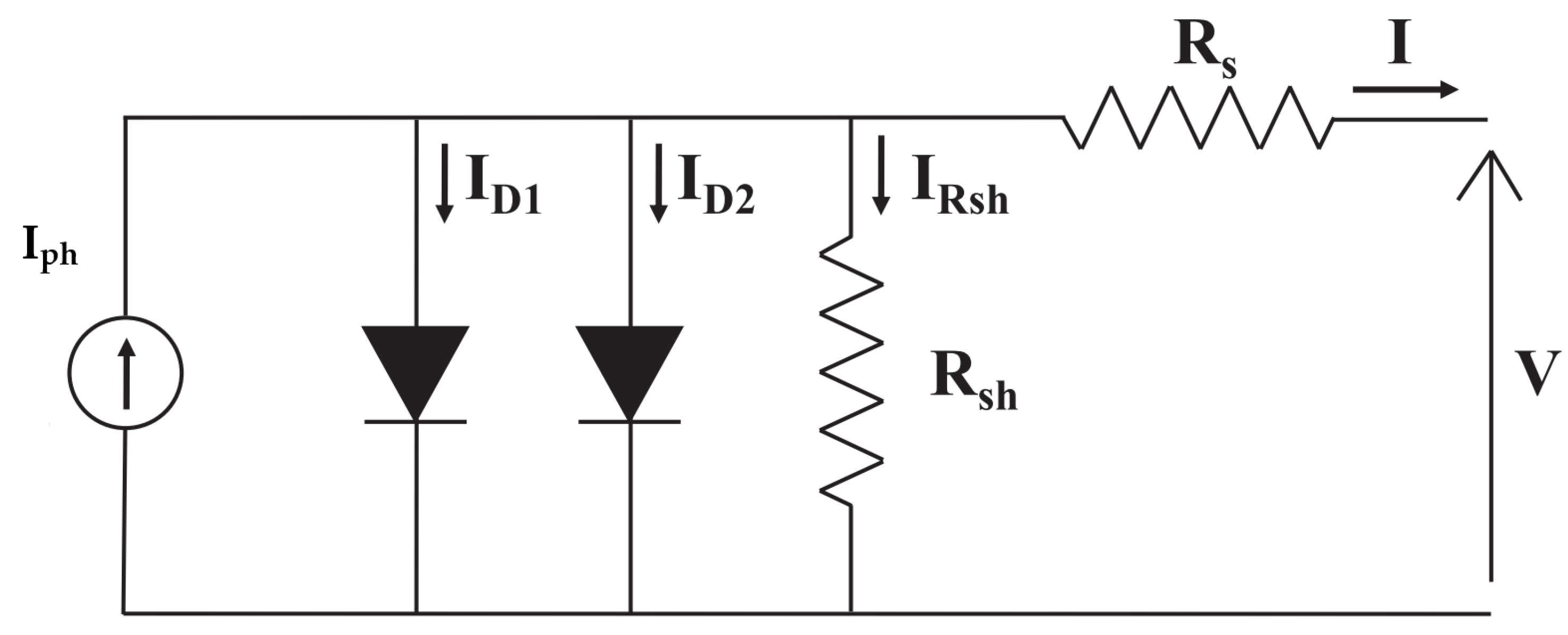
2.2. Double Diode Model

The single diode model naturally neglected the recombination loss in the forbidden region. The double diode model developed so as to overcome the gaps in the single diode model and, thereby, obtain an accurate solution. The electrical scheme, having the current–voltage relationship provided below, is represented in Figure 2:
I = I p h I d 1 I d 2 I R s h
I = I p h I 01 e V + I R s a 1 V T 1 I 02 e V + I R s a 2 V T 1 V + I R s R s h
where a 01 and a 02 are the ideality factors of the two diodes and I 01 and I 02 constitute their reverse saturation currents.
At the open circuit point, I = 0 and V = V o c , and, based on Equation (10), we obtain the equation below:
0 = I p h I 01 e V o c a 1 V T 1 I 02 e V o c a 2 V T 1 V o c R s h
Therefore,
I p h = I 01 e V o c a 1 V T 1 + I 02 e V o c a 2 V T 1 + V o c R s h
At the short circuit point, I = I s c and V = 0, and, based on Equation (10), we obtain the equation below:
I s c = I p h I 01 e I s c R s a 1 V T 1 I 02 e I s c R s a 2 V T 1 I s c R s R s h
Therefore,
I p h = I s c + I 01 e I s c R s a 1 V T 1 + I 02 e I s c R s a 2 V T 1 + I s c R s R s h
Using Equations (12) and (14) we obtain:
I 02 = I s c + I s c R s R s h V o c R s h I 01 e V o c a 1 V T e I s c R s a 1 V T e V o c a 2 V T e I s c R s a 2 V T
Substituting Equation (15) into Equation (12) we find:
I p h = I 01 e V o c a 1 V T 1 + I s c + I s c . R s R s h V o c R s h I 01 e V o c a 1 V T e I s c R s a 1 V T e V o c a 2 V T e I s c R s a 2 V T e V o c a 2 V T 1 1 + V o c R s h
At the maximum power point, I = I m p and V = V m p , and, therefore, from Equation (10) we obtain:
I m p = I p h I 01 e V m p + I m p R s a 1 V T 1 I 02 e V m p + I m p R s a 2 V T 1 V m p + I m p R s R s h

3. Implementation of FFO Algorithm

Flying foxes optimization (FFO) is a population-based stochastic algorithm that draws on different techniques used by flying foxes to survive in the event of high temperatures [23]. This method deploys a hybrid algorithm structure, mixing operators from existing algorithms [24,25,26]. The performance of FFO heavily depends on the size of the chosen population (N), replacement list ( R L ), and attraction constant (b). The steps involved in the FFO algorithm are described below.

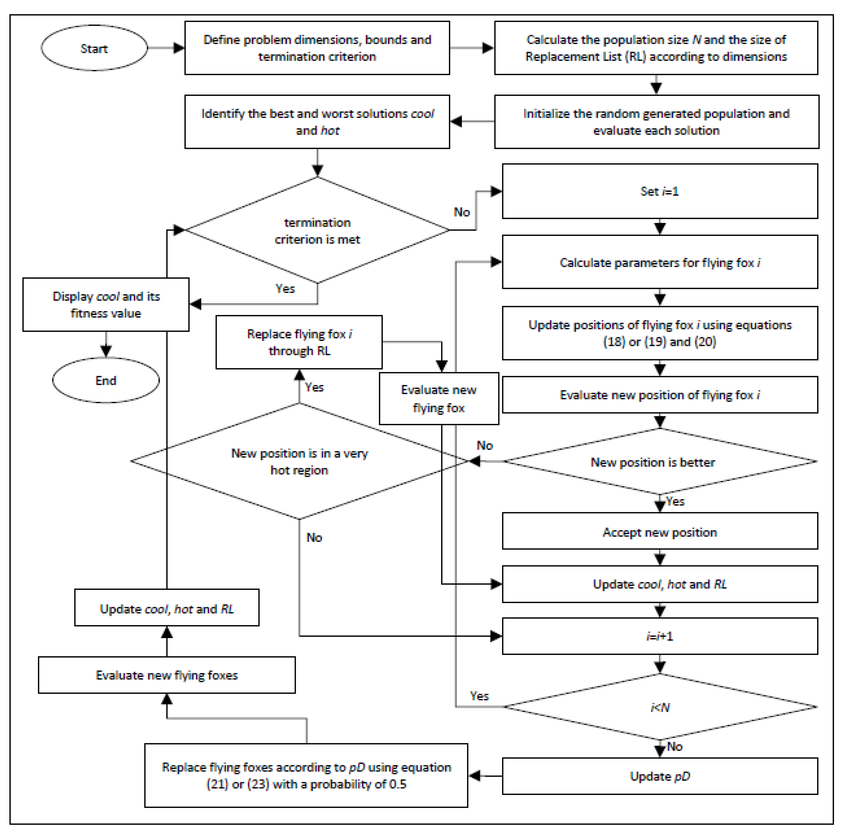
3.1. Functioning of Flying Foxes Algorithm

Flying foxes represent some of the largest bat species in existence. Their movements in space depend on their being observant of their environments since they cannot echolocate. After night meals, they come back to their habitat trees. Flying foxes seek cooler trees to rest upon so as to protect themselves from rising morning heatwaves. Most of the time, those that are first to locate a tree with an acceptable degree of heat are generally suffocated by other flying foxes and die [27].

3.2. The Application of FFO Algorithm

This new paradigmatic algorithm begins with an arbitrary set of several of the resulting positions of each flying fox. Such positions are illustrated through a vector, x = ( x 1 , . . . , x m ), that possesses m-dimensional elements. Next, the objective function evaluates the solutions for the positions mentioned earlier. Accordingly, flying foxes seek to locate a cooler tree in order to guarantee survival in the case of high temperatures.

3.2.1. Movement of Flying Foxes

Since flying foxes follow one another’s paths or look for the nearest tree, it could be presumed that if the habitat tree does not provide the convenient minimum temperature for the flying foxes, they move towards a different one to escape the intense heat. The formulation of this movement may be be illustrated by the equation below:
x i , j t + 1 = x i , j t + a · r a n d ( c o o l j x i , j t )
with x i 0 U (x m i n , x m a x ), x i , j t is the j-th constituent of FF(i), at reiteration t, a is a steady value, rand∼U(0,1) and cool corresponds to the location of the FF situated in the tree that has a minimum temperature. Equation (18) is deployed when |f(cool) −f(x i )| > δ 1 2 , where cool is the position vector of the flying fox situated in the coolest location ever discovered, which is the best solution ever found and the parameter δ 1 equates to the longest distance possible wherein two flying foxes are deemed near one another. When a flying fox approaches a tree with the lowest temperature (|(f(cool) −f(x i )| δ 1 2 ), it searches for the nearest space in order to avoid suffocation. The next equations explain the phenomenon further:
n x i , j t + 1 = x i , j t + r a n d 1 , j · ( c o o l j x i , j t ) + r a n d 2 , j · ( x R 1 j t x R 2 j t )
x i , j t + 1 = nx i , j t + 1 , i f j = k o r rnd j p a x i , j t , o t h e r w i s e
where rand∼U(0,1), r n d j is an arbitrary number between 0 and 1, x R 1 t and x R 2 t are two arbitrary members belonging to the current population and pa is a probability constant. Eventually, k, which is selected at random in {1,2,…,m}, and ensures that a minimum of one constituent from n x i , j t + 1 is chosen by x i , j t + 1 , to guarantee that there is no duplication between the original solution and the new one.
An assessment of the calculated solutions is undertaken. When the flying fox has found the tree with the lowest temperature, it is approved as a new solution. Otherwise, it comes back to the latest location.

3.2.2. Death and Replacement Flying Foxes

Various reasons lead to the deaths of flying foxes. For instance, they may end up in a region with intense heat, which is very remote, while looking for the coolest tree. In that case, they cannot escape death. As an alternative, a replacement List (RL) is resorted to with the N L ’s unique optimal solutions. An arbitrary integer n∈[2, NL] is, thus, created, and the location of a newly-generated flying fox can be referred to in the equation below:
x i , j t + 1 = k = 1 n R L k , j t n
where R L k t is the k-th FF on the RL during t reiteration. Equation (21) is geared towards maximizing the possibility of spotting an adequate region.
Flying foxes may also die from being suffocated by other population members. In this case, and before an iteration is finalized, a probability is determined, based on how many flying foxes are found in the regions with the lowest temperature. It can be illustrated as follows:
p D = n c 1 p o p u l a t i o n s i z e
where nc closely relates to the number of FF with a similar objective function to the optimal solution.

Crossover Process

Genetic crossover is utilized to facilitate the mating of two flying foxes. The initial step involves randomly selecting two parents from the population, ensuring they are not the same. This crossover process produces two offspring, which are generated as follows:
o f f s p r i n g 2 = L · R 2 + ( 1 L ) · R 2 o f f s p r i n g 1 = L · R 1 + ( 1 L ) · R 2
R 1 and R 2 are distinct members of the population selected randomly, and L is a randomly generated value falling within the range of 0 to 1.

3.2.3. Fuzzy Self–Tuning Method

A tuning method is undertaken to render the FFO algorithm unaffected by the initial parameter setting. The parameters are calculated using a fuzzy logic (FL) that is identical to the one deployed by Nobile et al. [22] and Tsafarakis et al. [28].

3.2.4. FFO Pseudo-Code

The pseudo-code of FFO is presented in Figure 3 below:

3.3. The Objective Function

The primary reason for the optimization is to estimate the PV module parameters. Indeed, its purpose is to produce solutions for the objective function that fulfil the data sheet inputs of the PV modules employed in this study. Such a goal is achieved using mathematical equations based on the remarkable points above. In the literature, some of the past studies validated only the maximum power point [29]. However, this paper formulated the objective function by adopting the three major points. Table 1 mentions the parameters that are optimized by adopting the proposed algorithm. Moreover, it points to the remaining parameters determined by deploying certain equations represented in Section 2 for single and double diode models.
Therefore, the Equations (1) and (10) are presented as follows:

3.3.1. Optimization Function of the Single Diode Model

Rewrite the three equations of a single diode model adopting the notation below: a = x 1 , R s = x 2 and R s h = x 3 .
Optimized function at short circuit (from Equation (2)):
f 1 = I s c I p h + I 0 e I s c x 2 x 1 V T 1 + I s c x 2 x 3
Optimized function at open-circuit (from Equation (4)):
f 2 = I p h I 0 e V o c x 1 V T 1 V o c x 3
Optimized function at maximum power point (from Equation (8)):
f 3 = I m p I p h + I 0 e V m p + I m p R s x 1 V T 1 + V m p + I m p x 2 x 3
The resulting optimization function is defined as the sum of the squared of the three optimized functions:
F = f 2 1 + f 2 2 + f 2 3

3.3.2. Optimization Function of the Double Diode Model

Rewrite the three equations of a double diode model adopting the notation below: a 1 = x 1 , a 2 = x 2 , R s = x 3 , R s h = x 4 and I 01 = x 5 .
Optimized function at open-circuit (from Equation (11)):
f 1 = I p h x 5 e V o c x 1 V T 1 I 02 e V o c x 2 V T 1 V o c x 4
Optimized function at short circuit point (from Equation (13)):
f 2 = I s c I p h + x 5 e I s c x 3 x 1 V T 1 + I 02 e I s c x 3 x 2 V T 1 + I s c x 3 x 4
Optimized function at MPP point (from Equation (17)):
f 3 = I m p I p h + x 5 e V m p + I m p x 3 x 1 V T 1 + I 02 e V m p + I m p x 3 x 2 V T 1 + V m p + I m p x 3 x 4
The resulting optimization function is defined as the sum of the squared of the three optimized functions:
F = f 2 1 + f 2 2 + f 2 3
We can see that function F has the same formulation for both models, while functions f 1 , f 2 and f 3 in Equations (27) and (31) are not the same because they are used for different models. Indeed, Equation (27) corresponds to the single diode model, while Equation (31) corresponds to the two diode model. Therefore, each equation’s specific functions and parameters vary depending on the model used.

4. Findings and Discussion

The algorithm (FFO) was implemented in this part to extract not only PV module parameters at STC but also at different temperatures and irradiations. This was achieved by deploying the expression of the short circuit I s c , the open voltage V o c , the maximum current ( I m p ), and the maximum voltage ( V m p ) as functions of temperature and irradiation [30,31]. The obtained parameters were then deployed to draw the I–V curves for the three variants of the PV modules. The following curves are compared to the experimental curves. At the end of this section, a comparison of the proposed algorithm with some prominent global metaheuristics algorithms is conducted to assess the FFO’s accuracy.

4.1. PV Module Input Data

The technical datasheet of the PV modules adopted in this study is provided in Table 2. It bears noting that all the data are given at STC, which means irradiance equaling 1000 w/m 2 , temperature of 25 C and a value of 1.5 for air mass.

4.2. Parameters under Distinct Weather Conditions

A PV module operates at different meteorological conditions of temperature and irradiation. For accurate modeling, it is significant to simultaneously compute the parameters of the single diode model at each environmental condition. Unlike other approaches [34] that require experimental I–V data, the proposed method necessitates only STC information in the technical datasheet of PV modules. Moreover, the suggested method does not rely on any analytical equation to determine the parameters at temperature and irradiance distinct from STC. However, the flying fox algorithm computes all the parameters at each variation of temperature and irradiation, deploying the following equations, which are from the study by Bogning Dongue et al. [32]:
Short-circuit current can be expressed as follows:
I s c = [ I s c , S T C + K i ( T T S T C ) ] ( G G S T C ) α
where K i is the thermal coefficient of short circuit current (A/ C), the exponent α is initiated to consider the nonlinearity behavior on which the short circuit current relies.
The open circuit voltage V o c may be represented as follows:
V o c = V o c , S T C 1 + β ln G S T C G ( T S T C T ) γ
where β is a coefficient with no dimensions, it depends on the technology of the PV module, and γ is the exponent that considers the voltage variation depending on temperature.
The current and voltage at MPP are represented by the equations below:
I m p = [ I m p , S T C + K i p ( T T S T C ) ] ( G G S T C ) α , V m p = V m p , S T C 1 + β ln G S T C G ( T S T C T ) γ
The constants α , β and γ correlate with significant reactions in the PV module (Table 3). They are experiment-based, and the exactness of the model relies heavily on the precision of the referenced calculation [30,31].

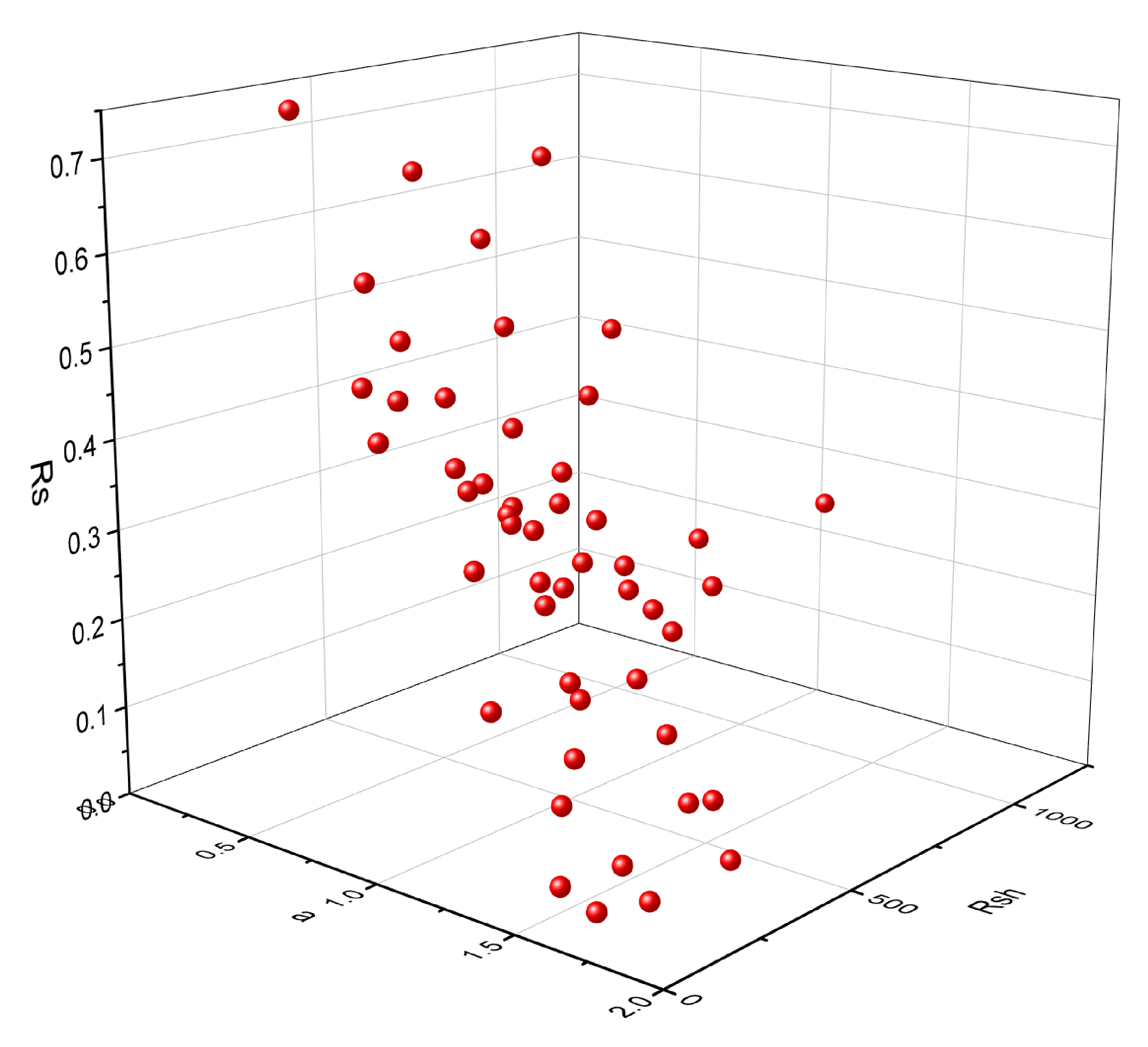
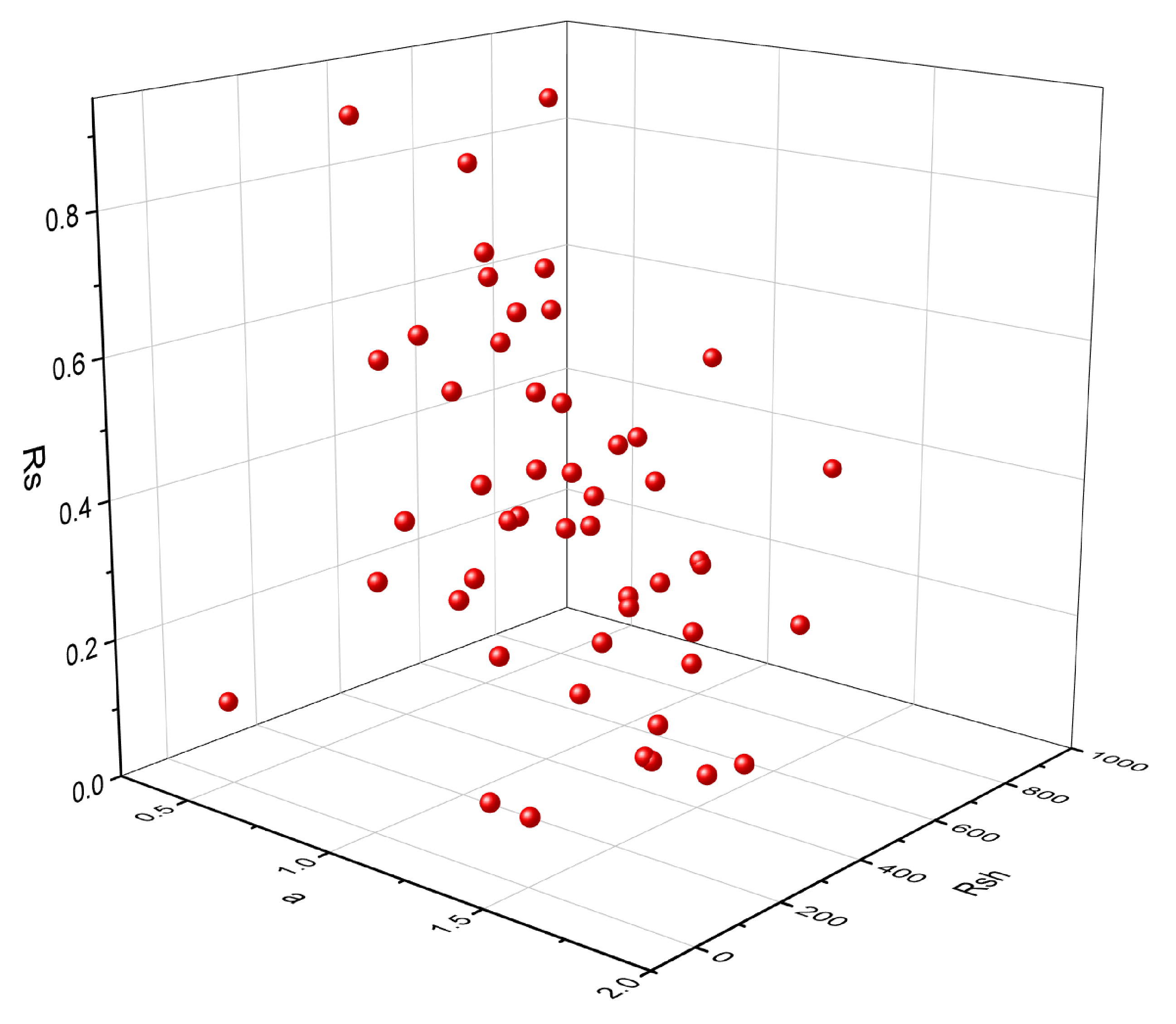
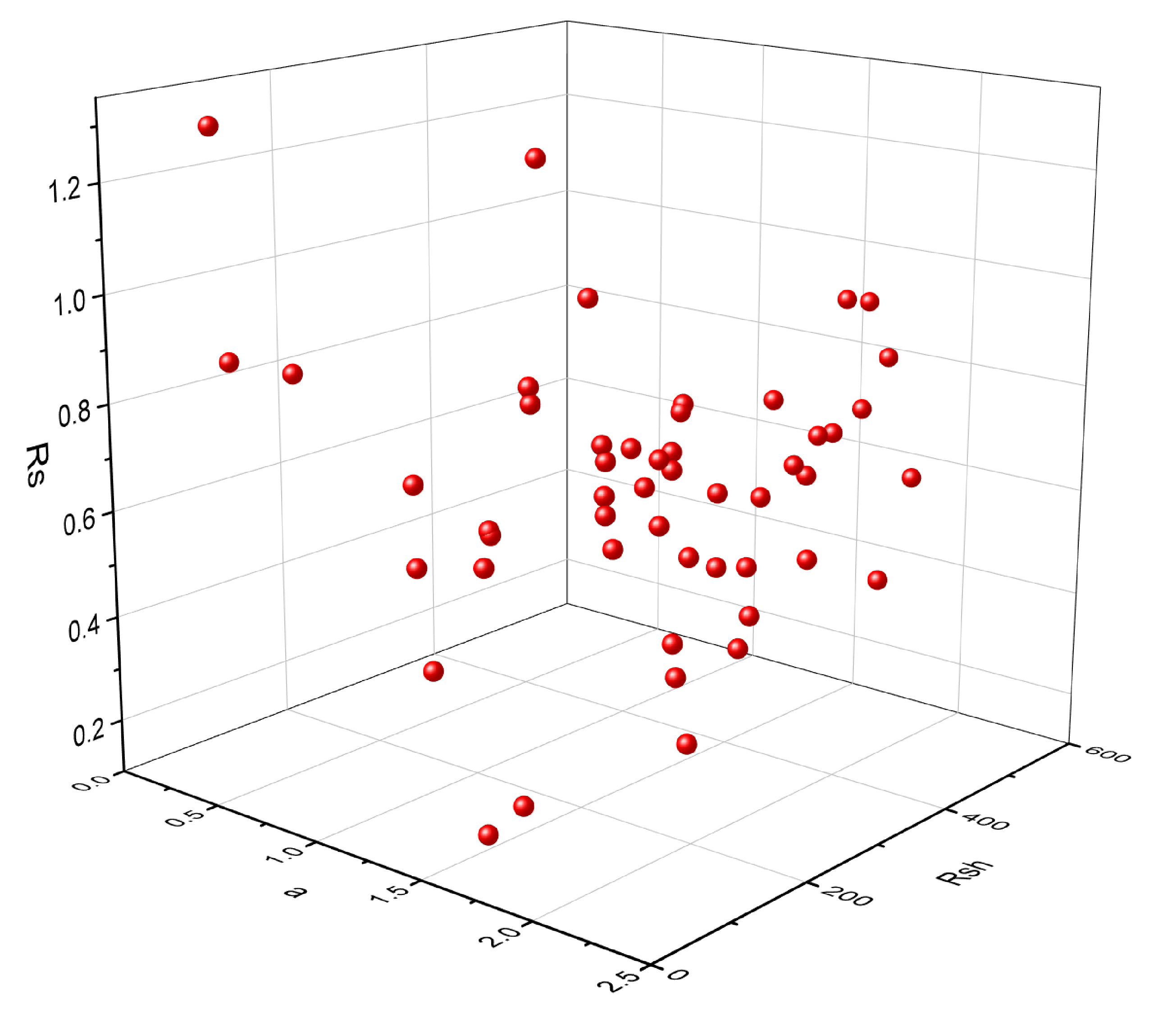
4.3. Parameter Determination of PV Module Adopting FFO

The implementation of FFO was carried out in MATLAB 2022. We considered a selected size of population (NP) superior to 15. The population size refers to the number of potential solutions or candidate solutions in the population at each iteration or generation. It represented the number of flying foxes being considered in the search for an optimal solution, and was a reasonable choice because the FFO algorithm performed better in this case [23]. The maximum number of fitness evaluations were 23,000 and 34,500 for single and double diode models. This could be attributed to the higher number of variables. The series resistance (R s ) was, in most cases, less than 1 Ω [35], unlike the shunt resistance (R s h ) that had much higher values. The ideality factor (a) was, overall, in the range 1 ⩽ a ⩽ 2 [35]. The user-defined inputs are summarized in Table 4. Deploying the above-mentioned objective function Equation (27) and the expressions of open voltage, short circuit, maximum voltage, and maximum current as a function of irradiance and temperature, the proposed algorithm was executed 10 times for every value of temperature and irradiation. The average values were, therefore, taken as the model parameters, presented in Table 5 and Table 6. Furthermore, the parameters were computed at every temperature and irradiation change.

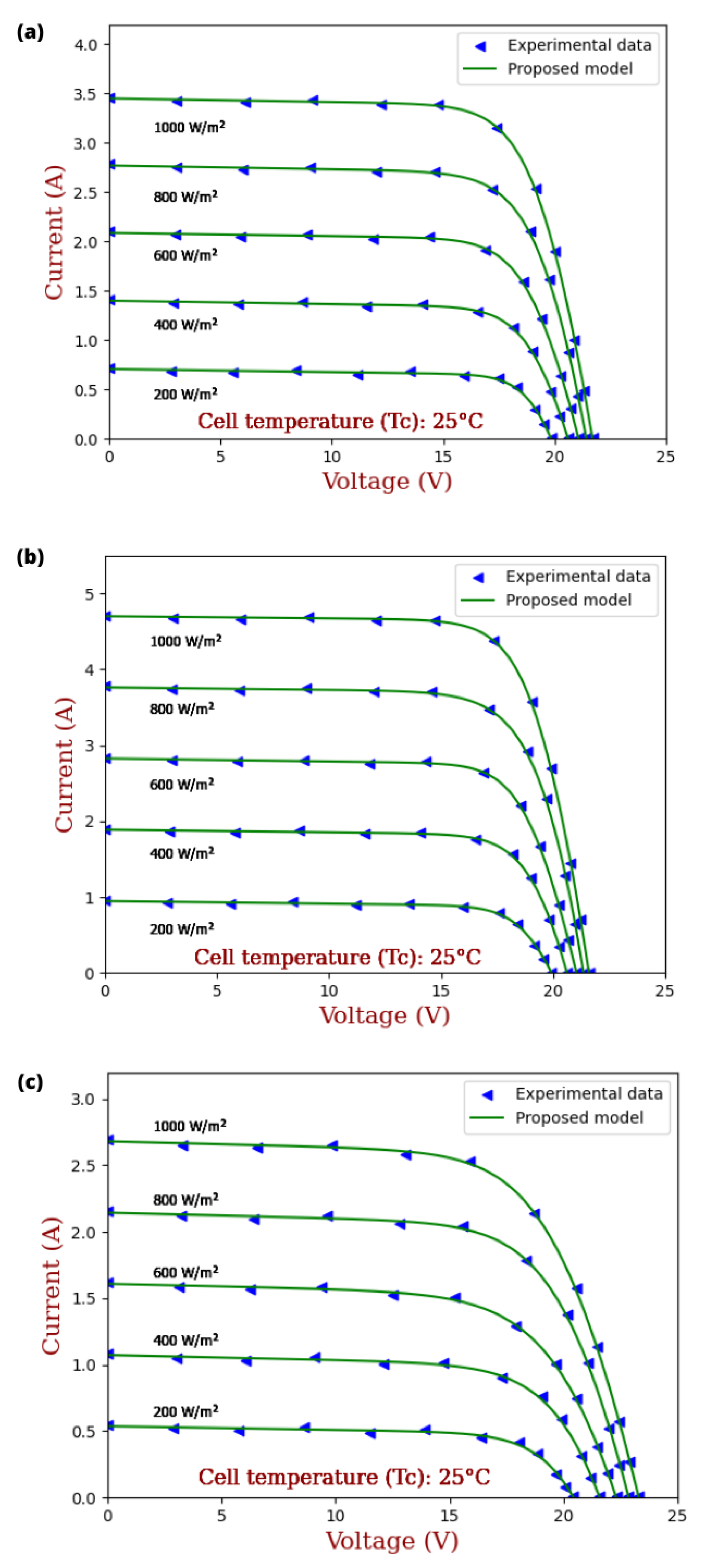
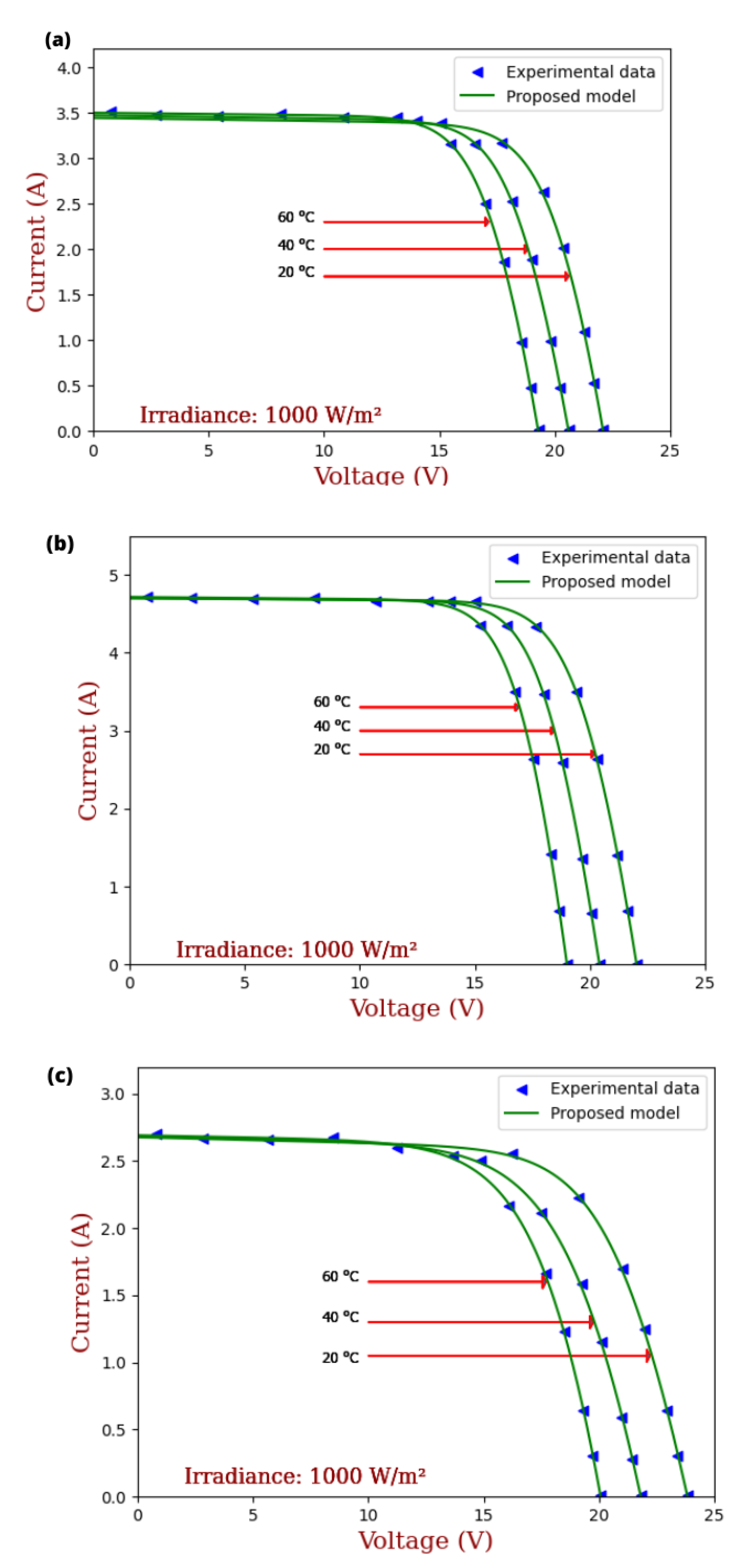
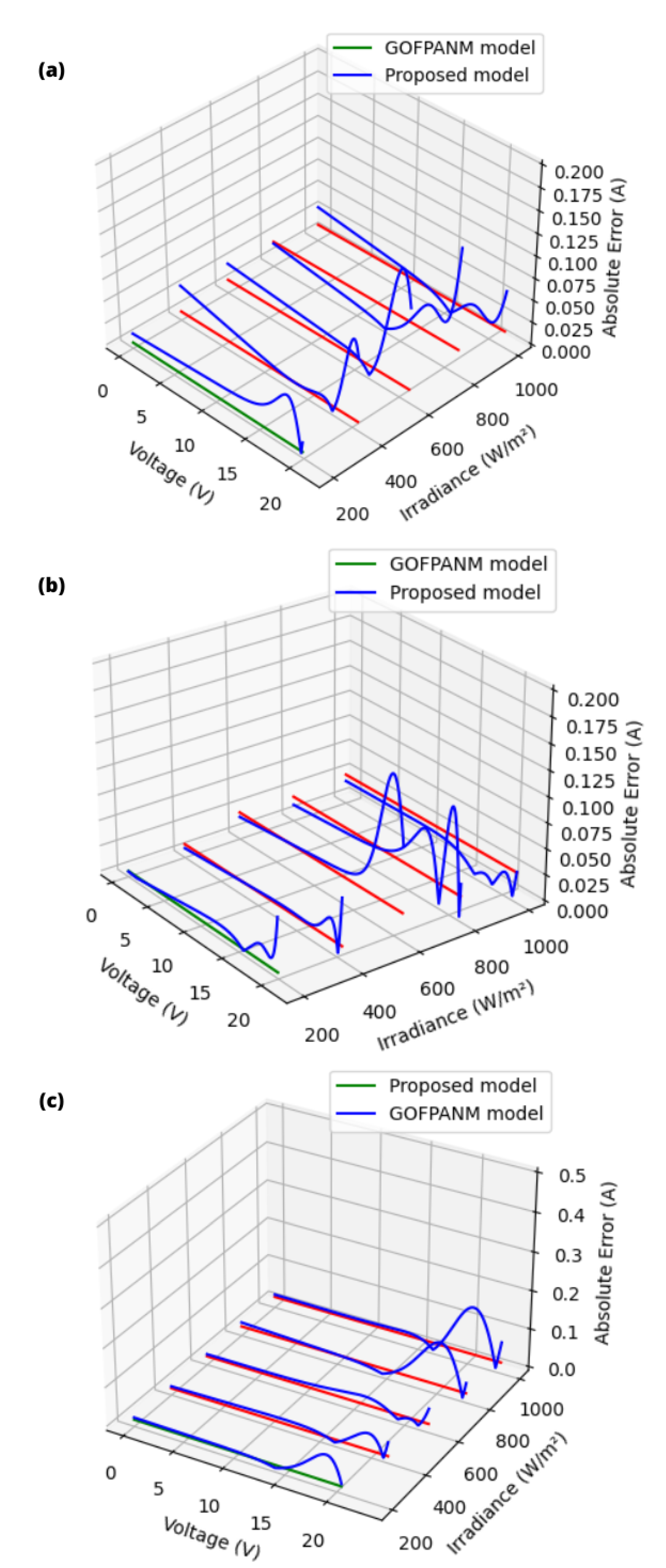
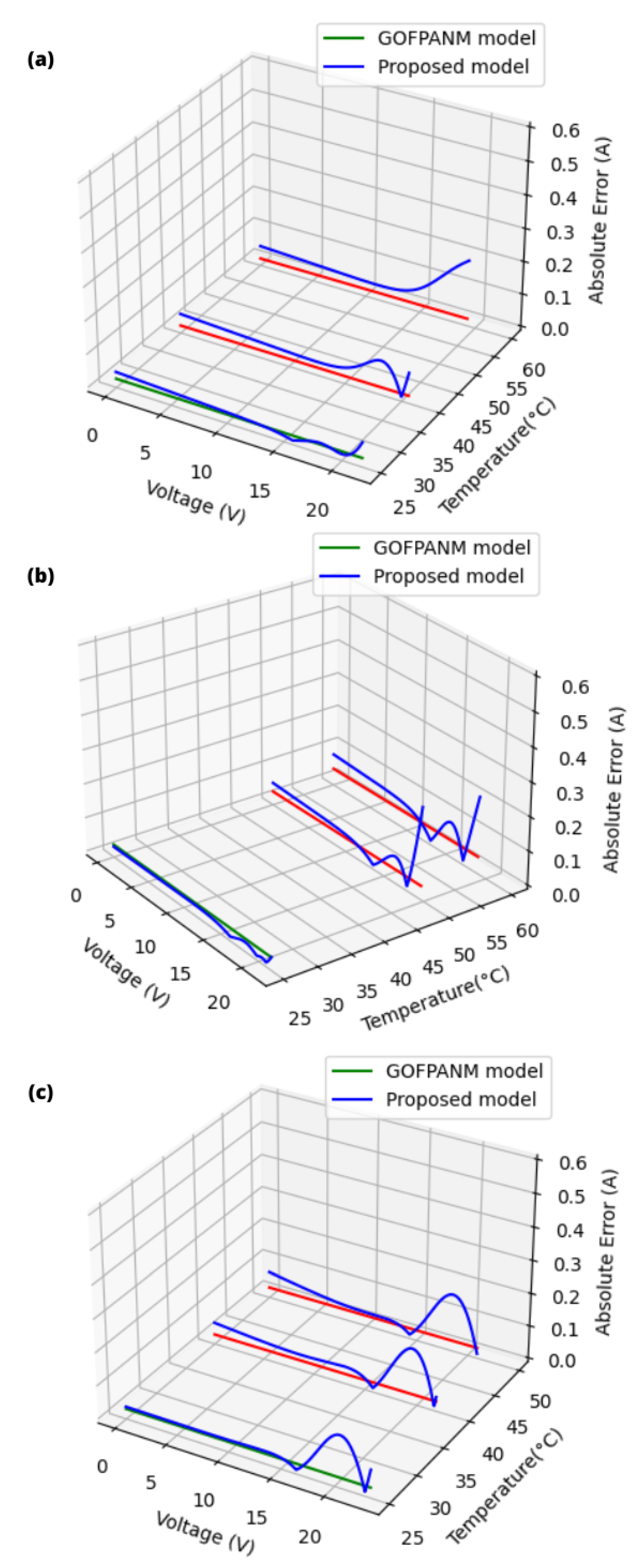
4.4. Empirical and Calculated I–V Characteristics of PV Module Adopting FFO

The steps to plot the I–V curves were carried out in Python using the function fsolve. The current and the voltage were computed for every coupled value (V, I), by substituting the resulting parameters in Equation (1) for a single diode model. Then, the voltage was incremented from the short circuit until the open circuit at each value of temperature and irradiation. The obtained charts for SM55, S75, and ST40 are presented in Figure 4a–c and Figure 5a–c. Based on Figure 4a–c, the accuracy was tested at different irradiations and a value of 25 C. The obtained I–V curves exhibited good congruity with the experimental data for the three modules. The accurateness of the adopted algorithm was also tested at three different temperatures: 20, 40 and 60 C. The irradiance level was fixed at 1000 w/m 2 . It can be gleaned from the I–V curves’ features that they closely corresponded with the empirical data. To better visualize the spread (scatter) of the three parameters (a, R s h , R s ) for each run, the algorithm was executed a total of 50 times, using a single diode model for three different modules (SM55, S75, and ST40). The results are presented in Table 7, Table 8 and Table 9, and scatter charts of the optimized parameters are shown in Figure 6, Figure 7 and Figure 8. It should be noted that each parameter could vary within a specific range of values. However, it is also noteworthy that each set of optimized parameters could achieve an objective function value of 0.
To quantify the exactness of the aforementioned method, the deviation of current, which may be referred to as the difference between the empirical and the computed current at every voltage point on the I–V curve, was calculated for different temperatures and irradiances. Figure 9a–c illustrate the deviation of the current of the SM 55, S75, and ST 40 modules derived at distinct levels of irradiance (200, 400, 600, 800 and 1000 W/m 2 ). The temperature was fixed at 25 C. By juxtaposing the deviation derived from [36], a slight difference in favor of the GOFPANM model was observed, particularly at high voltage, but the absolute deviation was kept below 0.14 A. A high level of deviation mostly happened near the MPP, all the more so since the series resistance value was a key player in defining the curvature of the I–V curve. Figure 10a–c illustrate the deviation of the current. The irradiation was set at 1000 W/m 2 , whereas the temperature was set at 25, 40, and 60 C for SM55 module, at 25, 50, and 60 C for S75 and 25, 40 and 50 C for ST40. The increase in temperature intensified the deviation for both techniques, notably at high voltage for all three modules. Concerning the multi-crystalline module, the deviation of the proposed method was particularly extreme at the lowest value of the series resistance ( R s ) . We introduced the RMSE (Root Mean Square Error) presented in Table 10. The Root Means Square Error (RMSE) was introduced to provide deeper assessment regarding the precision of the above-mentioned approach. The above metric measures the exactness and fitting of a computed, more thorough, evaluation of the accuracy of the above approach. In addition, this metric allowed us to evaluate the accuracy and adequacy of the calculated and experimental currents. It can be seen that the lower the value of the mean square error, the better the match between the calculated and empirical curves. The RMSE was computed as follows for different temperatures and irradiations:
RMSE = 1 M 1 M ( I m I e x ) 2
where M is the size of the chosen specimen; I e x and I m correspond to the empirical and computed currents, respectively. It is noticeable that the RMSE had a decreased value, except for high temperature, at which it attained 0.075.

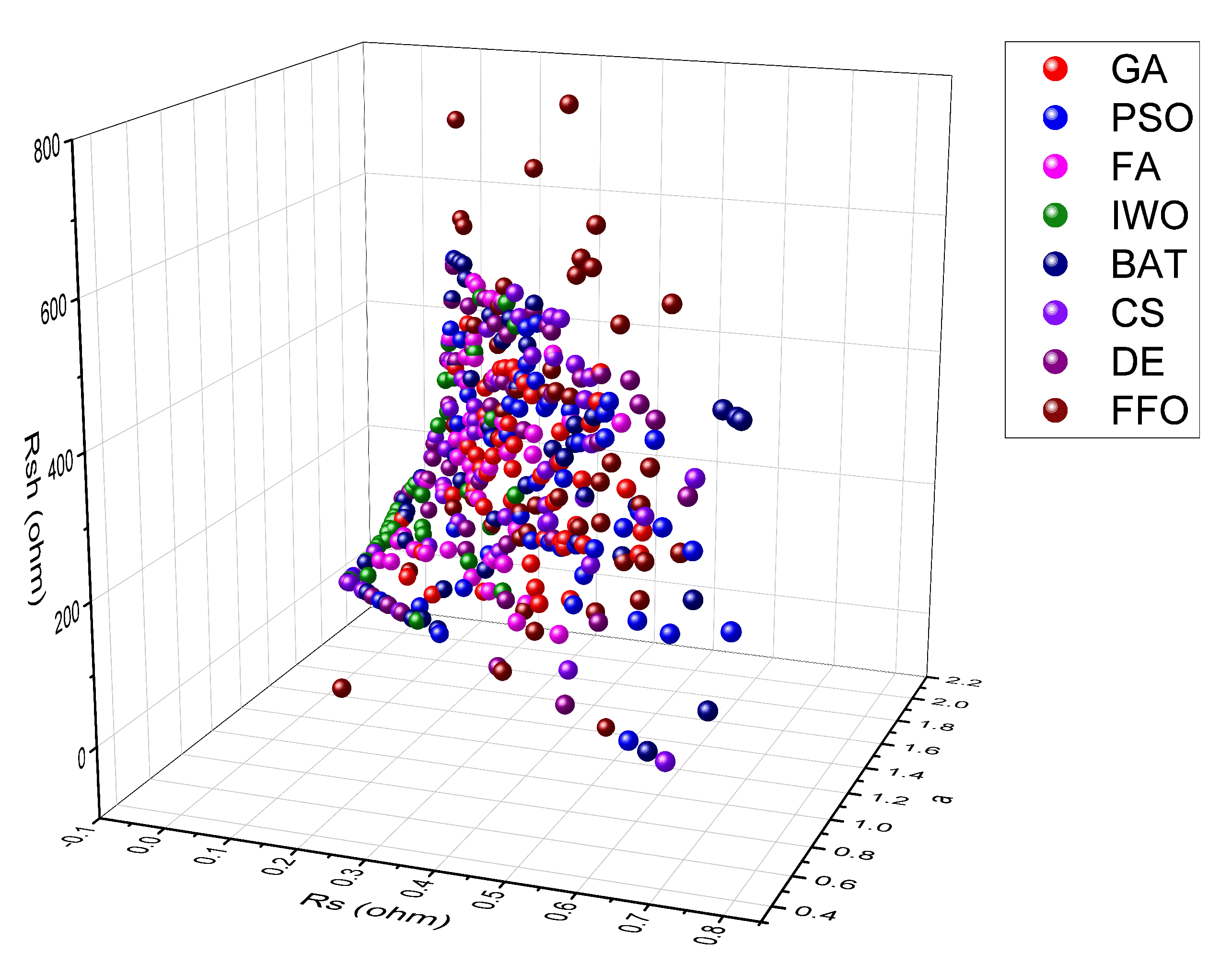
4.5. Comparative Study with Other Metaheuristics

To assess FFO’s accuracy and efficiency, its accuracy was juxtaposed with the following other prominent methods: Genetic algorithm (GA) [37], particle swarm optimization (PSO) [38], Invasive Weed Optimization (IWO) [39], Cuckoo Search (CS) [40], Differential Evolution (DE) [41], Bat Algorithm (BAT) [42] and Firefly Algorithm (FA) [43]. These metaheuristic optimization algorithms were adopted to resolve the objective functions of the single and double diode model Equations (27) and (31), respectively. The monocrystalline module SQ85 was adopted for parameter extraction. Table 11 lists the defined parameters selected for each algorithm. Every optimization algorithm was run 50 times for both models, and a statistical summary is presented in Table 12. Based on the data presented in Table 12, it can be observed that all eight optimization algorithms produced results with minimal error in all 50 runs. The FFO and DE algorithms had the worst outcomes, with errors around 10–11, but this level of inaccuracy would be insignificant in practical applications [23]. The optimized values of the cell parameters adopting the eight algorithms across all 50 trial runs, totaling 400 points, are illustrated in a 3D scatter plot in Figure 11. It can be concluded that, regardless of the algorithm used, it is possible to achieve the desired performance of the solar cell at significant points with various sets of cell parameters. The CPU time in Table 12 represents the duration taken to execute all 50 runs. It is noteworthy that BAT, CS, and FA algorithms performed faster than FFO, DE, and GA algorithms. Interestingly, the IWO algorithm produced more concentrated solutions with less spread, indicating its limited exploration capability compared to the other algorithms shown in Figure 11.

5. Conclusions

This paper discusses parameter extraction of photovoltaic (PV) modules using an emerging metaheuristic algorithm called flying foxes optimization (FFO). The strategies resorted to by flying foxes in the event of high temperatures led to the creation of the newly adopted population-related method. The primary aim of the adopted algorithm is to solve the objective function and determine the unknown parameters of PV modules by utilizing datasheet information at the three critical points of the I–V characteristics: open circuit, short circuit, and maximum power points. The study employed single and double diode models for various PV modules and presents detailed circuit analyses for both models. Some parameters were extracted by adopting the FFO algorithm, while the others were calculated analytically. To assess the accuracy of the proposed algorithm, a comparison was made between the computed curves and the experimental datasheet. The results indicated excellent correspondence. Furthermore, the absolute deviation and the RMSE (Root Mean Square Error) were computed and compared to the well-known GOFPANM model for the single diode model. The comparison showed a slight difference in favor of the GOFPANM model, especially at high voltages. However, the absolute deviation remained below 0.14 A. Moreover, the FFO algorithm was compared to other well-known metaheuristic optimizers. The results showed that, although it had a longer computational time than BAT, CS, and FA, its ability to optimize multiple parameters simultaneously resulted in a more efficient optimization process. This could lead to the development of a more accurate and efficient solar module. As technology and computing power advance, the FFO algorithm may become more appealing for PV module design. The positive outcomes achieved with the FFO optimizer highlight its potential value in the field of PV module design, particularly as optimization algorithms continue to be refined.

Author Contributions

Conceptualization, R.A. (Radouane Aalloul), A.E. and R.A. (Rahma Adhiri); Methodology, M.B. and R.A. (Rahma Adhiri); Software, R.A. (Radouane Aalloul); Validation, A.E. and R.A. (Rahma Adhiri); Investigation, M.B.; Writing—original draft, R.A. (Radouane Aalloul); Writing—review & editing, A.E., M.B. and R.A. (Rahma Adhiri). All authors have read and agreed to the published version of the manuscript.

Funding

This research received no external funding.

Data Availability Statement

The data presented in this study are available on request from the corresponding author. The data are not publicly available due to the data may involve confidential information of our research group.

Conflicts of Interest

The authors declare no conflict of interest.

Abbreviations

The following abbreviations are used in this manuscript:
STCStandard Test Conditions
FFOFlying foxes optimization
qElectron charge (1.60217646 × 10 19 C)
kBoltzmann constant (1.3806503 × 10 23 J/K)
TPV module temperature in Kelvin
V T Thermal voltage
aDiode ideality
I p h Light generated current of PV module
R s Series resistance of PV module
R s h Shunt resistance of PV module
N s Number of PV cells connected in series
I 0 Reverse saturation current of diode
I s c Short circuit
V o c Open voltage
I m p Maximum current
V m p Maximum voltage
MPPMaximum power point
K i Temperature Coefficient of I s c
K v Temperature Coefficient of V o c
GAGenetic Algorithm
PSOParticle Swarm Optimization
DEDifferential Evolution
IWOInvasive Weed Optimization
CSCuckoo Search
BATBat Algorithm
FAFirefly Algorithm
SDMSingle diode model
DDMDouble diode model
K I P , and  K V P Temperature coefficients for power

References

  1. Wang, K.; Yang, D.; Wu, C.; Shapter, J.; Priya, S. Mono-crystalline perovskite photovoltaics toward ultrahigh efficiency? Joule 2019, 3, 311–316. [Google Scholar] [CrossRef]
  2. Kalliojärvi-Viljakainen, H.; Lappalainen, K.; Valkealahti, S. A novel procedure for identifying the parameters of the single-diode model and the operating conditions of a photovoltaic module from measured current–voltage curves. Energy Rep. 2022, 8, 4633–4640. [Google Scholar] [CrossRef]
  3. Piliougine, M.; Guejia-Burbano, R.A.; Petrone, G.; Sánchez-Pacheco, F.J.; Mora-López, L.; Sidrach-de-Cardona, M. Parameters extraction of single diode model for degraded photovoltaic modules. Renew. Energy 2021, 164, 674–686. [Google Scholar] [CrossRef]
  4. Ruschel, C.S.; Gasparin, F.P.; Krenzinger, A. Experimental analysis of the single diode model parameters dependence on irradiance and temperature. Sol. Energy 2021, 217, 134–144. [Google Scholar] [CrossRef]
  5. Choulli, I.; Elyaqouti, M.; Saadaoui, D.; Lidaighbi, S.; Elhammoudy, A.; Obukhov, S.; Ibrahim, A. A Novel hybrid analytical/iterative method to extract the single-diode model’s parameters using Lambert’s W-function. Energy Convers. Manag. X 2023, 18, 100362. [Google Scholar] [CrossRef]
  6. Gholami, A.; Ameri, M.; Zandi, M.; Ghoachani, R.G. A single-diode model for photovoltaic panels in variable environmental conditions: Investigating dust impacts with experimental evaluation. Sustain. Energy Technol. Assess. 2021, 47, 101392. [Google Scholar] [CrossRef]
  7. Abbassi, A.; Gammoudi, R.; Dami, M.A.; Hasnaoui, O.; Jemli, M. An improved single-diode model parameters extraction at different operating conditions with a view to modeling a photovoltaic generator: A comparative study. Sol. Energy 2017, 155, 478–489. [Google Scholar] [CrossRef]
  8. Yahya-Khotbehsara, A.; Shahhoseini, A. A fast modeling of the double-diode model for PV modules using combined analytical and numerical approach. Sol. Energy 2018, 162, 403–409. [Google Scholar] [CrossRef]
  9. Sandrolini, L.; Artioli, M.; Reggiani, U.J.A.E. Numerical method for the extraction of photovoltaic module double-diode model parameters through cluster analysis. Appl. Energy 2010, 87, 442–451. [Google Scholar] [CrossRef]
  10. Chennoufi, K.; Ferfra, M.; Mokhlis, M. An accurate modelling of Photovoltaic modules based on two-diode model. Renew. Energy 2021, 167, 294–305. [Google Scholar] [CrossRef]
  11. Tifidat, K.; Maouhoub, N.; Benahmida, A.; Salah, F.E.A. An accurate approach for modeling IV characteristics of photovoltaic generators based on the two-diode model. Energy Convers. Manag. X 2022, 14, 100205. [Google Scholar]
  12. Gao, X.; Cui, Y.; Hu, J.; Xu, G.; Yu, Y. Lambert W-function based exact representation for double diode model of solar cells: Comparison on fitness and parameter extraction. Energy Convers. Manag. X 2016, 127, 443–460. [Google Scholar] [CrossRef]
  13. Ibrahim, H.; Anani, N. Evaluation of analytical methods for parameter extraction of PV modules. Energy Procedia 2017, 134, 69–78. [Google Scholar] [CrossRef]
  14. Wang, G.; Zhao, K.; Shi, J.; Chen, W.; Zhang, H.; Yang, X.; Zhao, Y. An iterative approach for modeling photovoltaic 386 modules without implicit equations. Appl. Energy 2017, 202, 189–198. [Google Scholar] [CrossRef]
  15. Nassar-Eddine, I.; Obbadi, A.; Errami, Y.; Agunaou, M. Parameter estimation of photovoltaic modules using iterative method and the Lambert W function: A comparative study. Energy Convers. Manag. X 2016, 119, 37–48. [Google Scholar] [CrossRef]
  16. Li, S.; Gong, W.; Gu, Q. A comprehensive survey on meta-heuristic algorithms for parameter extraction of photovoltaic models. Renew. Sustain. Energy Rev. 2021, 141, 110828. [Google Scholar] [CrossRef]
  17. Saadaoui, D.; Elyaqouti, M.; Assalaou, K.; Lidaighbi, S. Parameters optimization of solar PV cell/module using genetic algorithm based on non-uniform mutation. Energy Convers. Manag. X 2021, 12, 100129. [Google Scholar] [CrossRef]
  18. Devarapalli, R.; Rao, B.V.; Al-Durra, A. Optimal parameter assessment of solar photovoltaic module equivalent circuit using a novel enhanced hybrid GWO-SCA algorithm. Energy Rep. 2022, 8, 12282–12301. [Google Scholar] [CrossRef]
  19. Nayak, B.; Mohapatra, A.; Mohanty, K.B. Parameter estimation of single diode PV module based on GWO algorithm. Renew. Energy Focus 2019, 30, 1–12. [Google Scholar] [CrossRef]
  20. Kler, D.; Sharma, P.; Banerjee, A.; Rana, K.P.S.; Kumar, V. PV cell and module efficient parameters estimation using Evaporation Rate based Water Cycle Algorithm. Swarm Evol. Comput. 2017, 35, 93–110. [Google Scholar] [CrossRef]
  21. Farayola, A.M.; Sun, Y.; Ali, A. Global maximum power point tracking and cell parameter extraction in Photovoltaic systems using improved firefly algorithm. Energy Rep. 2022, 8, 162–186. [Google Scholar] [CrossRef]
  22. Nobile, M.S.; Cazzaniga, P.; Besozzi, D.; Colombo, R.; Mauri, G.; Pasi, G. Fuzzy Self-Tuning PSO: A settings-free algorithm for global optimization. Swarm Evol. Comput. 2018, 39, 70–85. [Google Scholar] [CrossRef]
  23. Zervoudakis, K.; Tsafarakis, S. A global optimizer inspired from the survival strategies of flying foxes. Eng. Comput. 2022, 1–34. [Google Scholar] [CrossRef]
  24. Liu, Z.; Jiang, P.; Wang, J.; Zhang, L. Ensemble forecasting system for short-term wind speed forecasting based on optimal sub-model selection and multi-objective version of mayfly optimization algorithm. Expert Syst. Appl. 2021, 177, 114974. [Google Scholar] [CrossRef]
  25. Kumar, S.; Tejani, G.G.; Mirjalili, S. Modified symbiotic organisms search for structural optimization. Eng. Comput. 2019, 35, 1269–1296. [Google Scholar] [CrossRef]
  26. Kumar, S.; Tejani, G.G.; Pholdee, N.; Bureerat, S. Multi-objective passing vehicle search algorithm for structure optimization. Expert Syst. Appl. 2021, 169, 114511. [Google Scholar] [CrossRef]
  27. Kumar, S.; Tejani, G.G.; Pholdee, N.; Bureerat, S. Multiobjecitve structural optimization using improved heat transfer search. Knowl. -Based Syst. 2021, 219, 106811. [Google Scholar] [CrossRef]
  28. Tsafarakis, S.; Zervoudakis, K.; Andronikidis, A.; Altsitsiadis, E. Fuzzy self-tuning differential evolution for optimal product line design. Eur. J. Oper. Res. 2020, 287, 1161–1169. [Google Scholar] [CrossRef]
  29. Benkercha, R.; Moulahoum, S.; Taghezouit, B. Extraction of the PV modules parameters with MPP estimation using the modified flower algorithm. Renew. Energy 2019, 143, 1698–1709. [Google Scholar] [CrossRef]
  30. Zhou, W.; Yang, H.; Fang, Z. A novel model for photovoltaic array performance prediction. Appl. Energy 2007, 84, 1187–1198. [Google Scholar] [CrossRef]
  31. Bogning Dongue, S.; Njomo, D.; Ebengai, L. An improved nonlinear five-point model for photovoltaic modules. Int. J. Photoenergy 2013, 2013, 680213. [Google Scholar] [CrossRef]
  32. Ishaque, K.; Salam, Z. An improved modeling method to determine the model parameters of photovoltaic (PV) modules using differential evolution (DE). Sol. Energy 2011, 85, 2349–2359. [Google Scholar] [CrossRef]
  33. Soon, J.J.; Low, K.S. Photovoltaic model identification using particle swarm optimization with inverse barrier constraint. IEEE Trans. Power Electron. 2012, 27, 3975–3983. [Google Scholar] [CrossRef]
  34. Kim, W.; Choi, W. A novel parameter extraction method for the one-diode solar cell model. Sol. Energy 2010, 84, 1008–1019. [Google Scholar] [CrossRef]
  35. Villalva, M.G.; Gazoli, J.R.; Ruppert Filho, E. Comprehensive approach to modeling and simulation of photovoltaic arrays. IEEE Trans. Power Electron. 2009, 24, 1198–1208. [Google Scholar] [CrossRef]
  36. Xu, S.; Wang, Y. Parameter estimation of photovoltaic modules using a hybrid flower pollination algorithm. Energy Convers. Manag. X 2017, 144, 53–68. [Google Scholar] [CrossRef]
  37. Holland, J.H. Adaptation in Natural and Artificial Systems: An Introductory Analysis with Applications to Biology, Control, and Artificial Intelligence; MIT Press: Cambridge, MA, USA, 1992. [Google Scholar]
  38. Kennedy, J.; Eberhart, R. Particle swarm optimization. In Proceedings of the ICNN’95-International Conference on Neural Networks, Perth, WA, Australia, 27 November–1 December 1995; Volume 4, pp. 1942–1948. [Google Scholar]
  39. Mehrabian, A.R.; Lucas, C. A novel numerical optimization algorithm inspired from weed colonization. Ecol. Inform. 2006, 1, 355–366. [Google Scholar] [CrossRef]
  40. Yang, X.S.; Deb, S. Cuckoo search via Lévy flights. In Proceedings of the 2009 World Congress on Nature Biologically Inspired Computing (NaBIC), Coimbatore, India, 9–11 December 2009; pp. 210–214. [Google Scholar]
  41. Storn, R.; Price, K. Differential evolution—A simple and efficient heuristic for global optimization over continuous spaces. J. Glob. Optim. 1997, 11, 341–359. [Google Scholar] [CrossRef]
  42. Yang, X.S. A new metaheuristic bat-inspired algorithm. In Nature Inspired Cooperative Strategies for Optimization (NICSO 2010); Springer: Berlin/Heidelberg, Germany, 2010; pp. 65–74. [Google Scholar]
  43. Yang, X.S. Nature-Inspired Metaheuristic Algorithms; Luniver Press: Frome, UK, 2010. [Google Scholar]
Figure 1. Electrical circuit of single diode model.
Energies 16 03531 g001
Figure 2. Electrical circuit of double diode model.
Energies 16 03531 g002
Figure 3. Flowchart of FFO algorithm [23].
Energies 16 03531 g003
Figure 4. The I–V curves for distinct irradiation levels (a) SM55, (b) S75 and (c) ST40.
Energies 16 03531 g004
Figure 5. The I–V curves for distinct temperature levels (a) SM55, (b) S75 and (c) ST40.
Energies 16 03531 g005
Figure 6. Optimized solutions (50 points) of the extracted parameters of multi-crystalline S75 using FFO Algorithm.
Energies 16 03531 g006
Figure 7. Optimized solutions (50 points) of the extracted parameters of mono-crystalline SM55 using FFO Algorithm.
Energies 16 03531 g007
Figure 8. Optimized solutions (50 points) of the extracted parameters of thin film ST 40 using FFO Algorithm.
Energies 16 03531 g008
Figure 9. The I-V curves for distinct irradiation levels (a) SM55, (b) S75 and (c) ST40.
Energies 16 03531 g009
Figure 10. The I-V curves for distinct temperature levels (a) SM55, (b) S75 and (c) ST40.
Energies 16 03531 g010
Figure 11. The dispersion best solutions for single diode model of the SQ85 cell adopting different algorithms.
Energies 16 03531 g011
Table 1. Summary of the optimized parameters for both single and double diode models.
ModelOptimized ParametersCalculated Parameters
Single diode modela, R s , R s h ( I p h ) , ( I 0 ) (6) and (7)
Double diode model a 1 , a 2 , R s , R s h , I 01 ( I p h ) , I 02 (15) and (16)
Table 2. Technical datasheet of PV modules adopted in this study.
ParameterMulti-CrystallineMono-CrystallineThin-Film
 S75 [32]SM55 [32]SQ85 [33]ST40 [32]
I s c (A)4.73.455.452.68
V o c (V)21.621.722.223.3
I m p (A)4.263.154.952.41
V m p (V)17.617.417.216.6
K v (mV/K)767672100
K i (mA/K)0.451.40.80.35
K v p (mV/K)767672.5100
K i p (mV/K)0.140.140.80.45
N s 36363642
Table 3. Constants estimation for PV modules.
Constant α β γ
Monocrystalline SM550.9840.0581.064
Multicrystalline S750.9960.0521.155
Thin-film ST400.9980.0871.343
Table 4. Input parameters for FFO algorithm.
ParametersSingle Diode ModuleDouble Diode Module
Decision Variables35
Lower BoundsLB = [0.5 0.001 50]LB = [0.5 0.001 50]
Upper BoundsUB = [2 1 1000]UB = [2 1 1000]
Number of Flying Foxes (Population size)20+2 D e c i s i o n V a r i a b l e s 20+2 D e c i s i o n V a r i a b l e s
Maximum no. of fitness evaluations23,00034,500
Table 5. Parameters for the proposed algorithm using single diode model at T = T S T C .
ParameterMono-Crystalline SM55Multi-Crystalline S75Thin Film ST40
G = 1000 W/m2   
a1.201.131.56
R s (ohm)0.410.290.77
R s h (ohm)278.39361.45236.53
G = 800 W/m2   
a1.281.391.51
R s (ohm)0.380.190.70
R s h (ohm)264.91316.59239.04
G = 600 W/m2   
a1.110.991.79
R s (ohm)0.610.480.66
R s h (ohm)321.72261.05258.40
G = 400 W/m2   
a1.041.071.49
R s (ohm)0.67
 
0.400.50
R s h (ohm)289.44295.92262.04
G = 200 W/m2   
a0.850.931.21
R s (ohm)0.720.740.66
R s h (ohm)331.82294.39361.43
Table 6. Parameters for the proposed algorithm using single diode model at G = G S T C .
ParameterMono-Crystalline SM55Multi-Crystalline S75Thin Film ST40
T = 20 °C   
a1.271.261.58
R s (ohm)0.340.290.63
R s h (ohm)296.75631.17236.77
T = 40 °C   
a1.101.011.86
R s (ohm)0.410.310.54
R s h (ohm)310.85381.23264.84
T = 60 °C   
a1.150.951.51
R s (ohm)0.470.360.36
R s h (ohm)398.29931.55317.01
Table 7. Optimized parameters of multi-crystalline S75 using single diode model.
Runa R s R sh Best CostRuna R s R sh Best Cost
11.60.04197.964.83 × 10 12 261.010.39267.712.29 × 10 13
20.950.43383.641.45 × 10 11 271.250.19115.851.60 × 10 12
31.40.19388.842.35 × 10 13 281.60.08371.043.80 × 10 14
41.090.35285.982.44 × 10 12 291.430.14200.413.43 × 10 12
50.640.6518.293.01 × 10 11 300.960.41228.876.00 × 10 12
61.110.34323.952.90 × 10 13 311.320.25656.045.86 × 10 14
71.710.02399.874.12 × 10 12 321.210.28328.637.38 × 10 12
81.240.29679.362.72 × 10 12 331.490.14394.582.80 × 10 14
91.360.22513.568.30 × 10 13 341.070.36288.212.47 × 10 13
100.350.75233.533.37 × 10 14 351.510.03109.591.49 × 10 12
111.230.29479.971.20 × 10 13 360.830.47181.941.49 × 10 14
121.340.2254.385.68 × 10 13 370.50.67438.326.89 × 10 13
130.750.53238.188.44 × 10 14 381.310.24495.091.48 × 10 14
140.950.44588.637.76 × 10 14 391.090.35404.881.18 × 10 12
150.850.49722.295.04 × 10 11 400.790.52473.557.76 × 10 11
161.190.3393.091.53 × 10 12 410.640.58221.741.23 × 10 11
171.140.33467.544.44 × 10 12 421.670.01214.511.21 × 10 13
181.060.36303.933.09 × 10 12 431.190.29287.811.63 × 10 11
190.840.44121.754.57 × 10 14 441.60.01135.032.49 × 10 11
201.370.19258.262.62 × 10 12 451.620.07423.685.94 × 10 16
211.260.281037.495.45 × 10 12 461.220.27276.022.53 × 10 13
220.530.66762.794.32 × 10 14 471.110.32178.542.44 × 10 14
231.450.1150.333.96 × 10 11 481.260.27462.672.27 × 10 12
240.770.49133.264.60 × 10 11 490.860.47274.231.08 × 10 11
251.010.38232.788.68 × 10 13 501.050.38443.683.22 × 10 15
Table 8. Optimized parameters of mono-crystalline SM55 using single diode model.
Runa R s R sh Best CostRuna R s R sh Best Cost
10.940.65373.851.44 × 10 13 260.970.4193.513.11 × 10 14
20.850.61123.542.48 × 10 13 271.240.25119.163.63 × 10 12
30.910.3273.413.22 × 10 13 281.380.30321.962.80 × 10 13
41.170.41192.505.08 × 10 11 291.510.21374.972.24 × 10 13
50.390.0957.921.78 × 10 16 301.650.09307.451.20 × 10 16
61.130.32107.173.61 × 10 15 311.390.31390.776.09 × 10 12
71.410.21181.361.60 × 10 11 321.670.09379.734.19 × 10 13
81.090.53374.393.38 × 10 14 331.390.32486.921.17 × 10 12
91.180.42208.991.16 × 10 12 340.890.64186.088.15 × 10 13
101.350.37875.802.61 × 10 12 350.960.64443.962.23 × 10 15
111.370.0598.051.19 × 10 11 361.550.22624.677.67 × 10 13
121.150.35125.671.49 × 10 12 371.120.54733.865.08 × 10 13
131.260.39315.971.29 × 10 12 380.640.89668.443.66 × 10 12
141.060.55335.571.89 × 10 15 391.560.13227.017.72 × 10 12
151.400.26243.523.38 × 10 13 400.710.83423.699.20 × 10 14
161.570.12233.831.72 × 10 13 411.390.29314.059.84 × 10 14
171.240.39272.551.80 × 10 11 420.880.69352.931.43 × 10 13
181.470.25405.824.80 × 10 13 431.180.45329.325.70 × 10 15
190.900.69473.136.31 × 10 13 441.260.42478.921.00 × 10 11
201.190.47487.842.20 × 10 13 450.980.57196.834.85 × 10 13
210.970.62315.958.16 × 10 11 461.180.47442.051.16 × 10 12
220.840.72368.312.18 × 10 13 471.230.42348.159.61 × 10 12
231.100.46177.967.66 × 10 12 481.400.32486.512.23 × 10 16
241.260.0684.042.14 × 10 13 491.150.47270.862.55 × 10 12
251.540.16268.167.50 × 10 12 500.580.91241.461.17 × 10 10
Table 9. Optimized parameters of thin film ST40 using single diode model.
Runa R s R sh Best CostRuna R s R sh Best Cost
11.790.81370.293.94 × 10 14 261.950.47187.685 × 10 13
21.780.74236.037.04 × 10 12 271.291.26199.517.79 × 10 12
31.650.2084.421.69 × 10 15 281.460.6795.171.46 × 10 12
41.920.68379.062.02 × 10 14 290.360.8860.601.13 × 10 15
52.030.49266.241.11 × 10 13 301.490.90137.293.04 × 10 15
61.900.66318.841.15 × 10 11 312.060.31174.891.57 × 10 13
71.460.6089.876.36 × 10 12 321.760.77241.444.47 × 10 14
81.520.1475.113.39 × 10 12 331.880.73409.038.45 × 10 13
91.710.79204.351.11 × 10 14 341.500.88135.255.57 × 10 16
101.710.72169.241.62 × 10 12 352.050.44244.781.56 × 10 12
111.860.69274.352.15 × 10 13 362.020.55347.724.78 × 10 16
121.730.83263.526.67 × 10 14 371.820.82532.717.50 × 10 16
132.000.62508.825.21 × 10 14 381.720.84268.642.89 × 10 13
141.880.73428.062.42 × 10 12 391.210.5972.183.76 × 10 13
151.680.77178.687.40 × 10 12 401.501.03208.002.29 × 10 12
161.730.69165.438.29 × 10 13 411.970.56279.424.58 × 10 15
171.730.92532.511.45 × 10 13 421.940.57249.003.72 × 10 16
181.710.94504.031.03 × 10 12 431.870.75474.811.34 × 10 13
191.750.76226.956.13 × 10 13 441.990.42182.013.47 × 10 14
201.190.7375.081.98 × 10 13 451.770.63163.554.87 × 10 13
211.290.4171.425.73 × 10 12 460.291.3060.192.39 × 10 12
221.890.70368.533.52 × 10 14 472.110.48422.581.69 × 10 14
231.660.80179.836.20 × 10 13 481.470.6695.381.06 × 10 13
241.820.66207.714.41 × 10 16 491.760.72205.465.75 × 10 13
250.680.8961.623.13 × 10 13 501.890.60225.771.29 × 10 12
Table 10. RMSE at distinct conditions.
Meteorological ParametersSM55S75ST40
T(°C)G(W/m²)RMSERMSERMSE
  Proposed
Model
GOFPANM
Model [36]
Proposed
Model
GOFPANM
Model [36]
Proposed
Model
GOFPANM
Model [36]
252000.0249252350.002511290.0097224370.001625720.027982870.00768238
254000.0300722350.006053170.0127951170.009334480.022887640.0078728
256000.0474386570.011178030.0558466160.02275590.02229860.01251004
258000.0325280.024818610.0368028980.020549060.048949410.01454162
2510000.0232631840.014645690.0163653610.025321460.055213820.01883885
4010000.0460210920.01080231--0.06496430.01749461
501000--0.059622890.028732360.07088910.01963535
6010000.072288930.009833440.0747379050.03827746--
Table 11. Input parameters of the eight distinct algorithms.
AlgorithmControl Parameter DescriptionSingle Diode ModelDouble Diode Model
Genetic Algorithm (GA)Mutation rate (µ)0.020.02
Crossover probability (CR)11
Population size (Np)5050
Maximum number of iterations10001500
Particle Swarm Optimization (PSO)Intertia Coefficient11
Damping Ratio of Inertia Coefficient0.990.99
Cognitive learning factor (c1)22
Social learning factor (c2)22
Population size (Np)5050
Maximum number of iterations10001500
Differential Evolution (DE)Maximum Number of Iterations10001500
Population Size5050
Crossover Probability0.20.2
Lower Bound of Scaling Factor0.20.2
Upper Bound of Scaling Factor0.80.8
Flying Foxes optimization (FFO)Number of Flying Foxes (Population Size)24.4724.47
parameter. Alpha[1 1.5 1.9][1 1.5 1.9]
parameter.pa[0.5 0.85 0.99][0.5 0.85 0.99]
function evaluation23,00034,500
Invasive Weed Optimization (IWO)Maximum Number of Iterations10001500
Initial Population Size1010
Maximum Population Size2525
Number of Seeds[0 5][0 5]
Variance Reduction Exponent22
Value of Standard Deviation[0.001 0.5][0.001 0.5]
Cuckoo Search (CS)Number of nests(or different solutions)2525
Discovery rate of alien eggs/solutions0.250.25
Maximum Number of Iterations10001500
Bat Algorithm (BAT)Population size2020
Maximum number of iterations10001500
Initial loudness11
initial pulse rate11
Firefly Algorithm (FA)Population size2020
Attractiveness constant11
Absorption coefficient0.010.01
Randomness reduction factor0.970.97
Maximum number of iterations10001500
Table 12. Summarized statistics of the case of SQ 85 adopting different algorithms.
PV modelAlgorithmBestAverageWorstStandard DeviationTotal CPU Time(s)
Shell SQ85
Single diode model
GA3.32 × 10−341.32 × 10−166.21 × 10−159.15 × 10−16142.9
PSO4.88 × 10−332.41 × 10−211.17 × 10−191.72 × 10−2085
DE8.64 × 10−151.69 × 10−111.35 × 10−102.66 × 10−11140.5
FFO3.31 × 10−161.60 × 10−111.40 × 10−102.94 × 10−11299.6
IWO2.00 × 10−196.73 × 10−147.45 × 10−131.39 × 10−1382.7
CS4.25 × 10−213.01 × 10−153.36 × 10−146.82 × 10−1531.9
BAT6.51 × 10−331.57 × 10−311.15 × 10−302.25 × 10−3116
FA6.33 × 10−323.41 × 10−304.25 × 10−296.75 × 10−3072.6
Shell SQ85
Double diode model
GA9.75 × 10−342.50 × 10−178.27 × 10−161.28 × 10−16179.15
PSO8.80 × 10−359.23 × 10−174.04 × 10−155.98 × 10−16123.15
DE2.05 × 10−175.64 × 10−131.50 × 10−112.23 × 10−12162.05
FFO1.12 × 10−171.35 × 10−111.71 × 10−103.57 × 10−11469.55
IWO2.26 × 10−202.20 × 10−131.97 × 10−123.50 × 10−13108.6
CS1.43 × 10−234.04 × 10−141.63 × 10−122.40 × 10−1340.65
BAT7.52 × 10−376.82 × 10−301.44 × 10−282.86 × 10−2918.25
FA5.40 × 10−349.82 × 10−321.88 × 10−302.78 × 10−31117.55
Disclaimer/Publisher’s Note: The statements, opinions and data contained in all publications are solely those of the individual author(s) and contributor(s) and not of MDPI and/or the editor(s). MDPI and/or the editor(s) disclaim responsibility for any injury to people or property resulting from any ideas, methods, instructions or products referred to in the content.

