Research on Solidity of Horizontal-Axis Tidal Current Turbine

Abstract

In this paper, the blade solidity of the tidal current turbine was investigated. Based on the blade element momentum theory, different design flow velocities were selected to design two blade types with different solidities. The geometric parameters of the blade were calculated using MATLAB programming, and the performance of two blades was compared in terms of the start-up flow rate, power generation and thrust by test experiment, which showed that the blade with higher solidity has better start-up performance and higher energy capture efficiency at low flow rates. The performance is better than that of the blade with low solidity, but due to the high solidity, the thrust is also high, which should be taken into account when installing the turbine.

1. Introduction

Tidal current energy is a clean, non-polluting, renewable energy source that does not affect the ecological balance. Research on tidal current turbine started in the mid-1970s, and now, it is mainly conducted in the United States, United Kingdom and other European countries to carry out high-power tidal current turbine experiments. As the tidal current turbine cause less ecological damage and has considerable economic benefits, many countries have followed suit, and a boom of tidal energy development has emerged.

Figure 1a shows a tidal current turbine designed and manufactured by Verdant Power, USA, with an advanced automatic convection system. When tidal flow velocity reaches 2.2 m/s, the generating power of the device can be up to 35.9 kW. The start-up flow velocity is 1 m/s. The innovation of the device is that it can automatically rotate at the best angle to capture more tidal current energy and improve the efficiency of the turbine according to the direction of the tidal current [1].

Figure 1b shows a 25 kW water turbine developed by Zhejiang University, China. The diameter of the device is 4.4 m, the design speed is 45 rpm, and the design flow velocity is 2.2 m/s. A sea trial experiment was successfully conducted, and the blade efficiency was around 24%, when the tidal flow rate reached the design flow rate of 2.2 m/s, which verified the effectiveness and correctness of the design method [2].

Although various forms of tidal energy harvesting devices have been proposed as conceptual designs, tidal energy generation devices that have reached commercial operation conditions are mainly horizontal-axis tidal turbines. The main drawbacks of vertical-axis turbines are their weak self-starting capability, large torque fluctuations during one rotation cycle and low energy conversion efficiency. Based on economic and technical difficulty considerations, the horizontal-axis turbine scheme is more suitable for large tidal power generation units exceeding 500 kW.

After rapid development in recent decades, the horizontal-axis tidal turbine has reached megawatt-level power generation and is considered the most promising tidal power generation technology for large-scale application, and some horizontal-axis tidal power generation devices have entered the final verification stage before commercial operation. The application of these projects will lay a good foundation for further development of tidal energy resources. The development of tidal energy resources is still at the initial stage, and most of the projects are still at the experimental demonstration stage. Although various novel designs of energy capture devices have been proposed, a more mature horizontal-axis turbine scheme is still the main application in the projects that have reached commercial operation. Currently, the UK and France are the international leaders in the development and application of tidal-wave energy resources.

At present, there are two main types of tidal power generation devices: a fixed type and a floating type. A fixed tidal power generation device relies on its own gravity, or through the conduit frame and other forms of support structure, to be fixed to the seabed, entirely submerged in the water. Although it is not affected by the surface conditions, it is more expensive to install and maintain, and it is not movable. Due to the proximity to the seabed, the tidal current flow slows down, limiting the performance of the turbine. With respect to the floating type, the turbine is fixed on a floating carrier and secured to the seabed by a mooring system. With a floating structure design, it can adapt to a wide range of water depths, has no special requirements for the topography of the seabed and is easy to install and maintain. It is easy to obtain more energy due to the fast surface flow. At present, the development of a floating tidal energy generation device will become a trend in tidal energy development. At present, most of the design of the tidal current turbine is based on the design theory of wind power blade. The shape of the designed blade is slender, and the solidity is low. However, the tidal energy is different from the wind energy, the flow velocity of the tidal energy is low, and the density of a fluid medium is high—an important parameter of different blades having a great impact on the efficiency of energy capture. Thus, this paper has studied the design of blade solidity.

2. Key Parameters of Blade Design

2.1. Solidity of blade

As shown in Figure 2a,b, there are two different solidities of tidal current turbines, which greatly affect the efficiency of energy capture. This is closely related to the design flow velocity, design blade speed and blade tip speed ratio.

Based on the momentum theory, when assuming that the blades could produce power without rotation, the axial force ($dF$) can be obtained using the following equation:

$$dF=4a\left(1-a\right)\rho V^2\pi rdr$$

(1)

where $\rho$ is the seawater density, $V$is the sea velocity far up stream, $a$ is the axial induction factor, and $r$ is he distance of the element from the hub.

Figure 3 shows the force analysis situation of the blade element. The value $a$ is the axial induction factor. The value $b$ is the tangential induction factor. $V(1-a)$ is the axial velocity of the seawater. The value $\mathsf{\Omega }r\left(1+b\right)$ is the tangential velocity. $W$ is the resultant velocity of the axial and tangential velocities.

$$W=\sqrt{{\left[V\left(1-a\right)\right]}^2+{\left[\mathsf{\Omega }r\left(1+b\right)\right]}^2}$$

(2)

The inflow angle is $\varnothing$, $\alpha$ is the angle of attack, and $\beta$ is the pitch angle [4].

$$\varnothing =arctan\frac{V\left(1-a\right)}{\mathsf{\Omega }r\left(1+b\right)}$$

(3)

Two forces that act on the blade element are the lifting and resisting forces:

$$d{F}_L=\frac{1}{2}\rho c{W}^2{C}_{L}dr$$

(4)

$$d{F}_D=\frac{1}{2}\rho c{W}^2{C}_{D}dr$$

(5)

where $c$ is the blade element’s chord length, $C_l$ is the lift coefficient, and $C_d$ is the resistance coefficient. From the blade element theory, the axial forces $dF$ and thrust forces $dT$ can be represented as follows:

$$dF=d{F}_{L}cos\varphi +d{F}_{D}sin\varphi =\frac{1}{2}B\rho c{W}^2\left(C_{L}cos\varphi +C_{D}sin\varphi \right)dr$$

(6)

$$dT=d{F}_{L}sin\varphi -d{F}_{D}cos\varphi =\frac{1}{2}B\rho c{W}^2\left(C_{L}sin\varphi -C_{D}cos\varphi \right)dr$$

(7)

Solidity $\sigma$ refers to the ratio of the blade projection and the swept area of turbine, which is expressed as [5]:

$$\sigma =\frac{{{\displaystyle \int }}_0^{R}B{C}_{r}dr}{\pi R^2}$$

(8)

where $B$ is the number of blades, $C_r$ is the chord length of the blade element at the radius$r$, and $R$ is the blade radius. Therefore, the solidity of a microblade element can be expressed as follows:

$$d\sigma =\frac{B{C}_r}{2\pi r}dr$$

(9)

The blade solidity can be obtained by equating Formula (1) with Formula (6):

$$\sigma ={{\displaystyle \int }}_0^R\frac{4asi{n}^2\varphi }{\left(1-a\right)\left(C_{L}cos\varphi +C_{D}sin\varphi \right)}dr$$

(10)

According to Formulas (3) and (10), the relation between blade solidity $\sigma$, sea velocity $V$, blade angle speed $\mathsf{\Omega }$ and axial inducer$\mathrm{a}$can be obtained. The calculation of these parameters is a key to blade design.

2.2. Number of Blades

Generally speaking, the number of blades depends on the tip speed ratio of the blade. The national standard (GB/T 13981-1992) gives the correspondence between the tip speed ratio and the number of blades.

Table 1. Tip speed ratio and the matching number of blades [6].

Tip Speed Ratio	Number of Blades
1	8~24
2	6~12
3	3~8
4	3~5
5~8	2~4
9~15	2~3

shows the number of blades corresponding to different tip speed ratios [5].

2.3. Blade Diameter

The blade diameter estimation equation is as follows:

$$D=\sqrt{\frac{8P}{\rho v^3\pi C_p{\eta }_1{\eta }_2}}$$

(11)

where $D$ is the blade diameter, $\mathrm{m}$; $P$ is the design output power of the blade, $W$; $\rho$ is the seawater solidity, $\mathrm{kg}/{\mathrm{m}}^3$; $v$ is the seawater flow velocity, $\mathrm{m}/\mathrm{s}$; $C_p$ is the energy capture coefficient, generally 0.30~0.40; ${\eta }_{1 }$ is the efficiency of the drive system; and ${\eta }_2$ is the efficiency of the generator.

Since the diameter of the blade is basically limited by the size of the blade installation platform, considering various factors such as the depth of the tidal current flow and installation and maintenance convenience. Therefore, the actual working environment of the blade should also be considered when determining the blade diameter using the above calculation method.

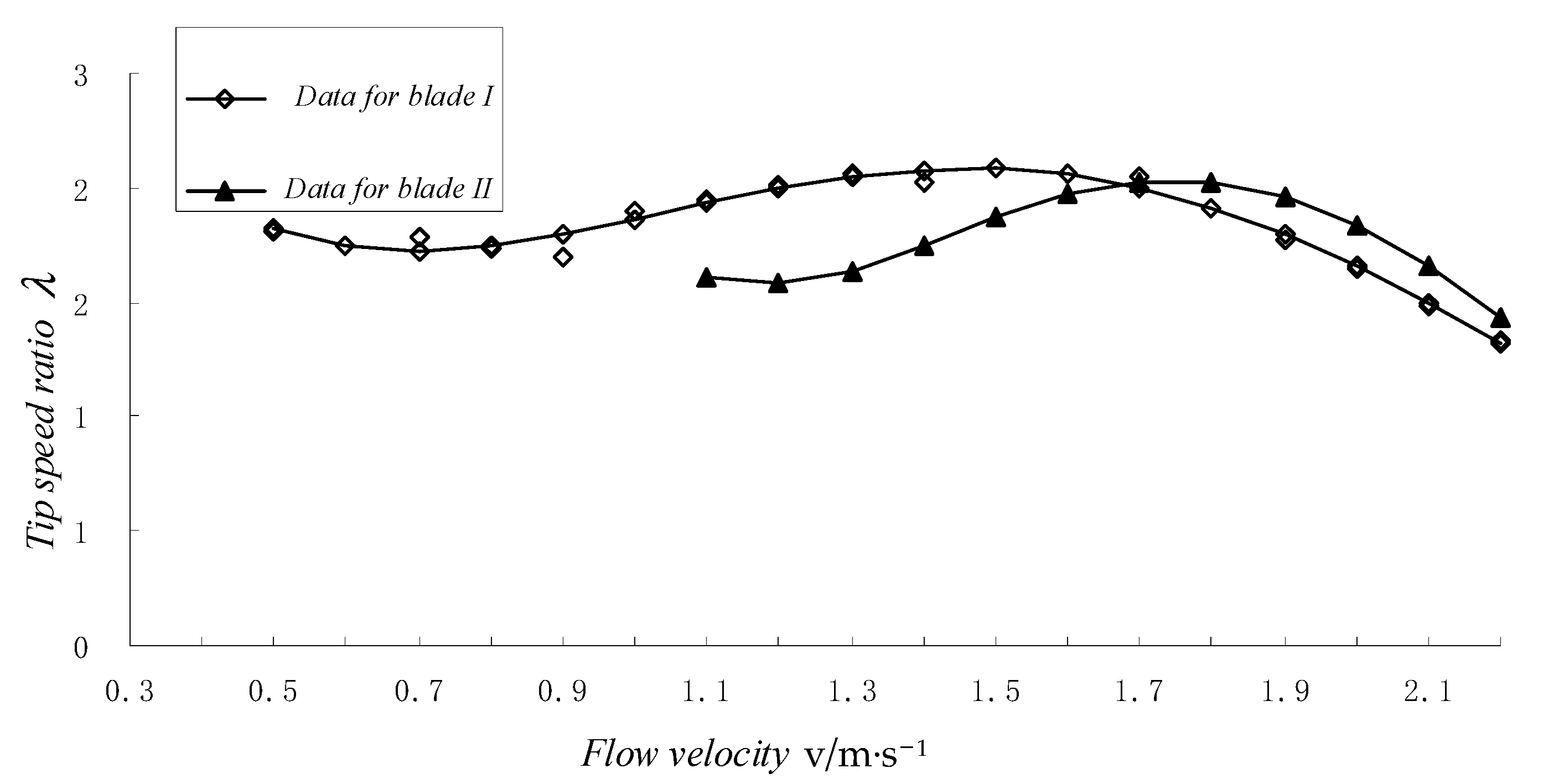
2.4. Tip Speed Ratio

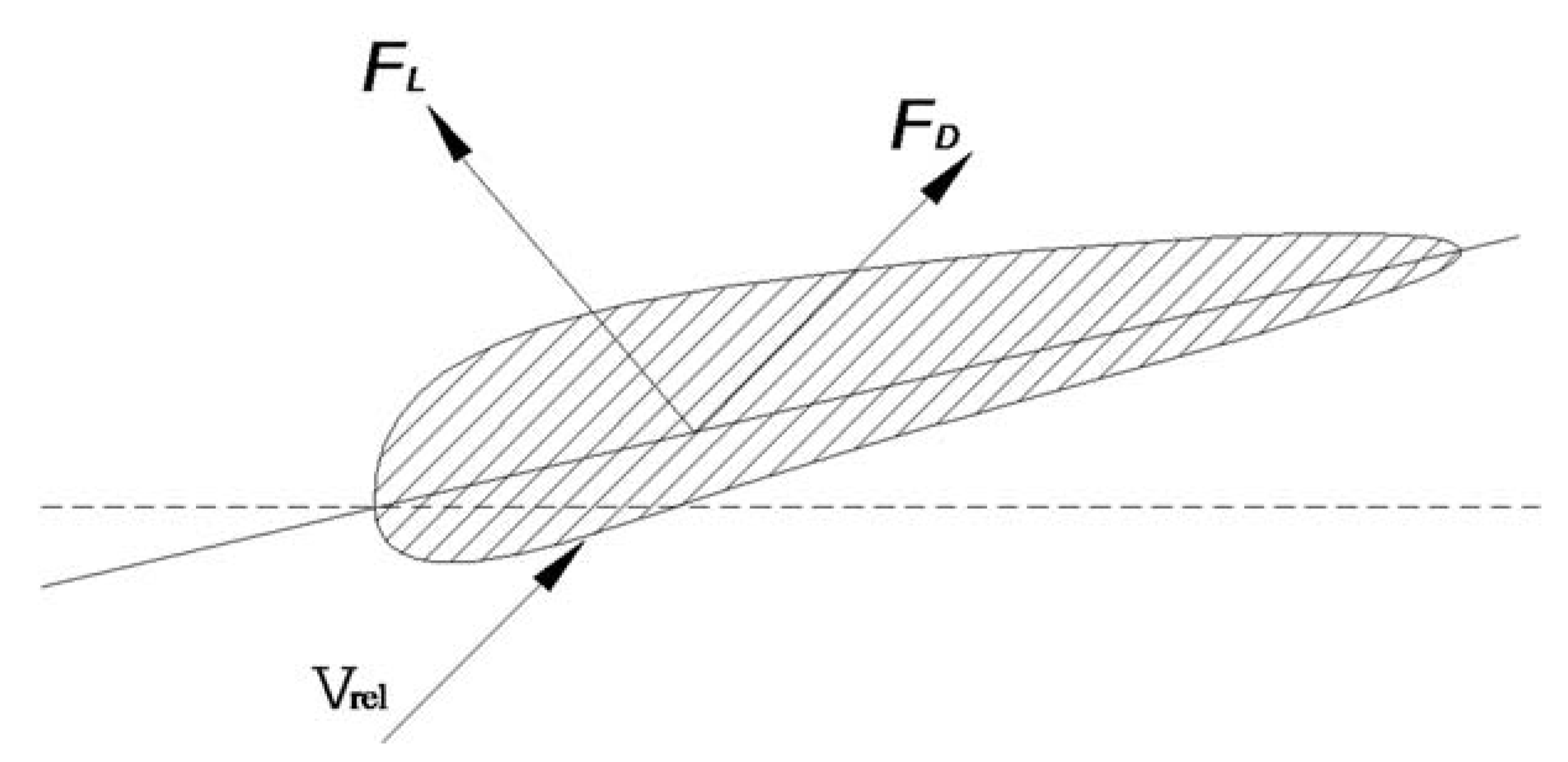
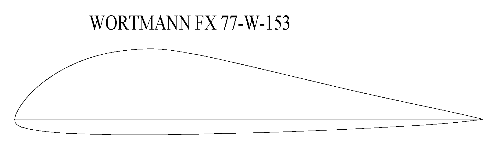
The ratio of blade tip linear velocity to tide velocity is called the tip speed ratio and can be expressed as follows:

$$\lambda =\frac{\omega R}{V}=\frac{\pi nR}{30V}$$

(12)

where $\omega$ is the rotational angular velocity, $\mathrm{rad}/\mathrm{s}$; $R$ is the blade radius, m; $n$ is the blade speed, and $\mathrm{r}/\min$; $V$ is the tide flow velocity, $\mathrm{m}/\mathrm{s}$.

The maximum energy capture efficiency of the water turbine appears near the optimum tip speed ratio. Moreover, blade $C_p$ is a function of tip speed ratio $\lambda$ and the pitch angle $\beta$. The capture power of the blade is determined by these two parameters. Since the pitch angle of the blade with a fixed pitch cannot be changed, selecting a suitable tip speed ratio will enable the turbine to capture the peak power [6].

2.5. Airfoil

The airfoil is the cross-sectional shape of the blade. The geometric parameters of the airfoil are mainly as follows [7]:

(1)

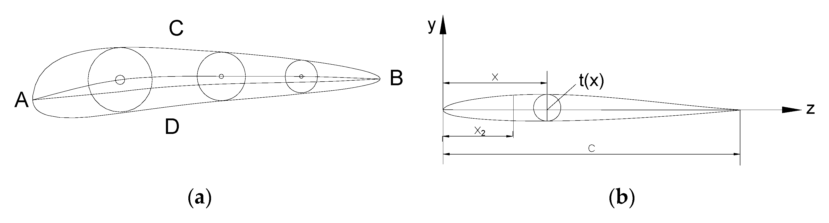
Chord: As shown in Figure 4a, the line between the frontmost point A of the airfoil and the rearmost point B of the airfoil is called the chord. The upper cambered surface of the chord is represented by $ABC$ in the figure, and the lower cambered surface is represented by $ABD$ in the figure. The value of the chord length $c$ is the length of the chord $AB$. It is the datum length of the airfoil.

(2)

Leading edge radius and leading edge angle: The leading edge refers to the frontmost point of the chord; the radius of the incircle at the leading edge of the airfoil is called the leading edge radius of the airfoil; and the angle between the tangent lines above and below the leading edge point is the leading edge angle.

(3)

Thickness and thickness distribution: As shown in Figure 4b, the X-axis passes through the chord, and the Y-axis passes through the frontmost end of the airfoil. The airfoil is divided into the upper and lower airfoils. The diameter of the tangential circle between the upper and lower airfoils is called the airfoil thickness represented by $t$ in the figure. The change rule of the thickness with $x$ is called thickness distribution and is expressed as $t\left(x\right)$.

The airfoil dynamic parameters of the airfoil mainly include the lift, the drag, the moment, the aerodynamic center (focus) and the center of pressure.

The hydrodynamic forces acting on the airfoil can be reduced to the lift and drag shown in Figure 5. The lift refers to the force in the direction perpendicular to the resultant velocity of water flow and is expressed as $F_L$; the drag is a force in the direction parallel to the resultant velocity of water flow and is expressed as $F_D$.

The lift coefficient $C_L$ and the drag coefficient $C_D$ are defined by the following relation formulas, respectively [8]:

$$C_L=\frac{L}{0.5\rho V_r^{2}c}$$

(13)

$$C_D=\frac{D}{0.5\rho V_r^{2}c}$$

(14)

where $L$ is the lift on the airfoil of the unit length, $N$; $D$ is the drag on the airfoil of the unit length, $N$; $c$ is the chord length of the airfoil, $m$; $V_r$ is the relative incoming velocity, $\mathrm{m}/\mathrm{s}$; and $\rho$ is the water flow solidity, $\mathrm{kg}/{\mathrm{m}}^3$.

The profile parameters of FX77-W-153 were optimized to improve its hydrodynamic performance. By comparing FX77-W-153 with NTS-XX20 in Figure 6 and Figure 7, it was found that although the CL of NTS-XX20 is greater than that of NTS-XX20, FX77-W-153 has a lower CD, which reduces the force on the blades, and the blade shape of FX77-W-153 was chosen after comprehensive consideration.

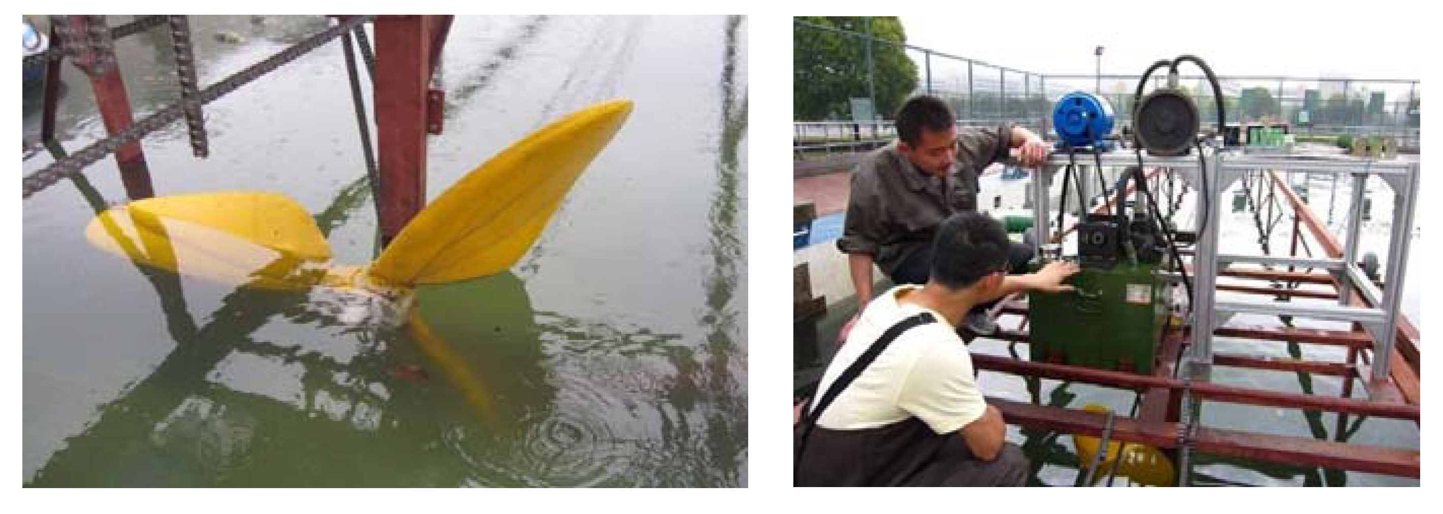
3. Design and Manufacture of the Tidal Current Energy Capture Device for the Experiment

Two blades were designed for this experiment. Blade I used the average flow rate of the seawater as the design flow velocity, Blade II used the maximum flow rate of the seawater. The main blade shape parameters were calculated using the MATLAB 2016 software programming optimization program. The 3D modeling of the blade was performed in combination with the Pro/E 5.0 software; the blade was processed by the numerical control (NC) center. Finally, the performance of the two blades was tested and compared on the experimental platform of the tidal current energy generation device [9].

3.1. Overall Design Parameters of Blades

The overall design parameters of the two blades are listed in

Table 2. The design parameters of two blades.

Parameter	Blade I	Blade II
Design flow velocity, $\mathrm{v}/\mathrm{m}{\mathrm{s}}^{-1}$	1.50	2.20
Number of blades, $B$	3	3
Blade diameter, $\mathrm{D}/\mathrm{m}$	1.30	1.30
Design speed, $\mathrm{n}/\mathrm{rpm}$	48	48
Hub diameter, $D_{hub}$/m	0.1	0.1
Tip speed ratio, $\lambda$	2.17	1.48
Blade airfoil	FX 77-W-153	FX 77-W-153

.

As can be seen from Table 2, the design flow velocity of the two blades was different. The number of blades is selected to be 3 due to the limitations of the test environment; the diameter of the blade is determined to be 1.3 m. The design speed of the blade is determined by the speed increaser ratio and generator speed. The speed is finalized to be 48 rpm after comprehensive consideration. The tip speed ratio of the two blades calculated by the tip speed ratio formulation λ is 2.17 and 1.48, respectively. The airfoil is FX77-W-153 [10].

3.2. Blade Design Steps

Based on the Wilson’s theory, the maximum energy utilization coefficient is considered to maximize the energy utilization coefficient for each blade element. The calculation steps for the blades are as follows:

(1)

After dividing the blades equally, the peripheral speed ratio of each section is calculated. The peripheral speed ratio ${\lambda }_i$ corresponding to the radius $r_i$ of the $i$th section is as follows [11]:

$${\lambda }_i={\lambda }_r\times \frac{r_i}{R}$$

(15)

(2)

The axial inducer $a_i$, the tangential inducer $b_i$ and the tip loss coefficient $F_i$ are calculated for each section $i$. This is also the process of solving the following conditional extreme value problem. The most important performance index of the blade is the energy capture coefficient$C_p$. In order to obtain the maximum capture coefficient, the $d{C}_p/d\lambda$ value of each blade element should be maximized. Therefore, the maximum value is taken as the objective function of optimization to obtain each parameter [12].

$$m\mathrm{in}:-d{C}_p=-\frac{8}{{\lambda }_0^2}b\left(1-a\right)F{\lambda }_0^{3}d\lambda$$

(16)

$$sub: \left(1-a_i{F}_i\right)=b_i\left(1+b_i\right){\lambda }_i$$

(17)

$$F=F_{tip}*F_{hub}$$

(18)

$$F_{tip}=\frac{2}{\pi }\left\{\exp \left[-\frac{\left(R-r\right)*B}{2R\sin \varphi }\right]\right\}$$

(19)

$$F_{hub}=\frac{2}{\pi }arccos\left\{\exp \left[-\frac{\left(r-R_{hub}\right)*B}{2R_{hub}\sin \varphi }\right]\right\}$$

(20)

The values $a,b$ can be solved by the nonlinearly constrained optimization function $FMINCON$ in the $MATLAB$ optimization toolbox.

(3)

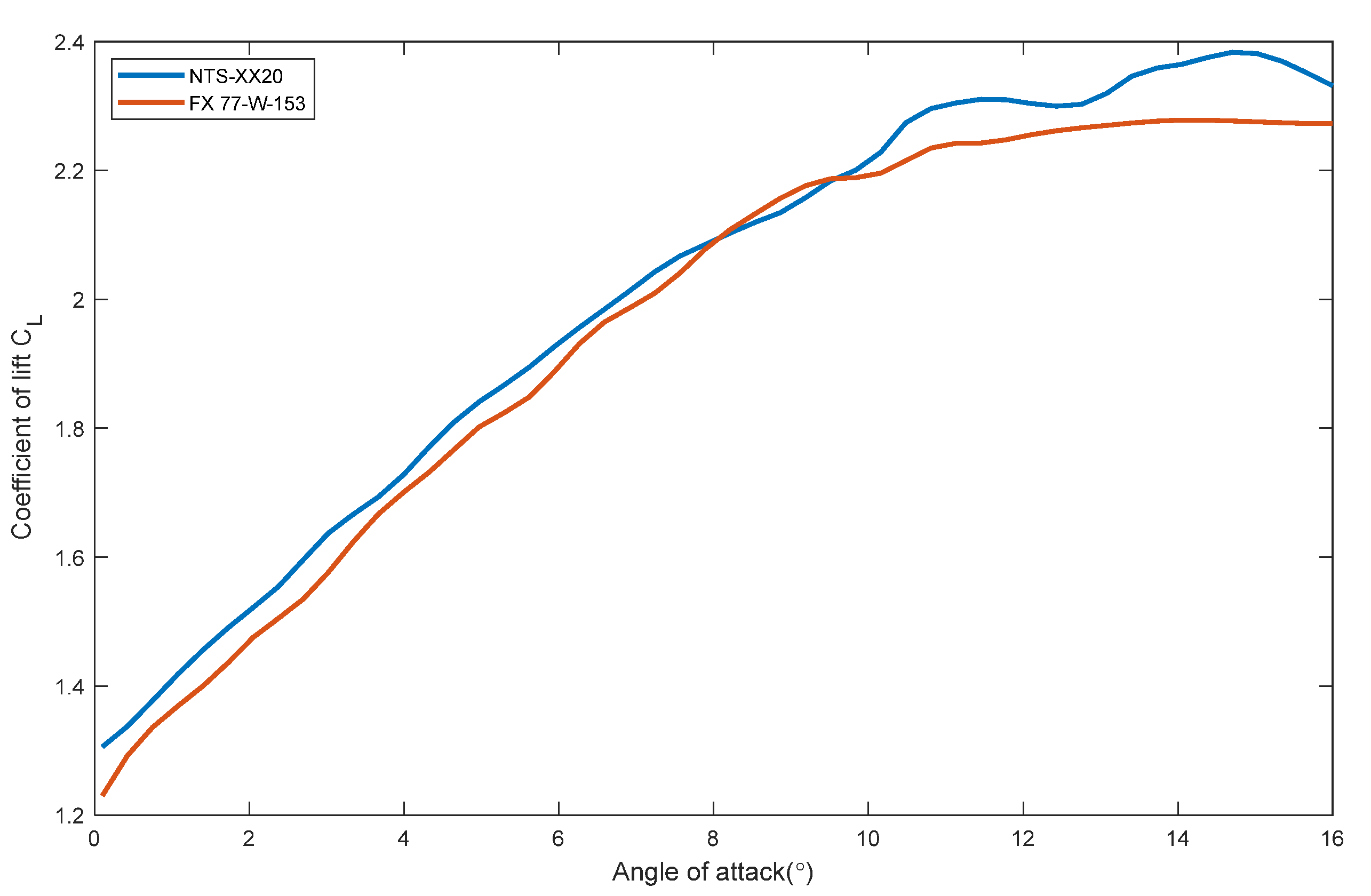
The airfoil type is selected using the Profili software. The curves of the optimum lift–drag ratio with the Reynolds number at different angles of attack can be calculated and analyzed by the software Profili 2.2. It can be calculated that the Reynolds number from the blade root to the blade tip is different. The lift coefficient $C_{Li}$ and drag coefficient $C_{Di}$ corresponding to these angles of attack can be determined by finding the angles of attack based on different lift–drag ratios according to the Reynolds number. However, since turbines have different powers, different radii and different distributions in each section, the angles of the attack required and the corresponding dynamic coefficient and drag coefficient also change greatly. For convenient design calculation, the relation between the angle of attack and lift coefficient of the airfoil can be determined using the $MATLAB$ software or a numerical calculation method [13] as follows:

$$C_L=f\left(a\right)$$

(21)

Similarly, the relation between the dynamic coefficient and drag coefficient of the airfoil can also be determined as follows.

$$C_D=g\left(C_L\right)$$

(22)

The installation angle ${\beta }_i$ is calculated. The dip angle ${\varphi }_i$ calculated by solving the conditional extrema is substituted into the formula

$${\beta }_i={\varphi }_i-a_i$$

(23)

to obtain the installation angle in each section.

The chord length $c_i$ is determined. The chord length

$$c_i=\frac{\left(1-a_i{F}_i\right)a_i{F}_i}{{\left(1-a_i\right)}^2}\times \frac{8\pi r_i}{B{C}_{Li}}\times \frac{{\sin }^2{\varphi }_i}{\cos {\varphi }_i}$$

(24)

The value $c_i$ can be obtained for each section by this formula.

During blade calculation, the chord length and a pitch angle of the corresponding blade element section can be obtained only by iteratively calculating the axial and tangential inducers of each blade section many times, which is costly and complicated. Therefore, blade parameters were calculated by the $MATLAB$ programming algorithm optimization in this paper [14].

Axial induction a and tangential induction b are obtained by quickly solving the nonlinear constraint equations with the function fmincon in the MATLAB optimization toolbox, and the chord length $c$ and pitch angle $\beta$ of the blade along the wingspan can be solved by substituting a and b into Equation (24).

The most important performance index of the blade design is the energy capture coefficient $CP$, and from Equation (16), the maximum capture coefficient is obtained by maximizing the value $d{C}_p/d\lambda$ for each lobe element. The function fmincon is used to solve for the minimum value of the function $-d{C}_p/d\lambda$ as the objective function, and the equilibrium Equation (17) is used as the constraint function for the calculation.

Table 3. Blade section parameters.

NO.	Position of Blade Element (m)	Axial Induction (a) of Blade I	Tangential Induction (b) of Blade I	Axial Induction (a) of Blade II	Tangential Induction (b) of Blade II	Thickness (%)
1	0.01	0.3356	1.0325	0.3221	2.6811	30
2	0.0437	0.3487	1.0468	0.2695	2.5475	28
3	0.0774	0.3210	0.6727	0.2806	1.2897	26
4	0.1111	0.3121	0.4813	0.2901	0.8085	24
5	0.1447	0.3109	0.3665	0.2979	0.5603	20
6	0.1784	0.3133	0.2905	0.3044	0.4125	20
7	0.2121	0.3171	0.2368	0.3101	0.3167	19
8	0.2458	0.3215	0.1972	0.3155	0.251	19
9	0.2795	0.3263	0.1671	0.3206	0.2041	19
10	0.3132	0.3314	0.1437	0.3259	0.1695	19
11	0.3468	0.3371	0.1254	0.3316	0.1434	18
12	0.3805	0.3435	0.1108	0.3379	0.1235	18
13	0.4142	0.3511	0.0993	0.3453	0.108	18
14	0.4479	0.3603	0.0902	0.3542	0.096	17
15	0.4816	0.3717	0.0831	0.3653	0.0868	17
16	0.5153	0.3800	0.0690	0.3797	0.08	17
17	0.5489	0.3800	0.0620	0.3809	0.0643	17
18	0.5826	0.3787	0.0471	0.3799	0.0571	16
19	0.6163	0.3708	0.0554	0.3688	0.0482	16
20	0.65	0.3303	0.0285	0.3572	0.0359	16

shows the axial inducer and tangential inducer in 20 sections of the two blades calculated using the MATLAB 2016 software. The eddy losses at the blade tip and root are considered, and the chord length and pitch angle are also modified by fitting.

Figure 8 and Figure 9 show the distribution curves of the chord length and pitch angle of the two blades, respectively. It can be intuitively seen from these figures that the average chord length of Blade I is greater than that of Blade II. Since the design speed of Blade II is high, and the design speed of the blade is inversely proportional to the solidity of the blade, the solidity of Blade I is higher. The distribution curves of the pitch angle of the blade show that the distribution curve of Blade I is slightly larger than that of Blade II.

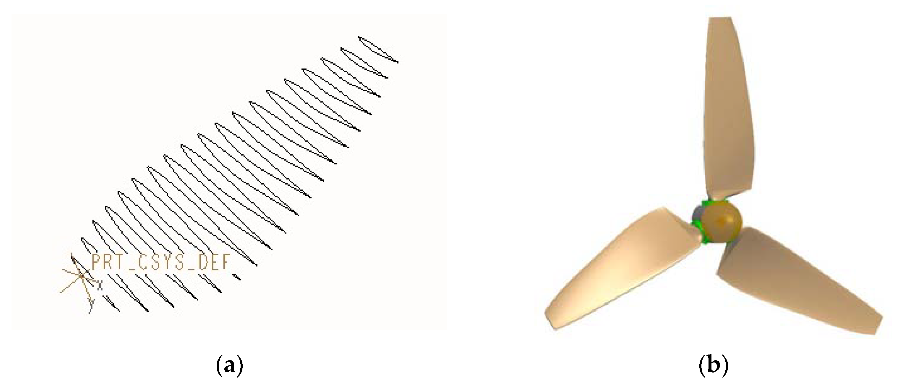
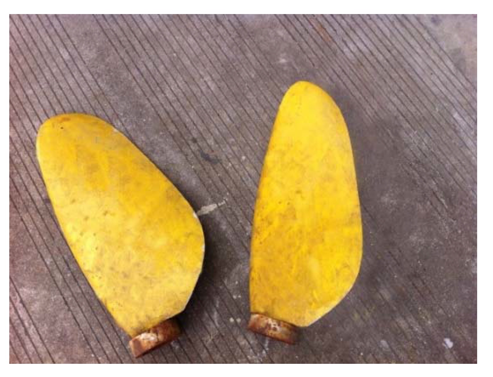
3.3. Processing and Production of Blade Model

In this study, after analyzing the lift–drag characteristics of multiple airfoils by the Profili 2.2 software, the FX 77-W-153 airfoil with excellent performance was selected. As shown in Figure 10,

Table 4. Some coordinates of the FX 77-W-153 airfoil.

X	Upper X	Lower Y
0	0	0
0.1082	0.5978	−0.46917
0.43291	1.381	−1.12723
0.97189	2.16847	−1.49776
1.72335	3.12598	−1.83573
2.68312	4.08078	−2.03599
3.84929	5.10965	−2.27645
5.21459	6.0881	−2.43568
6.77518	7.1001	−2.62006
8.52277	8.02742	−2.73455
10.44949	8.94786	−2.86996

lists partial 2D coordinate data of this airfoil. There usually are 100 pieces of data at a coordinate point of the airfoil. The maximum camber of this airfoil is 15.42%. At 28.2% of the airfoil, the maximum surface ratio is 4.53%. At 28.2% of the airfoil, the leading edge radius ratio of the chord is 1.5692%. The lift–drag curve is gentle. However, the lift–drag ratio is high, with the maximum lift–drag ratio at the attack angle of 12° [15].

According to the chord length and pitch angle in each section calculation in the previous section, the distribution curve of different pitch angles in the direction of the radius in the section of the blade section is complex in shape. The traditional method cannot meet the requirements for complex surface shape modeling. Therefore, in this paper, the MATLAB calculation tool was used to edit the space coordinate conversion function, convert the 2D coordinate points in each section blade element into the 3D coordinates of the actual position in space according to the requirements and then use the parametric modeling method of the Pro/E software to complete the 3D solid modeling of the blade.

3.4. Solid Modeling of Blade

The design results from the calculation by the blade design program are the space coordinates (x, y, z) of all discrete points in the 20 sections. The amount of data is very large. Therefore, the coordinate calculation function compiled by the MATLAB 2016 software can quickly and accurately calculate the coordinates of each point in batches and save it as a file required for the Pro/E parametric modeling to realize the parametric modeling of the blade element contour line.

The file of the blade element contour curve is imported through “Insert Datum Curve—From File” in the “Create Datum Curve” tool of Pro/E to transfer the design results to the Pro/E file and quickly generate the blade element contour line. Next, tools such as solid and surface modeling are used to draw the blades, hubs and other components. Finally, the blades are assembled. Figure 11a shows the blade element contour curve of Blade I. Figure 11b shows the 3D rendering of the assembled Blade I. The computational modeling method of Blade II is the same as above [16].

3.5. Material Selection and Processing of Blade

At present, the blade commonly used materials are aluminum, carbon fiber composite blade, glass fiber reinforced plastic blade and so on. Each material has its own range of applications and advantages and disadvantages. Attention should be paid to the following points:

(1)

Blades should be light, or they will increase the burden on other components such as hubs, controllers and generators, resulting in such defects as control delay and poor system coordination.

(2)

On the basis of blade design, the blade structure should be designed considering the influence of the actual operating environment factors of the unit, ensuring sufficient strength and stiffness of blades. This ensures that no damage occurs to blades in the provided service environment throughout their service life.

(3)

In terms of blade strength, static and fatigue strengths are usually analyzed and verified. The stability of pressurized parts should be verified to ensure that no deformation such as expansion, wrinkling and warping occurs in materials. The strength analysis is mainly based on the loads on blades. Inertial loads, gravity, motion loads and other loads are mainly calculated.

In summary, the blade for this experiment is made of FRP material, and the NC module in the Pro/E software is used to automatically compile the NC code for blade mold processing and import the NC center to process the blade wood mold. Figure 12 shows the physical comparison of the two types of blades processed.

4. Analysis of Blade Test Data

The two blades designed were distributed and installed on the platform for performance testing. At different flow velocities, the blade speed, capture power of blades, the thrust thereon and other data are collected and analyzed to comprehensively test and compare the performance of the blades. Figure 13 shows the experimental site for the performance test of the two blades.

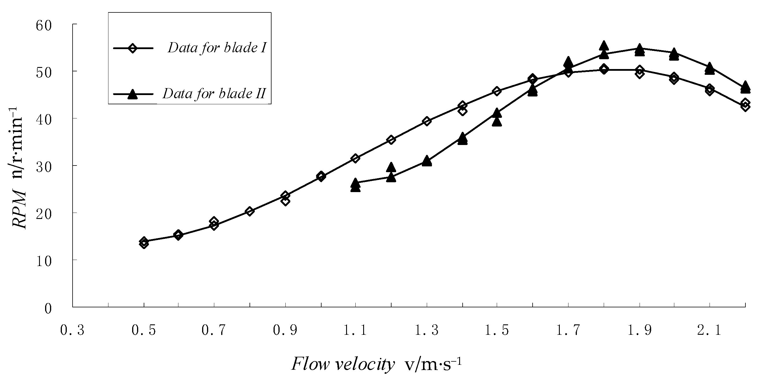
4.1. Start Flow Velocity Comparison Experiment

The purpose of the experiment is to study the starting flow velocity of the two blades and test their self-starting performance. Figure 14 shows the speed distribution of the two blades at different flow velocities. It can be seen that the starting flow velocity of Blade I is 0.5 $\mathrm{m}/\mathrm{s}$. As the flow velocity increases, the blades speed up, causing the generator input speed to speed up too. In order to ensure that the generator works at the best efficiency point, its speed should be controlled near the rated speed. Therefore, the test system automatically matches the loads, controls the speed of the blades and stabilizes the output power. The start flow velocity of Blade II is relatively high, 1$\mathrm{m}/\mathrm{s}$. Since its design speed is high, solidity is low, the lift obtained is relatively small, but its speed after starting is higher than that of Blade I. In order to stabilize the output power, the speed is limited. Figure 15 shows the tip speed ratio distribution curves of the two blades calculated by collecting data. It can be intuitively seen that the tip speed ratio of Blade I is higher than that of Blade II, when the flow velocity is 0.5~1.7. Since the capture efficiency of blades is a function of the tip speed ratio and pitch angle, it can be known by substituting the pitch angle and tip speed ratio in the experiment described in this flow velocity section. The capture efficiency of Blade I is higher than that of Blade II. In summary, the starting performance of Blade I is better than that of Blade II in this flow velocity range. Blade I can start to capture energy at low flow velocity; its energy capture efficiency is relatively high.

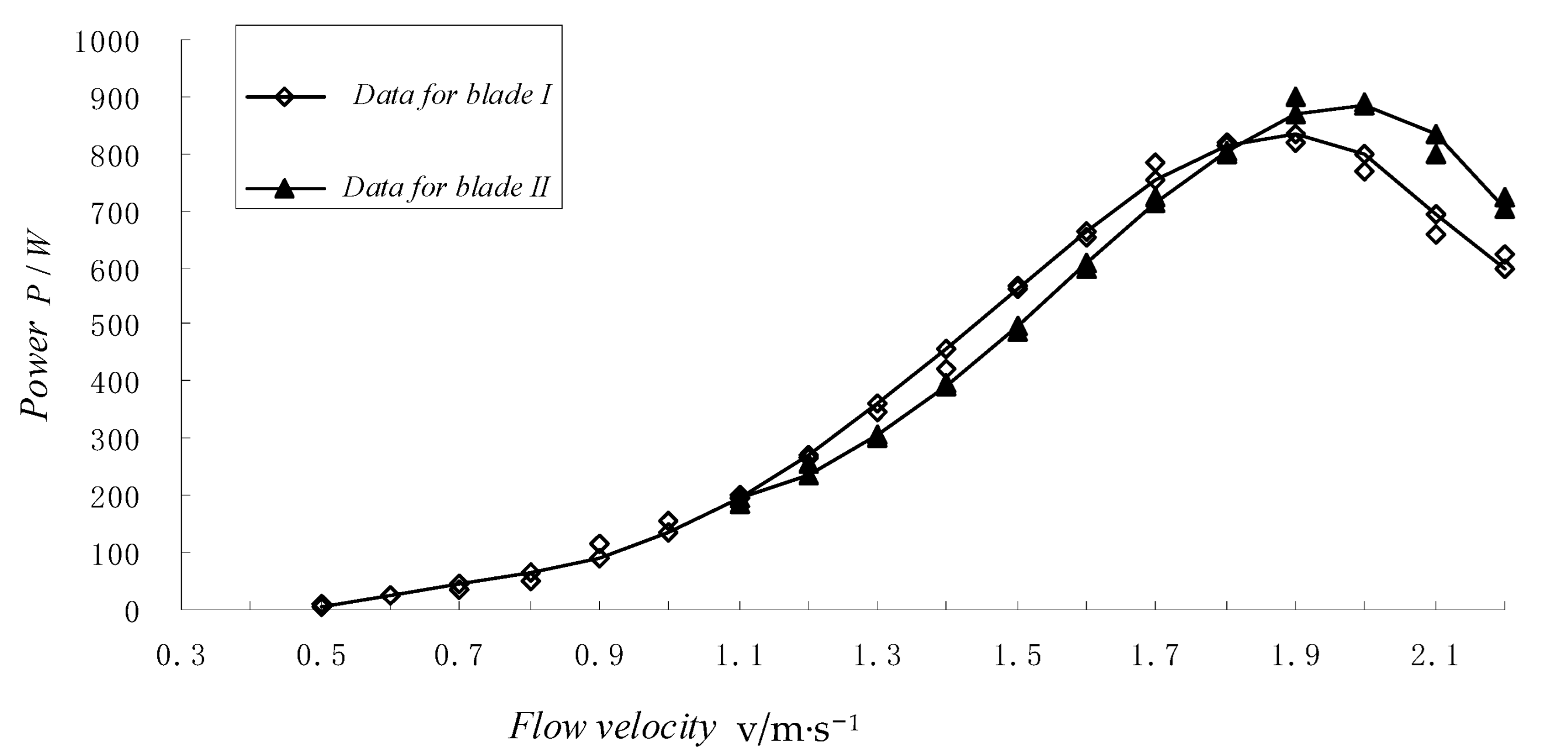
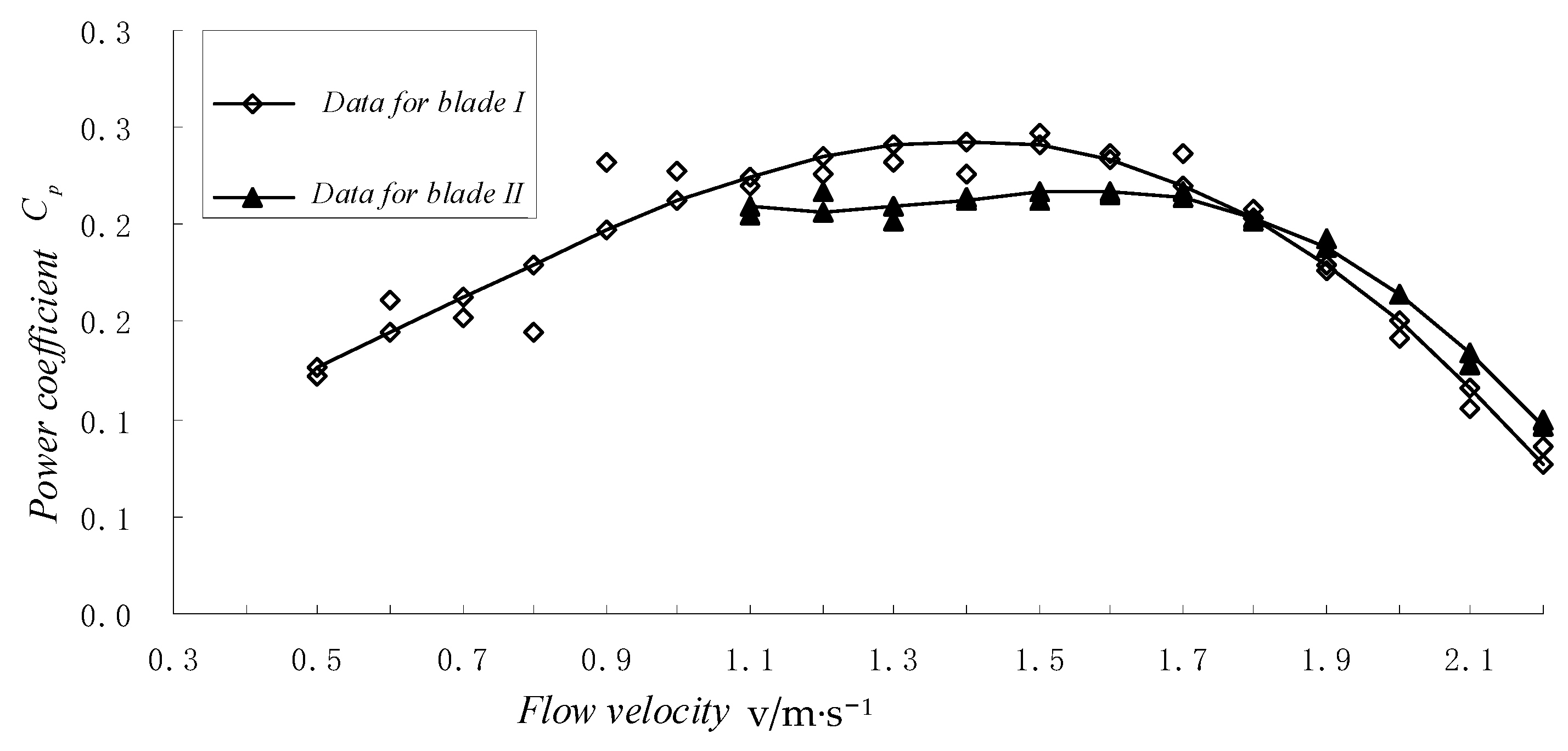
4.2. Generation Power Comparison Experiment

The purpose of the experiment is to investigate how much total power is generated by the two blades and determine the power coefficient under the changing flow velocities. Figure 16 shows the distribution of the experimental data of the power generated by the two blades at different flow rates. It can be seen that before the flow velocity of 1.9 $\mathrm{m}/\mathrm{s}$, the generation power of Blade I is greater than that of Blade II. When the flow velocity is above 2 $\mathrm{m}/\mathrm{s}$, the generation power of Blade II is greater than that of Blade I. The reason for this is that the design flow velocity of Blade II is 2.2 $\mathrm{m}/\mathrm{s}$. When the tidal flow velocity approaches its design flow velocity, although the capture efficiency is high, according to the characteristics of the tidal flow velocity, the period in which the tidal flow velocity is higher than 2 $\mathrm{m}/\mathrm{s}$ in a day is very short. Therefore, the performance of Blade I is better than that of Blade II most of the time. In a tide cycle, although Blade I fails to output the highest power at the same moment as Blade II, Blade I has the highest capture efficiency.

Figure 17 shows the graph of the flow rate power coefficient. The maximum power coefficient of Blade I appears near the design point, which verifies the validity of the design calculation method proposed in this paper. The optimum tip speed ratio is not reached because of the limitations imposed by the diameter and speed of the blades. Therefore, the highest point power factor is 0.23.

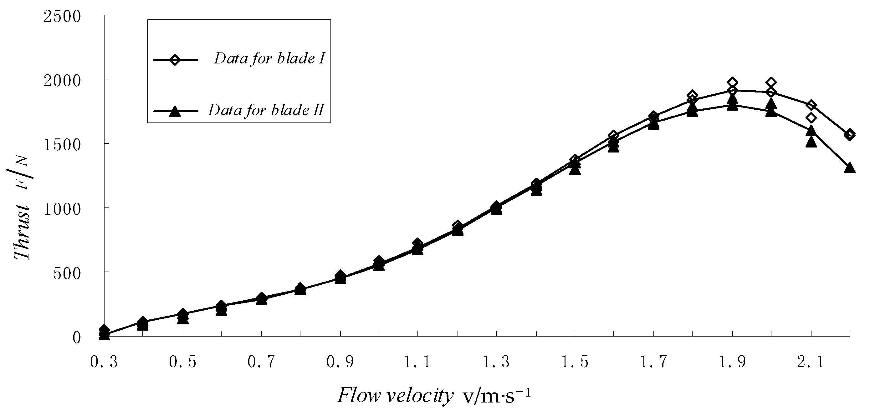
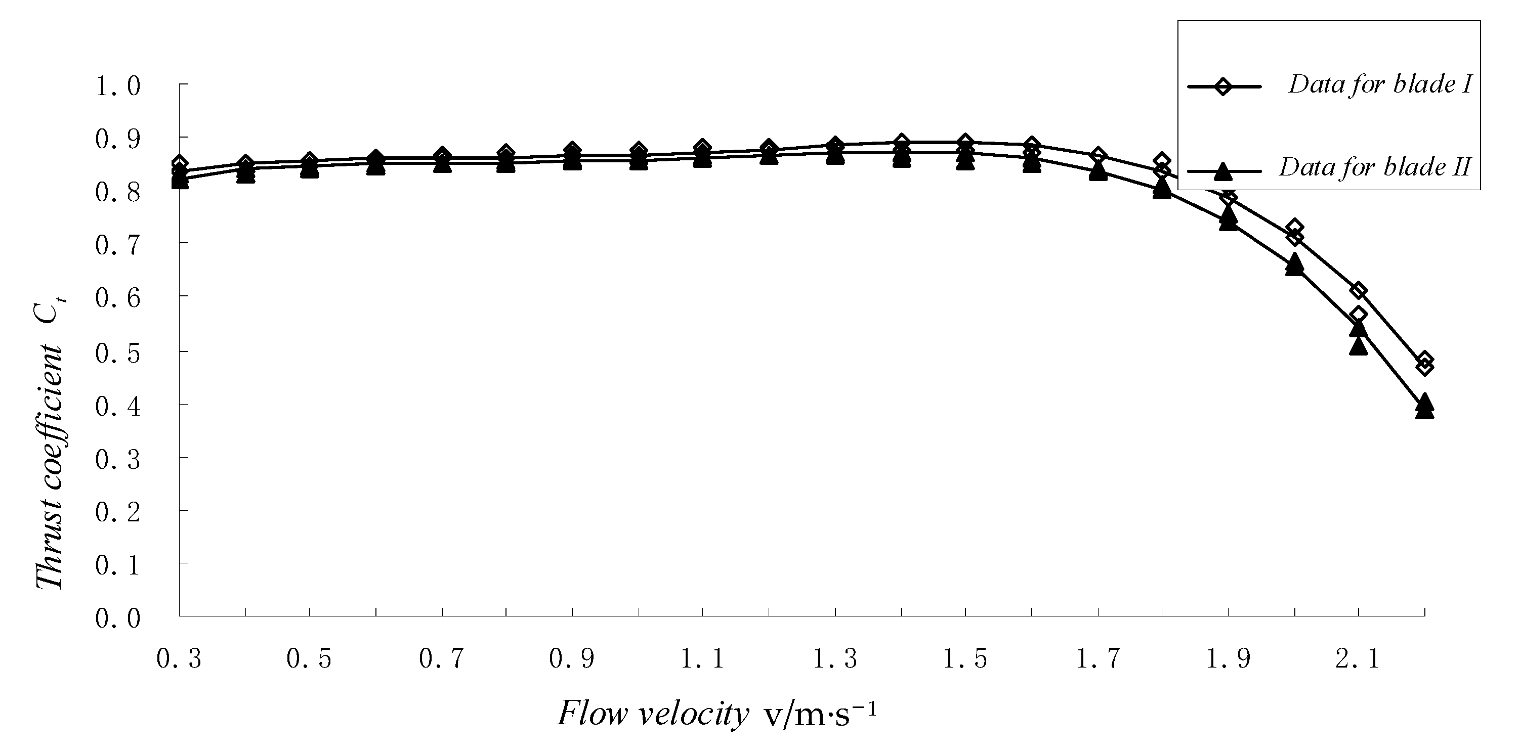
4.3. Blade Thrust Experiment

Figure 18 shows the thrust distribution curve of the two blades at changing flow velocities. It can be seen from the figure that in the range of flow velocity of 0.3~1.5 m/s, the thrust of Blade I is greater than that of Blade II. When the flow velocity is above 1.5 m/s, the thrust of Blade I increases greatly relative to Blade II. Since the solidity of Blade I is higher than that of Blade II, and the thrust is proportional to the square of the flow velocity, the thrust thereon will inevitably be great. At a flow velocity of about 2.0 $\mathrm{m}/\mathrm{s}$, the thrust on Blade I reaches the maximum value, which is close to 2000 N. Therefore, this is also the allowable thrust for the design strength for the blades and the mounting frame.

Figure 19 shows the variation curves of the thrust coefficient of the two blades. Before the flow velocity reaches 1.7 m/s, the thrust coefficient of the two blades is basically around 0.8. When the flow velocity is above 1.7 m/s, the thrust coefficient of the two blades decreases. Since the blade speed is limited to the scope allowed by the generator, as the flow velocity increases, the control system ensures that the blade speed basically remains unchanged by load matching. The thrust coefficient decreases accordingly.

5. Experimental Conclusions

By analyzing and comparing the experimental data from the above blade performance tests, the following conclusions were drawn.

1.

The design flow velocity has a great impact on the solidity of turbine. When the pitch angle is unchanged, increasing the blade solidity can effectively improve the self-starting performance of the blade. Nevertheless, since the blade speed and solidity are inversely proportional, the two should be taken into consideration when selecting the appropriate design flow velocity.

2.

A comparison of power generation experiments shows that at low flow rates, Blade I generates more power than Blade II, and as the flow velocity increases, Blade II generates more power than Blade I. Therefore, choosing the appropriate blade allows the turbine to capture the most power over a varying range of flow rates.

3.

The test comparison in the thrust experiment showed that throughout the range of flow velocity, the thrust on Blade I is greater than that on Blade II. This is also due to the high blade solidity and is inevitable.

In this paper two blades of different solidity have been designed and manufactured: The varying design flow velocity has a great influence on the solidity of the blades. In addition, the two blades were machined. The experimental data were analyzed and compared in a blade test platform experiment, which proved the correctness and applicability of the blade design and calculation method proposed here.

References

1. Colby, J.A.; Corren, D.R.; Pe, M.A.A.; Hernandez, A.A. Advancement of a Tidal Energy Converter Mount Through Integrated Design Process and Risk Management. In Proceedings of the Offshore Technology Conference, Houston, TX, USA, 6–9 May 2019. [Google Scholar]
2. Ma, S.; Li, W.; Liu, H.; Lin, Y. Research on the Energy Capture Device of Horizontal Axis Tidal Current Energy Conversion Systems. J. Mech. Eng. 2010, 46, 150–156. [Google Scholar] [CrossRef]
3. Li, G.; Zhu, W. A Review on Up-to-Date Gearbox Technologies and Maintenance of Tidal Current Energy Converters. Energies 2022, 15, 9236. [Google Scholar] [CrossRef]
4. Seo, J.; Yi, J.H.; Park, J.S.; Lee, K.S. Review of tidal characteristics of Uldolmok Strait and optimal design of blade shape for horizontal axis tidal current turbines. Renew. Sustain. Energy Rev. 2019, 113, 109273. [Google Scholar] [CrossRef]
5. Goundar, J.N.; Ahmed, M.R. Design of a horizontal axis tidal current turbine. Appl. Energy 2013, 111, 161–174. [Google Scholar] [CrossRef]
6. Mahmuddin, F. Rotor blade performance analysis with blade element momentum theory. Energy Procedia 2017, 105, 1123–1129. [Google Scholar] [CrossRef]
7. Li, Y.; Liu, H.; Lin, Y.; Li, W.; Gu, Y. Design and test of a 600-kW horizontal-axis tidal current turbine. Energy 2019, 182, 177–186. [Google Scholar] [CrossRef]
8. Borg, M.G.; Xiao, Q.; Allsop, S.; Incecik, A.; Peyrard, C. A numerical performance analysis of a ducted, high-solidity tidal turbine. Renew. Energy 2020, 159, 663–682. [Google Scholar] [CrossRef]
9. Sagharichi, A.; Zamani, M.; Ghasemi, A. Effect of solidity on the performance of variable-pitch vertical axis wind turbine. Energy 2018, 161, 753–775. [Google Scholar] [CrossRef]
10. Faizan, M.; Badshah, S.; Badshah, M.; Haider, B.A. Performance and wake analysis of horizontal axis tidal current turbine using Improved Delayed Detached Eddy Simulation. Renew. Energy 2022, 184, 740–752. [Google Scholar] [CrossRef]
11. Wang, S.; Zhang, Y.; Xie, Y.; Xu, G.; Liu, K.; Zheng, Y. The effects of surge motion on hydrodynamics characteristics of horizontal-axis tidal current turbine under free surface condition. Renew. Energy 2021, 170, 773–784. [Google Scholar] [CrossRef]
12. Kim, S.J.; Singh, P.M.; Hyun, B.S.; Lee, Y.H.; Choi, Y.D. A study on the floating bridge type horizontal axis tidal current turbine for energy independent islands in Korea. Renew. Energy 2017, 112, 35–43. [Google Scholar] [CrossRef]
13. Wang, S.; Zhang, Y.; Xie, Y.; Xu, G.; Liu, K.; Zheng, Y. Hydrodynamic analysis of horizontal axis tidal current turbine under the wave-current condition. J. Mar. Sci. Eng. 2020, 8, 562. [Google Scholar] [CrossRef]
14. Ledoux, J.; Riffo, S.; Salomon, J. Analysis of the blade element momentum theory. SIAM J. Appl. Math. 2021, 81, 2596–2621. [Google Scholar] [CrossRef]
15. Dehouck, V.; Lateb, M.; Sacheau, J.; Fellouah, H. Application of the blade element momentum theory to design horizontal axis wind turbine blades. J. Sol. Energy Eng. 2018, 140, 014501. [Google Scholar] [CrossRef]
16. Borg, M.G.; Xiao, Q.; Allsop, S.; Incecik, A.; Peyrard, C. A numerical structural analysis of ducted, high-solidity, fibre-composite tidal turbine rotor configurations in real flow conditions. Ocean Eng. 2021, 233, 109087. [Google Scholar] [CrossRef]
Figure 1. (a) Water Turbine of Verdant Power, USA [1]; (b)Water Turbine Device of Zhejiang University [2].
Energies 16 03467 g001
Figure 2. (a) Water turbine with high solidity [3]. (b) Water turbine with low solidity [3].
Energies 16 03467 g002
Figure 3. Force analysis of the blade.
Energies 16 03467 g003
Figure 4. (a) The chord of airfoil. (b) The thickness of the airfoil.
Energies 16 03467 g004
Figure 5. The forces of the airfoil.
Energies 16 03467 g005
Figure 6. Variation of the coefficient of lift for NTS-XX20 compared with that of FX 77-W-153 at different AOA and Re = 2 × 10⁶.
Energies 16 03467 g006
Figure 7. Variation of the coefficient of drag for NTS-XX20 compared with that of FX77-W-153 at different AOA and Re = 2 × 10⁶.
Energies 16 03467 g007
Figure 8. The chord length and pitch angle of Blade I.
Energies 16 03467 g008
Figure 9. The chord length and a pitch angle of the Blade II.
Energies 16 03467 g009
Figure 10. The two-dimensional diagram of airfoil.
Energies 16 03467 g010
Figure 11. (a) Blade element diagram of Blade I. (b) Three-dimentional modeling diagram of Blade I.
Energies 16 03467 g011
Figure 12. Comparison of two blades with different solidity.
Energies 16 03467 g012
Figure 13. Blade performance test experiment.
Energies 16 03467 g013
Figure 14. RPM of the blade at different velocities.
Energies 16 03467 g014
Figure 15. Tip speed ratio of the blade at different velocities.
Energies 16 03467 g015
Figure 16. Power of the blade at different velocities.
Energies 16 03467 g016
Figure 17. Power coefficient of the blade at different velocities.
Energies 16 03467 g017
Figure 18. Thrust of the blade at different velocities.
Energies 16 03467 g018
Figure 19. Thrust coefficient of blades at different flow velocities.
Energies 16 03467 g019