1. Introduction
The rational use of water and energy, which are vital natural resources, is the cornerstone of sustainable development. The interdependencies between water and energy are well known. Under the term of water and energy nexus (WEN) they have been of interest to scientists for many years [
1,
2,
3]. It is estimated that the production and transport of water consumes about 7% of global electricity consumption, of which more than 90% is related to pumping [
3,
4]. Therefore, also increasing energy efficiency in the water supply sector is one of the economic policy priorities of countries around the world. An example of this can be found in, e.g., the EU Directive on energy efficiency [
5], which assumes an increase in energy efficiency by 20% by 2020 and by, at least, 32.5% by 2030 [
6].
In addition to the obvious ecological dimension related to the reduction in raw material consumption or the reduction in greenhouse gas emissions, the increase in the energy efficiency of the water distribution network (WDN) has an equally important economic aspect; this is because the cost of electricity is the second largest component (after personnel costs) of water supply companies’ operating costs. Improving the energy efficiency of WDNs can be the result of simple actions in the form of both controlling and reducing water leaks, as well as by utilizing more complex tools including, e.g., the prediction of water demand, the optimization of the operation of pump units and water tanks, real-time control of system elements, etc., which would be conducted while maintaining all required technical parameters of the system at any time, and by taking into account the needs of all users. For this reason, it becomes necessary to use computer modeling and to utilize dynamic simulations of WDN operations [
7].
During the system’s energy audit, a number of metrics are used to evaluate the energy efficiency. The methodology of conducting energy audits has been discussed many times in the literature [
7,
8]. This is because doing so provides the opportunity to choose the method and energy indicators that are best suited to a specific case, taking into account the specificity of the system, the availability of data and analytical tools, and, finally, the purpose of the analysis. The audit procedure should be carefully thought out, prepared, and may include the following activities [
9]: the creation of an assessment team, recognition of the tested system, data collection, energy balance, a selection of energy indicators, a preliminary analysis of results, arrangements with the contracting authority, a final report, etc. The key elements among the abovementioned activities are the energy balance taking into account the various forms of energy supplied to the system, its transformations, and the energy supplied to users, as well as numerical indicators allowing for a measurable and objective assessment of the system under study.
Cabrera et al. [
10] proposed the following components of the WDN energy balance: external energy supplied by water intakes/reservoirs/tanks (
EN), energy supplied by pump drives (
EP), energy delivered with water to consumers (
EU), outgoing energy due to leaks/water loss (
EL), energy loss in pipes due to friction (
EF), and energy compensation in network tanks (
EC), with the aim of the
EC being zero when the long term balance is considered. The above components of energy balance were used to determine the energy efficiency indicators, characterizing such system properties as excess energy supplied, the energy efficiency of WDN, the relative energy loss due to friction, as well as the relative energy loss due to leakage or the meeting of the required standard of water supply in terms of service pressure.
A similar component of the energy balance was identified in a study by Mamade et al. [
11,
12], who proposed, for the purposes of an assessment of energy efficiency, an indicator of total energy excess in relation to the minimum energy demand. The comparison of two methods of energy balancing was also provided: simplified (top-down) method, based on the use of cumulative data on water consumption and losses, as well as the required pressure in the network, which does not require a hydrodynamic modeling of the WDN; and a complex (bottom-up) method, based on a calibrated hydraulic model of the WDN, which allows for the analysis of energy consumption by each element of the system.
Due to the fact that the possibilities of reducing the energy loss due to friction in water pipes (
EF) or reducing the available pressure at consumers (
EU) are limited in the existing WDN—in addition to the abovementioned components of energy balance—the optimization of energy consumption associated with water pumping (
EP), as well as the minimizing of losses (leaks) of water and related energy “escaping” from the system (
EL), can have the greatest impact on improving the energy efficiency of the WDN. The first of these problems, as a rule, requires the determination of the optimal pump operation schedule. This is achieved by taking into account the hydraulic characteristics of the pumps, the volume of water storage tanks, and the variability of electricity prices (including night tariffs). Various techniques are used to solve such multi-objective optimization tasks, ranging from the simplest methods of linear programming to advanced heuristic methods in combination with the results of the hydraulic modeling of the WDN [
13,
14,
15,
16]. Reducing water losses is one of the greatest challenges of water supply companies and requires coordinated actions related to both the location of water leaks, the determination of the amount of “leaking” water, as well as the method of controlling and reducing water losses in the system [
17]. Additionally, in this case, the results of hydraulic modeling of the network are commonly used [
18,
19].
It is also worth mentioning one of the most widely used systems for comprehensively assessing the functioning of water supply systems, which is developed by the International Water Association (IWA) [
20]. Energy indicators are one of the elements of this methodology and include such physical and economic parameters as percentage use of pump capacity, standardized electricity consumption, electricity recovery, reactive electricity consumption, and electricity cost.
While the above information indicates that the methodology of energy audits is well recognized, the practical assessment of the energy efficiency of the WDN may be difficult. This can be especially true for extensive and diverse systems in which district metering areas (DMA) have not yet been developed, and thus the availability of operational data may be limited, and the quantitative verification of water leaks is difficult. By analyzing the available sources, it can be also seen that many previous works were based on either specially prepared benchmark models [
10,
19] or on the simplified, real models of small and medium-sized WDNs [
12,
21]. Wide area networks, which are, additionally, often oversized, have been analyzed less frequently [
22,
23].
One of the most difficult problems to solve is modeling the energy losses associated with water leakage. It is possible to use both simplified iterative methods (successive approximations) [
11,
19] and heuristic-stochastic methods, including genetic algorithms, Monte Carlo simulations [
24], and artificial neural networks [
25]. The other approach is presented by Berardi et al. [
26] who proposed distributing water losses consistently with the deterioration processes of pipelines with the key role of mass balance in enhanced hydraulic models.
When looking at the practical aspect, each time it is a difficult process, requiring either time-consuming calculations or specialized software and trained analysts. Therefore, in this paper, we propose a novel method based on a simplified water balance in the system and the use of the index of unavoidable average real loss (
UARL) developed by the IWA [
27]. This method allows one to take into account the different quantitative characteristics of leakages for feeder and distribution mains and service connections, and additionally significantly simplifies the procedure of calibrating the water leakage model in the network. This method, applied to the examined WDN, made it possible to determine the energy indicators of the system under study and to indicate those system elements that should be first analyzed by the water supply company in terms of optimizing energy efficiency.
This paper is organized as follows:
Section 2 provides the methodological background for the research carried out, including a description of the WDN that is the subject of the case study (
Section 2.1); an explanation of the energy audit procedure proposed by Cabrera et al. [
10] (
Section 2.2); as well as the development of the innovative method of linking water losses model that was proposed by IWA with the hydrodynamic modeling environment, e.g., Epanet (
Section 2.3).
Section 3 presents the results of the energy audit of the tested water supply network. Then,
Section 4 discusses and interprets the most important indicators of the system’s energy efficiency. The article ends with
Section 5, which contains a summary of the conducted research and indications of directions for further work in order to verify and improve the proposed method of modeling water losses in WDNs.
2. Materials and Methods
Due to the relatively complex structure of the studied WDN (which is described in detail in
Section 2.1), the “bottom-up” approach was used in the presented research, using the hydrodynamic model of the network developed in Epanet 2.2 software [
28]. The calibrated model was used to simulate the operation of the network during an average demand for water, with a time step of 10 min for the hydraulic calculations and a reporting of the results every 1 h. The simulation results were used to prepare a global energy balance, according to the model proposed by Cabrera et al. [
10], and is shown in
Figure 1. The mathematical basis and the method of determining the energy indicators for the tested system are described in
Section 2.2. The water leaks play an important role in the assessment of the energy efficiency of the WDN; therefore,
Section 2.3 describes, in detail, the methodology for calibrating the emitters’ coefficients for simulating water leakage in network nodes.
2.1. Characteristics of the WDN under Study
The studied water supply network serves the town of Polanica-Zdrój, located in south-western Poland. The WDN is characterized by a very extensive structure, which consists of 2 main groundwater intakes (BS1, BS4/6 drilled wells) cooperating with the ZSS water storage tank with a capacity of 744 m3; auxiliary intakes PIA (drainage) and a POL (dug well) cooperating with the ZP tank with a capacity of 880 m3; the ZD water storage tank with a capacity of 690 m3, which is supplied directly from the feeder main; as well as reserve intakes UJ (surface water) and UWP (underground), which are currently not in use for technical reasons. The BS4/6 wells also feed the ZR tank, which has a capacity of 40 m3. A small part of the network is supported by the HZ buster pumping station, which cooperates with the ZNS storage tank that has a capacity of 26 m3, which can also be filled from the UJ intake (when active). The cooperation of water sources with storage tanks is based on a typical pump control system that depends on the level of water in tanks. Only pumps in the BS4/6 wells can also be time controlled.
Due to the significant denivelation of the service area (the difference in levels between the main reservoir supplying water to the network-ZSS and the lowest located node of the network is over 120 m), there are 19 pressure reducing valves (PRVs) in the network, which divide the supply area into several zones of regulated pressure.
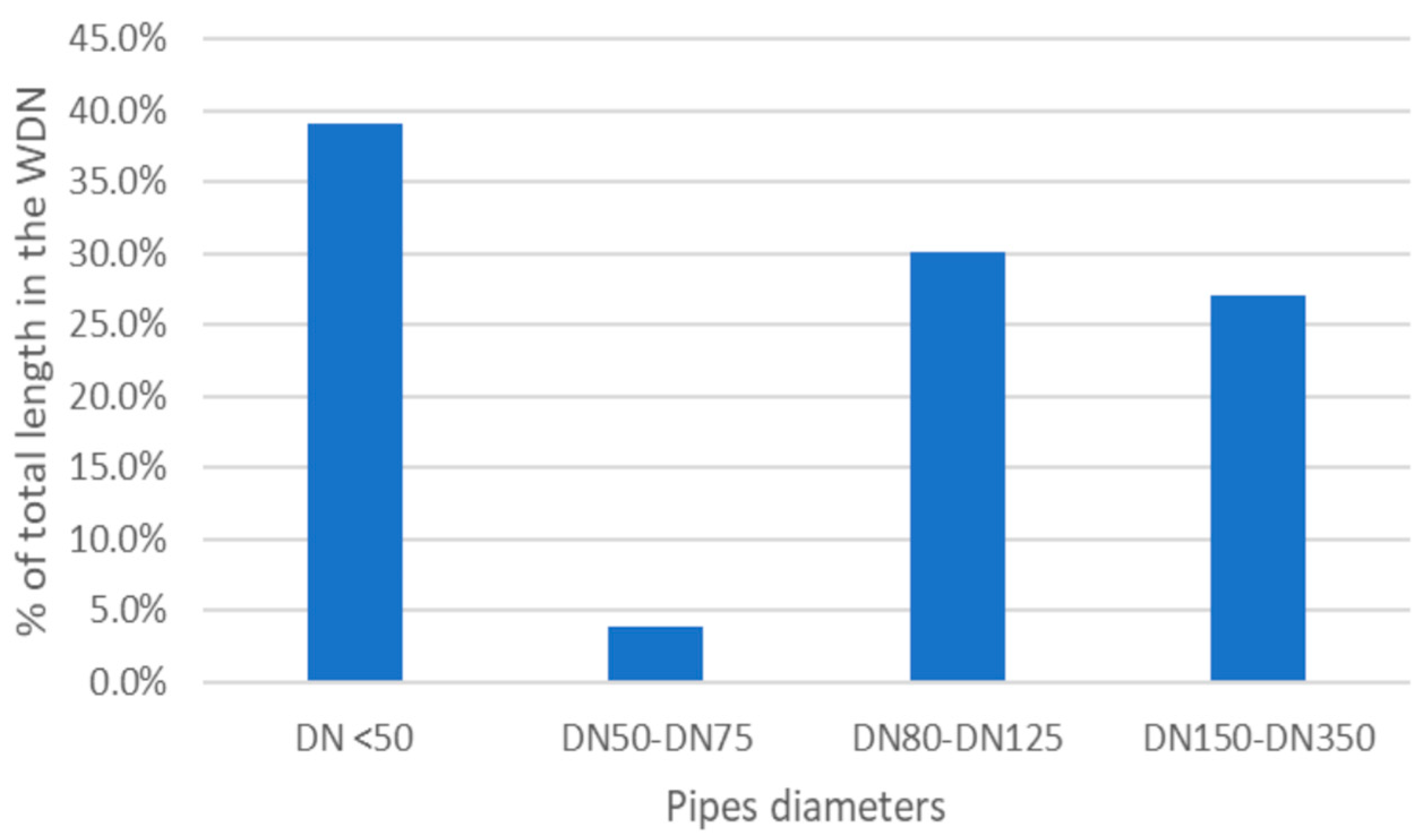
The water supply network has a total length of 101.6 km, of which 57.2% are feeder and distribution mains, and 42.8% are service connections. The total length of the mains is
LM = 58.10 km, and the service connections’
LSC = 43.50 km. The diagram of the WDN is presented in
Figure 2, and the structure of the diameters in the network is shown in
Figure 3.
The network model was built in the Epanet program based on the data contained in the GIS database. The model consists of 4198 sections and 4148 nodes, of which 952 are nodes supplying water to consumers. The model was calibrated based on data from several measurement campaigns carried out in different periods of 2021, during which water consumption by various groups of consumers and pressure in selected zones of the city were monitored.
2.2. Energy Efficiency
The energy balance of the WDN presented in
Figure 1 can be expressed for a specific simulation time
tp using Equation (1) [
10]:
where
Einput(
tp)—energy supplied to the system;
EN(
tp)—input energy supplied by the water sources;
EP(
tp)—energy supplied by the pumps (shaft work);
EU(
tp)—energy delivered to the water consumers;
EL(
tp)—energy discharged with water leaks;
EF(
tp)—friction energy; Δ
EC(
tp)—energy compensation in water storage tanks;
Eoutput(
tp)—energy discharged (to consumers and via water leaks); and
Edissipated(
tp)—energy dissipated (due to friction).
Individual forms of energy are calculated from the following relationships:
- (a)
Input energy supplied by the water sources:
where
VNi—volume of water supplied from the
i-th reservoir in the period
tp;
HNi—piezometric height of water in the
i-th reservoir;
nN—the number of water sources; and
γ—specific weight of water.
- (b)
Energy: pumping, delivered to customers, energy lost from water leaks, and friction energy (X = P, U, L, F):
for X = P (pumping), nP—number of pumps in the system; QPi(tk)—efficiency of the i-th pump in time tk; and HPi(tk)—head of pump i in time tk;
for X = U (users), nU—number of nodesbelonging to service connections; QUi(tk)—flow rate in the i-th node of the connection point in time tk; and HUi—piezometric head in the i-th junction node at time tk;
for X = L (leakage), nL—number of network nodes; QLi(tk)—water loss in the i-th node in time tk; and HLi(tk)—pressure head in the i-th node at time tk;
for X = F (friction), nF—number of network sections; QFi(tk)—water flow on the i-th section (taking into account water losses) in time tk; and HFi(tk)—pressure loss on the i-th section in time tk;
Δt—length of the time interval for the simulation (tk+1 − tk).
- (c)
compensation of energy in the water storage tank:
where
nC—number of storage tanks;
Ai—water surface in the
i-th storage tank;
Zi(
tp)—filling of the
i-th tank at the end of the simulation period; and
Zi(
t1)—filling of the
i-th tank at the beginning of the simulation period.
The above relationships are used to calculate the energy indicators listed below [
10]:
- (d)
excess energy supplied to the system:
- (e)
WDN energy efficiency:
- (f)
friction energy loss:
- (g)
leakage energy loss:
- (h)
standard compliance:
The parameter
EUmin(
tp) is present in Equations (5) and (9); it determines the minimum required energy delivered to water consumers, which is calculated as follows:
where
HMINi(
tk)—minimum piezometric head required in the
i-th node of the service connection.
In turn, the parameter
EF′(
tp) determines energy loss due to friction in an “ideal” network, i.e., without water leaks, which can be obtained from the Equation (11):
where
QFi′(
tk)—water flow on the
i-th section (without leaks) in time
tk; and
HFi′(
tk)—pressure loss on the
i-th section in time
tk at the flow
QFi′(
tk) (no leaks).
It is also important to remember that each system is different in terms of energy input. There are systems that need significant amounts of energy to pump water (
EP), others may be characterized by a large share of natural energy (
EN), e.g., from water sources located above the service area. Therefore, relative natural energy input (
RN) or relative pump energy input (
RP), which are estimated as the portion of energy input that is natural or supplied by pumps (Equation (12)), should also be taken into account when comparing the energy efficiency of different systems or different operational scenarios for a given WDN.
2.3. Water Leaks
To model water leaks using the Epanet, the emitter flow rate in a network node is used, as determined from the Equation (13) [
28]:
where
CE—emitter discharge coefficient,
p—water pressure in the node, and
N—exponential coefficient depending on the type of emitter; furthermore, in the case of modeling water leaks, it is often assumed that
N is in the range of 0.5–2.0, depending on the pipe material [
27]. Parameters
C and
N can be estimated based, for example, on the analysis of night water flows [
29] or on the basis of mass balance and hydraulic modeling results [
19].
The authors of the energy audit methodology described in
Section 2.2 suggest an iterative method for modeling leaks based on the mass balance of water in the system, assuming that the size of the leak in a node is proportional to the water pressure and the length of sections connected in a given node (weighted node length) [
19]. This method, however, seems to be relatively laborious, due to the need to assign a factor of weighted nodal length to each node. Due to the structure of the model used in this study (consisting of over 4000 nodes), the use of this method would require a significant amount of work. Therefore, we developed a simplified calibration method based on the mass balance and water loss rates determined by the IWA [
30]. However, the most important novelty of this method is that it allows one to distinguish the water losses related to the transport of water and losses arising at service connections and at the consumers’ end. The following assumptions were made:
- (a)
Water losses related to water leaks are distributed evenly between nodes (emitters) belonging to the feeder and distribution mains, as well as the nodes delivering water to consumers;
- (b)
Actual losses are proportional to unavoidable average real losses (UARL);
- (c)
The losses are proportional to the pressure in the node (i.e., the power exponent for the emitter flow in Equation (12) is N = 1);
- (d)
Losses of water due to the unauthorized use of water are disregarded.
Considering the above, the mass balance of water losses in the WDN can be described by Equation (14):
where
ADRL—average daily real loss;
AWP—annual water production;
AAC—annual authorized consumption;
x—proportionality coefficient;
UARL—unavoidable average real loss;
nM—the number of nodes on the main and distribution lines; C
Emi—emitter discharge coefficient for the
i-th main’s node;
pi—pressure in the
i-th main’s node;
nSC—the number of nodes at the service connections; C
SCj—emitter discharge coefficient for the
j-th service connection node; and
pj—pressure in the
i-th connection node.
Assuming another simplification (for the 1st iteration) that the system is in a steady state and that the pressure in all nodes will be the same and equal to
pi =
pj =
pav, then—substituting for the
UARL—we have the following [
30]:
where
A—unit loss for mains;
LM—length of mains;
B—unit loss for the consumers;
nSC—number of consumer’s nodes;
C—unit loss for service connections;
LSC—length of service connections); and
pav—mean pressure in the network.
In addition, when applying assumption (a) (
CEmi = const =
CEM and
CSCj = const =
CSC) we receive the following:
After introducing additional parameters, we receive the following:
- -
Service connections density:
- -
Ratio of service connections lengths:
- -
Ratio of service connections leaks:
and noting that
nMCEM/
x/
LM =
A, we obtain a relationship that allows one to determine the ratio of service connections leaks depending on the service connections’ density (
gSC), the ratio of the service connections’ length (
kSC), and the unit losses
A,
B,
C:
The relationship between the parameters
sSC,
gSC, and
kSC for the values
A,
B,
C—which are recommended by the IWA [
30]—(
A = 18 dm
3/km/d/mwc,
B = 0.80 dm
3/connection/d/mwc,
C = 25 dm
3/km/d/mwc) is shown in
Figure 4. This can also be used as a nomogram to estimate the
sSC value, given the
gSC and
kSC data.
The values of the
CEM and
CESC coefficients can be determined from the transformed Equations (14), (16), and (19):
The values of the discharge coefficients determined in this way are introduced into the network model. We run the dynamic simulations for 24 h with an average water demand, checking the water loss balance according to Equation (14). In the case of significant differences, the correction factors ΔCEM and ΔCESC should be determined, based on the ΔARDL value, which are analogous to the procedure described for the first iteration.
3. Results
Prior to the assessment of the energy efficiency of WDN, the amount of water losses in the system and the calibration of the discharge coefficients for the nodes (emitters) due to water leaks were analyzed (according to the methodology described in
Section 2.3).
Based on the data obtained from the water utility company, in 2021, water production amounted to AWP = 766,500 m3/year, while water sales amounted to AAC = 422,890 m3/d. Hence, the average daily real loss, from Equation (13), is ADRL = 941.0 m3/d.
The technical characteristics of the network, estimated on the basis of the equations and data provided in
Section 2, are as follows:
Service connections density, gSC = 16.39 connections/km;
Ratio of service connections length, kSC = 0.75;
Ratio of service connections leaks, sSC = 1.77;
Discharge coefficient for leakages in mains (1st iteration), CEM1 = 0.10 dm3/h/mwc;
Discharge coefficient for leakages in consumer’s nodes (1st iteration), CSC1 = 0.58 dm3/h/mwc;
Unavoidable average real loss, UARL = 140.3 m3/d;
Infrastructural leakage index, ILI = ADRL/UARL = x = 6.71.
The determined nodal discharge coefficients of the water losses (1st iteration) were used in the hydraulic dynamic simulation of the WDN, and the relative estimation error was 3.1% (the actual average daily amount of water supplied to the network is 2099.6 m3/d, and the value obtained from the simulation-2033.9 m3/d), which can be considered a sufficient degree of accuracy for engineering analyses.
The method of modeling water leaks using IWA indicators was positively verified in the process of calibration for the WDN model (
Figure 5a,b). For comparison, the calibration of the WDN model with leaks proportionally distributed in nodes was carried out. The obtained results showed that, in the case of a network with a large number of service connections (such as urban residential areas, flow for link 575), the results are consistent with the model based on IWA leak rates (
Figure 5b,d); while for areas with a low density of service connections (such as suburban residential areas, flow for link 5), the proportional model of water leaks shows a slight redundancy (
Figure 5c). This can be explained by assigning excessive water leaks to long sections of feeder and distribution mains, which does not take into account the different leakage rates in pipelines and service connections that are expressed by IWA indicators. A similar situation may occur in the case of using models assuming that the volume of the leak in a node is proportional to the length of connected sections [
19]. However, this hypothesis requires confirmation in comparative studies that are extended to other water supply networks.
After calibrating the water leaks, it was possible to determine the energy indicators of the WDN. The calculations were carried out for the standard operational schedule of main water sources of the system (BS1 and BS4/6), i.e., the pump in the BS1 works within the filling range of the ZSS tank (1.20–2.60 m). Meanwhile, the pump in the BS4/6 works according to the time schedule (0.25 h work/1.75 h stop). The results are summarized in
Table 1. The table below includes the various components of energy “lost” due to leakage (mains and connections) and due to friction (pipes and PRVs). The “theoretical” indicators of the minimum energy demand by users and the energy related to friction in an ideal network (without water losses) are also given.
As already mentioned in
Section 2.2, the portion of natural energy delivered to the system should also be considered in the energy balance of the WDN. Therefore, various operating scenarios of the main water intakes (BS1 and BS4/6 wells) cooperating with the ZSS tank, were analyzed. The first variant (v1) is the standard schedule of the ground wells’ operation, which were used to carry out the energy audit. The other variants take into account various modifications of the time control of the BS4/6 well or the water levels in ZSS, and are described in
Table 2.
Variant v5 had been in operation for many years (as the suggested variant by the system designers), due to the fact that the BS4/6 wells are characterized by the largest available resources. Variants v1–v3 are currently used modifications, while variant v4 is a hypothetical variant (the practical application of which is limited due to the risk of a lack of water supply to the ZR tank, which supplies a small south-eastern part of the system). The information provided by the energy reports generated by Epanet are detailed in
Table 3, and a summary of the total energy consumption of the pumps is shown in
Figure 5. It can be noted that the pumps installed in the BS4/6 wells have a much worse energy performance than the other units, which is of decisive importance for the final assessment of the analyzed variants of the water intake operations.
As shown in
Figure 6, the energy efficiency increases with a decrease in the BS4/6 operating time (mainly due to the high unit energy consumption of the pumps in BS4/6, as seen in
Table 3). This regularity was noticed by the water utility managers several years earlier, which resulted in the introduction of a time schedule for controlling the operation of the BS4/6 wells (v1–v3), which replaced the designed variant of the intake operation (v5). Comparing the v5 and v1 variants (the most commonly used currently), the savings achieved are approx. 25% (188.9 kWh/d).
Assuming that the energy balance in the WDN for a given hydraulic state of the network (e.g., average daily water demand) is constant (which is the case for the analyzed system that is supplied the most from the elevated storage ZSS), the energy input to the system will be also constant, regardless of the operational schedule of water sources. By having the energy input estimated from the energy audit (
Einput = 90,472 kWh/d) and having the energy supplied by the pumps (
EP) for different scenarios (
Table 3), the relative pump energy input was calculated, the results of which are presented in
Figure 7.
4. Discussion
The analysis of the results obtained from the energy audit provides useful information on the current energy efficiency of the studied WDN, as well as indicates directions for the future improvement of the system. The value of the I1 indicator shows that the energy supplied to the system is almost four times higher than the minimum energy demand required for the proper functioning of the system. Therefore, it is advisable to take measures to improve the efficiency of the system. The obvious reason for this is the energy loss that occurs in the system. The I2 indicator shows that only 29% of the energy is delivered to the users. The remaining 71% is “lost”, mainly due to leakage and friction.
The energy loss due to water transport and friction (I
3 indicator) accounts for more than 37% of the energy supplied to the system, but it is worth noting that losses due to friction in pipes account for only 2.7%, while 34.3% is loss due to pressure-reducing valves. This is due to the fact that the studied network is a typical example of an oversized network due to design rules based on fire flow requirements (average flow velocities in mains are 0.02–0.05 m/s). For such systems, the values of energy losses due to friction in pipes are usually small or negligible [
31]. On the other hand, the configuration of the supply area in a hilly terrain and the fact that the water is supplied to the network mainly from elevated storage tanks, enforces the application of multiple PRVs. The high value of the indicator I
3 also shows that there is a significant potential to improve the energy efficiency of the WDN by using, for example, energy recovery devices (e.g., pump as turbine, i.e., PAT) instead of PRVs. The possibility of using PATs in water supply systems has been frequently analyzed in the literature [
32,
33,
34]. There are also numerous examples of practical applications. However, these mostly concern large scale WDNs, where such installations are placed on the transmission mains with large hydraulic capacity, and which transport water from the upper storage tank, supplying the service area. In the case of the Polanica-Zdrój WDN, where there are many PRVs with low hydraulic capacity, the possibility of using PATs must be subject to a detailed technical and economic analysis. However, such a solution could contribute to a significant improvement in the energy efficiency of the system, as it would enable the recovery of approx. 300 kWh/d energy, which accounts for almost 60% of the energy demand of the pumps. The latest research on the issues of the optimal selection of the PAT locations in terms of increasing energy efficiency and reducing water losses in the WDN may be helpful in choosing the final solution [
35,
36].
The second factor significantly affecting the energy balance is the loss of water in the WDN. Indicator I4 shows that 27% of the energy supplied to the system “escapes” with water leakages. Thanks to the applied methodology of modeling water leaks based on a mass balance, taking into account the different characteristics of feeder and distribution mains and service connections, it was possible to determine losses related specifically to these elements of WDN, which was not presented in previous studies. It should be noted that losses related directly to water consumers (service connections and consumers) are twice as high as losses related to water transport (17.4% vs. 8.8%). This suggests that countermeasures should focus on better monitoring of the “terminal” elements of the WDN.
It should also be noted that the tested system is characterized by a high value of the ILI index (6.71), which, according to various classifications, should be treated as a poor condition of the network. Some publications have shown that the reduction in water losses may result in a significant increase in the value of the I
2 index due to the reduction in the amount of water introduced into the WDN, and thus the reduction in friction energy and the energy input from pumps [
10]. However, in the case of the analyzed system, the reduction in friction energy will be only 11.57 kWh/d. Meanwhile, paradoxically, the energy loss in the PVRs will increase due to the higher inlet pressure. More important for the energy balance of the system in this case will be the reduction in the energy input from the pumps (
EN). Assuming that the ILI index could be reduced to 3.0 (the value threshold treated as an acceptable state), this would bring a reduction in the volume of water injected into the WDN by 520 m
3/d. With the average energy efficiency of the pumps of 0.3 kWh/m
3, this would mean a reduction in the amount of energy supplied by 156 kWh/d.
The last indicator I5 shows that the surplus of energy supplied to users is only 15% of the required standard, resulting from the minimum service pressure required. This allows one to conclude that the tested system is well regulated in terms of pressures, which, in practice, means that the settings of the PRVs are correctly selected.
It is also worth mentioning the important role that the assessment of the relative pump (or natural) energy input can play when comparing the different possible variants of system operation. Considering that, under given hydraulic conditions in the system, the total energy input is constant, changing the operating conditions of the system can significantly change the relationship between the pumping energy and the energy of the natural water sources’ inputs. This is clearly visible in
Figure 6, which shows a significant advantage of the v1–v4 variants over the v5 variant in terms of the required energy supply by the pumps. At the same time, it is worth noting that these changes in operating conditions will not be “visible” in the values of the
I1–
I4 indicators, which are related to the total energy input in the system. This means that an energy audit that does not take into account additional factors resulting from the specificity of a given WDN may lead to the omission of the significant factors determining the energy efficiency of the system.
5. Conclusions
The conducted research and the analysis of the obtained results show that the energy audit of the WDN and the determination of appropriately selected energy efficiency indicators can be a very useful tool for the optimal management of a water utility. The improvement of the energy efficiency of a company can be achieved not only by optimizing the amount of energy supplied to the system, including—above all—minimizing energy consumption by pumping stations, but also, to a large extent, by reducing energy losses in the system.
Conducting a comprehensive energy audit often requires the use of tools that allow modeling and simulating the operation of the water distribution network, such as Epanet, which is an open source program and is commonly used by water utilities. Unfortunately, the process of hydraulic modeling is laborious (especially at the stage of creating the network model), but the information obtained from the energy efficiency indicators estimated on the basis of hydraulic simulations fully compensates for this effort.
The analysis of the energy indicators obtained as a result of the audit should take into account not only the global values of the indicators, but also their partial components. This is especially important when assessing indicators related to friction and water loss, where identifying the main factors “generating” energy losses will allow for the proper targeting of corrective actions. For this reason, the new method of water loss modeling presented in this paper seems particularly useful. Thanks to a more realistic allocation of water leakages in the hydrodynamic model of WDN, it is possible to take into account the characteristic differences between the water loss on transmission mains and service connections, which the previous solutions did not offer. However, it should be remembered that the method developed in this study was tested on the example of only one, although highly diversified, water distribution network. Therefore, further research is needed to confirm its effectiveness and robustness, as well as to compare its results with other methods, using both benchmark models and real systems.

 ,
, 


