Integrating Risk Preferences into Game Analysis of Price-Making Retailers in Power Market

Abstract

In the restructured electricity market, retailers are intermediaries between the electricity wholesale market and consumers. Considering the uncertainty of wholesale market price, retailers should consider the risks of their profit caused by the uncertain wholesale price when participating in the retail competition. Indeed, retailers’ risk preferences will impact their price bidding strategies. To examine the effects of retailers’ risk preferences on their strategies and equilibrium outcomes in the retail market, an equilibrium model for price-making retailers is proposed by employing the mean–variance utility theory to model the risk preferences of retailers. The market share function is used to characterize consumers’ price-elasticity and switching behavior in the retail market. Few works in the literature address the issue of bidding strategies of retailers with different risk preferences in the electricity market with switchable consumers. Moreover, the existence and uniqueness of the Nash equilibrium are theoretically proved. A theoretical analysis is presented to investigate the impacts of wholesale price uncertainty and retailer’s risk preference on the bidding strategy. By adopting the nonlinear complementarity approach, the proposed game model is transformed into a set of nonlinear equations, which is further solved by the Levenberg–Marquardt algorithm. Finally, examples are included to verify the effectiveness of the proposed theory, and the results show that the bidding price of a retailer will increase with the increasing uncertainty of the wholesale price and the increasing risk-averse levels of itself and its rivals.

1. Introduction

Nowadays, the power industry has been globally experiencing significant changes due to the restructuring and deregulation [1,2,3]. The major goal is to create competitive electricity markets. In the restructured electricity market, retailers are intermediaries between the electricity wholesale market and consumers. On the one hand, retailers purchase electricity in the wholesale market at wholesale price. On the other hand, retailers will offer a retail price to consumers, and consumers will send their load to retailers in retail market [4]. In this process, on account of the wholesale price uncertainty caused by the massive integration of renewable generations, retailers will be exposed to risks when designing their retail bidding prices [5,6,7]. Therefore, retailers need to make tradeoffs between their profits and risks through bidding strategies in the retail competition.

Given the fact that different types of retailers are promoted to entry in the retail competition, they can be simply divided into regional incumbents and entrants [8]. The regional incumbents, who can rely on a core business of sticky consumers, may have a certain competitive advantage compared with entrants who are new competitors in the retail market. Since retailers are heterogeneous in their reputations, consumer base, and risk attitudes, they will choose different retail bidding strategies [9]. Particularly, the risk preference of individual retailers is an important factor that should be carefully considered. Retailers with different risk preferences can control risks by designing bidding strategies in the retail market.

Currently, relevant research works on retailers’ bidding strategies in the retail market can be roughly divided into two categories: (1) optimization-based studies, in which a single retailer pursues its maximum profit by determining the optimal bidding strategy; and (2) game-theory-based studies, which consider the strategic interaction among multiple retailers participating in the retail competition. The game-theory-based models can be used to simulate multiple participants’ bidding strategies and equilibrium outcomes; thus, they have been widely applied to analyze the strategic behaviors and market power issues in the electricity wholesale market [10,11,12]. The review in [13] has shown that the first category has drawn lots of attention. According to the risk optimization of electricity retail enterprises in the literature [14], electricity retailers can guide users to respond to demands through value-added services and reduce the income risk of electricity retailers. The review in [15] indicated that the optimization of income and risk can improve the market competitiveness of the electricity retailers. The optimization of power purchasing is the crucial part to enhance the core competitiveness of electricity retailers, which can help electricity retailers achieve economic-efficiency improvement and risk reduction [16]. The conclusion that the retail market is more favorable to risk-seeking retailers is proved by the optimization model in [17]. A two-stage stochastic optimization model proposed in [18] aims to support the aggregator of prosumers in day-ahead electricity market and reserve market by considering the prosumers’ preferences. An economic optimization model proposed in [19] considers retailers’ trading with the virtual power plant (VPP) and consumers, in which the retail tariffs have two components, fixed charges and variable charges. The variable charges are based on the consumers’ consumptions. On the other hand, the literature works on game theory-based modeling and equilibrium analysis of the retail market are still limited for now. According to [20], a supply function equilibrium (SFE) model is proposed for capturing the features of prosumers in the retail market. The Bertrand-based game model of the retail market is proposed in [21] by taking consumers’ switching behavior and retailers’ contract trading into consideration. The equilibria in the competitive retail market is analyzed in [22] by considering retailers’ risk management; however, retailers’ risk preferences on strategic bidding behaviors and equilibrium outcomes are not well studies. Moreover, some works in the literature have integrated market players’ risk preferences into game analysis of the electricity market [23,24,25,26]. Uncertainty of wind power production is considered, and SFE models are proposed by taking into account market participants’ risk preferences in [23,24]. In [23], a single-level equilibrium model is used to study the impacts of conventional generators’ risk preferences on strategic behavior and market equilibrium. In [24], the impacts of energy storage systems’ risk preferences on strategic behaviors and market equilibrium are studied by using a bi-level equilibrium model. Uncertainties of both wind power production and demand are considered in [25], in which a stochastic bi-level equilibrium model is established to analysis the strategic behaviors of wind generators and conventional generators. A game model of the electricity wholesale market integrated with risk-averse characteristics of generators is proposed in [26]; the CVaR method is used to assess generators’ risk aversion. To the best of our knowledge, electricity market research has not been well developed in terms of integrating market participants’ risk-averse characteristics into the equilibrium analysis. Moreover, the above literature mainly focuses on the wholesale market.

Compared with [23], in which the impacts of conventional generators’ risk preferences on strategic biddings and market equilibrium are studied by using a single-level equilibrium model, and compared with [27] and [28], in which the risk preferences of renewable generator and price-maker VPP are considered, this paper focuses on the price-making retailers by using the game model to simulate the retail market competition. Then, considering the uncertainty of wholesale price, the mean–variance utility theory is employed to explicitly model retailers’ risk-averse characteristics [5,29]. Moreover, with the development of smart grid and the recent advances of smart home technologies, consumers would be more sensitive and active to retail prices in retail market. The smart home technologies include sensors, electric vehicles, and home energy management systems that are adopted with control, communication, and monitoring functionalities [30,31,32]. Therefore, retailers should also consider the flexibility of consumers’ demand. That is, if the retail price increases, consumers will reduce their demand from this retailer and/or switch some of the reduced demand to other retailers with relatively lower prices. Previous works in the literature generally model the consumers’ demand as stochastic variables [13,33], which cannot explicitly reflect consumers’ elasticity and switching behavior against retail prices. To deal with this issue, a market share function (MSF) is adopted. The MSF is formulated by assuming a representative consumer from the retail market, who decides retail loads for all retailers in order to maximize the overall payout [21]. For now, the impacts of consumers’ switching behavior on strategic bidding behaviors of retailers with different risk preferences were not examined.

Problem statement: Under the background of a large proportion renewable energy power penetration and electricity market deregulation, retailers are inevitably making tradeoffs between their profits and risks when participating in retail competition. Nowadays, most relevant studies are either based on optimization models or the wholesale market, and they are not focused on the retail market involving competitive retailers with risk preferences. To fill the research gap, considering uncertainty of wholesale price, this paper integrates electricity retailers’ risk preferences into the game analysis of the retail market. Each retailer’s optimization problem is expressed as a utility-maximization problem. The game model obtained in our paper gathering all individual retailer’s optimization problems.

Specifically, the novelty and contributions of this paper are summarized as follows:

• A game model for price-making retailers is formulated in the electricity retail market while considering the risk caused by uncertain wholesale prices. The MSF of each retailer with risk preference is adopted to describe the elastic and switching behaviors of consumers to the retail prices provided by all retailers.
• The existence and uniqueness of the Nash equilibrium of the proposed model is proved. Then the equilibrium results are derived by the nonlinear complementary approach.
• A theoretical analysis is presented to investigate impacts of wholesale price uncertainty and risk preference on retailer’s bidding strategy. Numerical examples are used to demonstrate the effectiveness of the theoretical analysis.

The remainder of this paper is structured as follows: Section 2 introduces the market framework and formulates the retail market game model. Then the existence and uniqueness of the Nash equilibrium are provided by theoretical analysis and rigorous proof. Furthermore, the nonlinear complementarity approach is used to obtain the equilibrium outcomes. In Section 3, mathematical results and discussions are provided. Finally, some relevant conclusions are explained in Section 4.

2. Formulation of Retail Game Model with Risk Preference

2.1. Assumptions

Before establishing the proposed game model, fundamental assumptions are made as follows:

• Considering that the existing electricity markets are all operated as ex ante markets to ensure the security of real-time operation. This paper assumes the proposed retail mechanism to be an hour-ahead market.
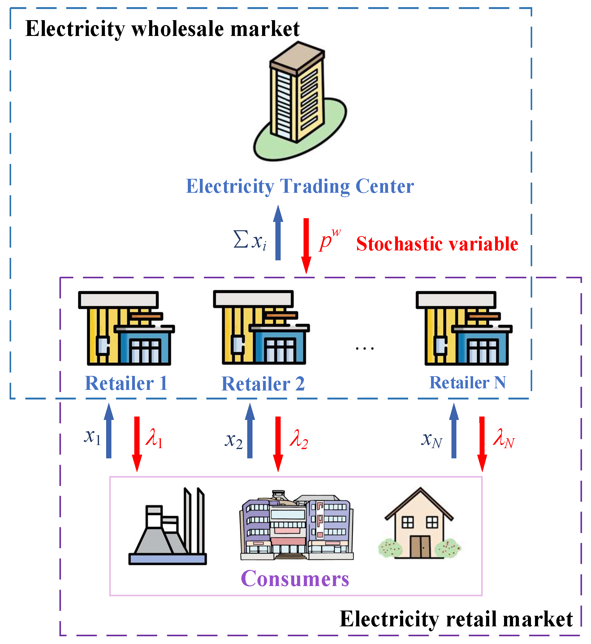
• By utilizing an open information network and smart home technologies in the deregulated electricity market [32], it can be predicted that intelligent consumers will have the ability to switch retailers in real time in the future. Therefore, we consider that multiple price-making retailers participate in the retail market competition, from which consumers will choose and switch their electricity supplies during a single time period (1 h).
• As shown in Figure 1, retailers are intermediaries between the electricity wholesale market and consumers. In the wholesale market, retailers purchase electricity at wholesale price. Because the competition in the wholesale market is unpredictable, the wholesale price is treated as a stochastic variable. In the retail market, retailers sell what they buy to consumers. Through the bidding process, retailers send the retail prices to customers, and the customers should send the load to retailers.

Defining $\mathit{I}=(1,\dots ,n)$ as the set of retailers, let $N=\left|\mathit{I}\right|$ denote the number of retailers. We discussed that electricity retail competition is based on price, so the decision variable of each retailer is the retail bidding price. $\mathit{\lambda }=\left({\lambda }_1,{\lambda }_2,\cdots ,{\lambda }_N\right)$ is a profile of individual retailers’ price bidding strategies, and ${\mathit{\lambda }}_{-i}$ represents the profile of retailers’ price bidding strategies, except for retailer i. Let $\mathit{x}=\left(x_1,x_2,\cdots ,x_N\right)$ be a profile of retailers’ retail loads, and let ${\mathit{x}}_{-i}$ denote the profile of retailers’ retail loads, except for retailer i. Then retailer $i\prime s\left(i\in \mathit{I}\right)$ decision-making process is as follows:

• During the retail bidding process, retailer $i$ offers retail bidding price ${\lambda }_i$ to realize its profit maximization. Once the profile of all retailers’ bidding prices, $\mathit{\lambda }$, is announced, consumers will adjust their demands. Accordingly, the retail load of retailer $i$ will change.
• Once retailer $i\prime s$ retail load is derived, retailer $i$ will purchase $x_i$ from the electricity wholesale market at wholesale price, $p^w$, which is a stochastic parameter, to supply the consumers’ demand.

Retailer $i(i\in \mathit{I})$’s profit consists of two parts. One is the revenue from sales to consumers in the retail market. The other is the purchase cost in the wholesale market, which is given by the following:

$$R_i={\lambda }_i{x}_i-p^w{x}_i$$

(1)

Assuming that the stochastic variable $p^w$ follows a probability distribution with a mean value, ${\mu }_w$, and a standard deviation, ${\sigma }_w$, it is not difficult to obtain the mean and variance of retailer $i$’s profit:

$${E(R}_i)={\lambda }_i{x}_i-{\mu }_w{x}_i$$

(2)

and

$${\sigma }^2\left(R_i\right)={\sigma }_w^2{x}_i^2$$

(3)

In order to capture the price elasticity and switching behavior of consumers in the retail market, retail prices offered by all retailers should be considered in the MSF of each retail. To formulate this, assume there is a fictional representative consumer on the electricity retail market who decides the retail load for all retailers in order to maximize the total return [21]. Then the MSF can be derived as follows:

$$x_i\left({\lambda }_i,{\mathit{\lambda }}_{-i}\right)=\sum _{j\in \mathit{I}}{\beta }_{i,j}{a}_j-{\beta }_i{\lambda }_i+\sum _{j\in \mathit{I},j\ne i}\left(-{\beta }_{i,j}\right){\lambda }_j$$

(4)

where $a_i>0$, ${\beta }_i>0$, and ${\beta }_{i,j}\le 0$. Specifically, the first term in (4), which is $\sum _{j\in \mathit{I}}{\beta }_{i,j}{a}_j>0$, represents retailer $i\prime s$ potential size [34]. ${\beta }_i$ indicates that the increase in retailer $i$’s bidding price will result in a drop in consumers’ demand, namely retailer $i$’s retail load. ${\beta }_{i,j}(j\ne i)$ is the switching factor which would interconnect the decision-making problems of all retailers.

${\beta }_{i,j}<0$ means consumers have switching behavior between retailer $i$ and $j$. For example, if retailer $j$ increases its retail price, consumers will switch a portion of their reduced demand from retailer $j$ to $i$, which will lead to a rise of retailer $i$’s retail load. We assume that ${\beta }_{i,j}={\beta }_{j,i}$, and a larger $\left|{\beta }_{i,j}\right|$ implies a greater consumer switching potential.

If ${\beta }_{i,j}=0$, which means consumers have no switching potential between retailer $i$ and $j$, retailer $i$’s MSF can be reformulated as follows:

$$x_i\left({\lambda }_i\right)={\beta }_i{a}_i-{\beta }_i{\lambda }_i$$

(5)

It can be found from (5) that, without considering consumers’ switching behavior, retailer $i\prime s$ retail load only depends on its own bidding price and parameters. By varying the values of $a_i$ and ${\beta }_i$, we can distinguish between retailers. For instance, if the retailer has a relatively high reputation and a large number of customers, the size, ${\beta }_i{a}_i$, of the potential market will be larger, and sensitivity parameter ${\beta }_i$ will be smaller to some extent, which means that this retailer may not easily lose consumers by incrementing its bid.

Furthermore, the parameters in (4) need to satisfy ${\beta }_i>\sum _{j=1,j\ne i}^N\left|{\beta }_{i,j}\right|$ and ${\beta }_i>\sum _{j=1,j\ne i}^N\left|{\beta }_{j,i}\right|$, which indicate that a per-unit increase in the bids offered by all retailers is not going to increase consumers’ demand to retailer i. In another words, a per-unit decrease in the bids offered by all retailers is not going to decrease consumers’ demand to retailer i when other parameters in (4) remain unchanged [21].

2.2. Game Model

Higher profit is usually accompanied by a higher risk. Thus, retailers have to consider the corresponding risks while maximizing their profits in the retail competition. To this end, each retailer aims to seek two goals. One is to maximize its profits, and the other is to minimize the corresponding risk; unfortunately, these two things conflict with each other. Indeed, how to balance the profit and risk depends on the retailer’s risk preference. Retailer i’s optimization problem can be expressed as a utility-maximization problem, as the follows, by using the mean–variance utility theory [35]:

$$\underset{{\lambda }_i}{\max }{U}_i=\left(1-r_i\right)E\left(R_i\right)-r_i{\sigma }^2\left(R_i\right)$$

(6)

where $U_i$ and $r_i$ are the utility function and risk preference of retailer $i$, respectively. Specifically, $r_i=0$ represents that retailer $i$ is risk-neutral, and $0{<r}_i<1$ represents that retailer $i$ is risk-averse; meanwhile, the higher $r_i$ representsthe more risk-averse retailer $i$ is.

Above all, retailer $i$’s optimization problem in the retail market can be expressed as follows:

$$\underset{{\lambda }_i}{\max }{U}_i\left({\lambda }_i,{\mathit{\lambda }}_{-i}\right)=\left(1-r_i\right)\left({\lambda }_i{x}_i-{\mu }_w{x}_i\right)-r_i{\sigma }_w^2{x}_i^2$$

(7)

$$\mathrm{s}.\mathrm{t}.{\lambda }_i^{min}\le {\lambda }_i\le {\lambda }_i^{max}$$

(8)

$$x_i\left({\lambda }_i,{\mathit{\lambda }}_{-i}\right)=\sum _{j\in \mathit{N}}{\beta }_{i,j}{a}_j-{\beta }_i{\lambda }_i+\sum _{j\in \mathit{N},j\ne i}\left(-{\beta }_{i,j}\right){\lambda }_j$$

(9)

It can be found that the utility of each retailer depends on both its own bidding price and the bids of its competitors. Thus, by gathering all individual retailer’s optimization problems, (7)–(9), the game model of this paper can be obtained, considering that the price bidding among retailers in the retail market is a one-time game and there is no cooperation among retailers.

Definition 1. 

In our research, we define the retail market game model as $G=\left\{I,{\left({\lambda }_i\right)}_{i\in I},{\left(U_i\right(\lambda )}_{i\in I}\right\}$.

Definition 2. 

For the game problem, $G$, the profile of retailers’ strategy, ${\mathit{\lambda }}^{*}=({\lambda }_1^{*},{\lambda }_2^{*},\cdots {,\lambda }_N^{*})$, is an Nash equilibrium if and only if $U_i({\lambda }_i^{*},{\mathit{\lambda }}_{-i}^{*})\ge U_i({\lambda }_i,{\mathit{\lambda }}_{-i}^{*})$ for all $i\in \mathit{I}$ and any ${\lambda }_i\in {\Omega }_i=\left\{{\lambda }_i|{\lambda }_i^{min}\le {\lambda }_i\le {\lambda }_i^{max}\right\}$.

2.3. Existence and Uniqueness of Nash Equilibrium

Note that the Nash equilibrium will always exist and remain unique in a general noncooperative game. Therefore, we should investigate whether the proposed game model contains a unique Nash equilibrium in our paper.

Theorem 1. 

There must be more than one pure strategy Nash equilibrium in the game problem, $G$.

Proof. 

According to [36], a pure strategy Nash equilibrium exists in the game if the following two conditions hold:

• Each retailer’s strategy space is closed, bounded, and convex.
• In regard to the retailer’s strategy of its own, its profit function is continuous and quasi-concave.

From Definition 2, it is easy to know that retailer $i\prime s\left(i\in \mathit{I}\right)$ strategy space, ${\mathsf{\Omega }}_i$, is an enclosed and convex set with clear boundaries. So, Condition 1 is satisfied.

In regard to ${\lambda }_i$, we take the first and second derivatives of $U_i\left(\mathit{\lambda }\right)$ and obtain the following:

$$\frac{\partial U_i\left(\mathit{\lambda }\right)}{\partial {\lambda }_i}=\left(1-r_i+2{\beta }_i{r}_i{\sigma }_w^2\right)\left[{\beta }_i\left(a_i-{\lambda }_i\right)+\sum _{j\in \mathit{N},j\ne i}{\beta }_{i,j}\left(a_j-{\lambda }_j\right)\right]-{\beta }_i\left(1-r_i\right)\left({\lambda }_i-{\mu }_w\right)$$

(10)

$$\frac{{\partial }^2{U}_i\left(\mathit{\lambda }\right)}{\partial {\lambda }_i^2}=-2{\beta }_i\left(1-r_i+{\beta }_i{r}_i{\sigma }_w^2\right)$$

(11)

From (10), we can obtain a continuous utility function for retailer $i$. Owing to ${\beta }_i>0$ and ${0<r}_i<1$, the right-hand side of (11) is negative. In terms of its strategy space, the utility function, $U_i\left(\mathit{\lambda }\right)$, of retailer $i$ is strictly concave and is therefore a quasiconcave function. Consequently, Condition 2 is satisfied.

In conclusion, the game problem, $G$, has at least one pure strategy Nash equilibrium. □

Theorem 2. 

The game problem, $G$, has a unique Nash equilibrium.

Proof. 

In accordance with [36], the proposed game model has a unique NE if each retailer’s best response mapping is a contraction of its entire strategy space.

In the game, considering the strategies of the other retailers, ${\mathit{\lambda }}_{-i}$, we find that the best response function for retailer $i$ is the best strategy for retailer $i$. Thus, we obtain the following:

$${\lambda }_i\left({\mathit{\lambda }}_{-i}\right)=\arg \underset{{\lambda }_i}{\max }{U}_i\left({\lambda }_i,{\mathit{\lambda }}_{-i}\right)$$

(12)

In order to calculate the derivative of (10), we need to take the derivative with respect to ${\lambda }_j$, and we obtain the following:

$$\frac{{\partial }^2{U}_i\left(\mathit{\lambda }\right)}{\partial {\lambda }_i\partial {\lambda }_j}=-{\beta }_{i,j}\left(1-r_i+{2\beta }_i{r}_i{\sigma }_w^2\right)$$

(13)

In order to determine the first-order derivative of retailer $i$’s ${\lambda }_i\left({\mathit{\lambda }}_{-i}\right)$ when compared to its rival’s bidding price, ${\lambda }_j(j\ne i)$, we can apply the implicit function theorem as follows:

$$\frac{\partial {\lambda }_i\left({\mathit{\lambda }}_{-i}\right)}{\partial {\lambda }_j}=-\frac{\frac{{\partial }^2{U}_i\left(\mathit{\lambda }\right)}{\partial {\lambda }_i\partial {\lambda }_j}}{\frac{{\partial }^2{U}_i\left(\mathit{\lambda }\right)}{\partial {\lambda }_i^2}}=-\frac{{\beta }_{i,j}}{{\beta }_i}·\frac{1-r_i+{2\beta }_i{r}_i{\sigma }_w^2}{2\left(1-r_i\right)+{2\beta }_i{r}_i{\sigma }_w^2}$$

(14)

Due to ${\beta }_i>-{\beta }_{i,j}>0$, we have the following:

$$0<\partial {\lambda }_i\left({\mathit{\lambda }}_{-i}\right)/\partial {\lambda }_j<1$$

(15)

In conclusion, a contract mapping is the best response function of retailer $i$ since it satisfies $\left|\partial {\lambda }_i\left({\mathit{\lambda }}_{-i}\right)/\partial {\lambda }_j\right|<1$ [36]. Thus, Theorem 2 is proved: there exists a unique Nash equilibrium in the game problem, $G$. □

2.4. Impacts of the Uncertainty of Wholesale Price Uncertainty and Risk Preference on Retailer’s Bidding Strategy

For the convenience of theoretical analysis, the inequality constraint condition (8) are not considered her; however, this does not impact the analysis results. Substituting (5) into (7), in the decision-making problem of retailer $i$, the optimal first-order condition is as follows:

$$\frac{\partial U_i}{\partial {\lambda }_i}=\left(1-r_i+2{\beta }_i{r}_i{\sigma }_w^2\right)\left(a_i-{\lambda }_i\right){\beta }_i-{\beta }_i\left(1-r_i\right)\left({\lambda }_i-{\mu }_w\right),\forall i\in \mathit{I}$$

(16)

From (16), we can obtain the optimal bidding price of retailer $i$, which is as follows:

$${\lambda }_i=\frac{\left(1-r_i+2{\beta }_i{r}_i{\sigma }_w^2\right)+\left(1-r_i\right){\mu }_w}{2\left(1-r_i+{\beta }_i{r}_i{\sigma }_w^2\right)}$$

(17)

Then, retailer $i$’s retail load, expected profit, and variance of profit are, respectively, calculated as follows:

$$x_i=\frac{\left(1-r_i\right)\left(a_i-{\mu }_w\right){\beta }_i}{2\left(1-r_i+{\beta }_i{r}_i{\sigma }_w^2\right)}$$

(18)

$$E\left(R_i\right)=\frac{{\left(a_i-{\mu }_w\right)}^2\left(1-r_i+2{\beta }_i{r}_i{\sigma }_w^2\right)\left(1-r_i\right){\beta }_i}{4{\left(1-r_i+{\beta }_i{r}_i{\sigma }_w^2\right)}^2}$$

(19)

$${\sigma }^2\left(R_i\right)={\sigma }_w^2{\left[\frac{\left(1-r_i\right)\left(a_i-{\mu }_w\right){\beta }_i}{2\left(1-r_i+{\beta }_i{r}_i{\sigma }_w^2\right)}\right]}^2$$

(20)

From (18)–(20), the first-order partial derivative of the retail price, retail load, expected profit, and variance of profit of retailer $i$ with respect to ${\sigma }_w^2$ can be acquired as follows:

$$\frac{\partial {\lambda }_i}{\partial {\sigma }_w^2}=\frac{{\beta }_i{r}_i\left(1-r_i\right)\left(a_i-{\mu }_w\right)}{2{\left(1-r_i+r_i{\sigma }_w^2{\beta }_{\dot{i}}\right)}^2}$$

(21)

$$\frac{\partial x_i}{\partial {\sigma }_w^2}=\frac{\left(1-r_i\right)\left(a_i-{\mu }_w\right){\beta }_i^2{r}_i}{2{\left(1-r_i+{\beta }_i{r}_i{\sigma }_w^2\right)}^2}$$

(22)

$$\frac{\partial E\left(R_i\right)}{\partial {\sigma }_w^2}=-\frac{{\left(a_i-{\mu }_w\right)}^2\left(1-r_i\right){\beta }_i^3{r}_i^2{\sigma }_w^2}{2{\left(1-r_i+{\beta }_i{r}_i{\sigma }_w^2\right)}^3}$$

(23)

$$\frac{\partial {\sigma }^2\left(R_i\right)}{\partial {\sigma }_w^2}={\left[\frac{\left(1-r_i\right)\left(a_i-{\mu }_w\right){\beta }_i}{2\left(1-r_i+{\beta }_i{r}_i{\sigma }_w^2\right)}\right]}^2\left(\frac{1-r_i-{\beta }_i{r}_i{\sigma }_w^2}{1-r_i+{\beta }_i{r}_i{\sigma }_w^2}\right)$$

(24)

It can be found from (21)–(24) that $\partial {\lambda }_i/\partial {\sigma }_w^2>0$, $\partial x_i/\partial {\sigma }_w^2<0$, and $\partial E\left(R_i\right)/\partial {\sigma }_w^2<0$, which demonstrate when the uncertainty of wholesale price increases (i.e., a larger variance), and the retailer will increase its retail bidding price, and both its retail load and expected profit will decrease. From (24), it can be found that $\partial {\sigma }^2\left(R_i\right)/\partial {\sigma }_w^2>0$ when ${\sigma }_w^2<(1-r_i)/{\beta }_i{r}_i$; namely, the variance of retailer’s profit will increase with the increase in the variance of wholesale price. Moreover, $\partial {\sigma }^2\left(R_i\right)/\partial {\sigma }_w^2<0$ when ${\sigma }_w^2>(1-r_i)/{\beta }_i{r}_i$; namely, the variance of retailer’s profit will decrease with the increase in the variance of wholesale price.

The first-order partial derivatives of retailer $i$’s bidding price, retail load, expected profit, and standard deviation of profit with respect to its risk preference, $r_i$, are further examined as follows.

$$\frac{\partial {\lambda }_i}{\partial r_i}=\frac{\left(a_i-{\mu }_w\right){\beta }_i{\mathsf{\sigma }}_w^2}{2{\left(1-r_i+r_i{\sigma }_w^2{\beta }_i\right)}^2}$$

(25)

$$\frac{\partial x_i}{\partial r_i}=\frac{\left(a_i-{\mu }_w\right){\beta }_i{\mathsf{\sigma }}_w^2}{2{\left(1-r_i+{\beta }_i{r}_i{\sigma }_w^2\right)}^2}$$

(26)

$$\frac{\partial E\left(R_i\right)}{\partial r_i}=-\frac{{\left(a_i-{\mu }_w\right)}^2{\beta }_i^3{r}_i{\sigma }_w^4}{2{\left(1-r_i+{\beta }_i{r}_i{\sigma }_w^2\right)}^3}$$

(27)

$$\frac{\partial \sigma \left(R_i\right)}{\partial r_i}=-\frac{\left(a_i-{\mu }_w\right){\beta }_i^3{\sigma }_w^3}{2{\left(1-r_i+{\beta }_i{r}_i{\sigma }_w^2\right)}^2}$$

(28)

It can be seen from (25)–(28) that $\partial {\lambda }_i/\partial r_i>0$, $\partial x_i/\partial r_i<0$, $\partial E\left(R_i\right)/\partial r_i<0$, and $\partial \sigma \left(R_i\right)/\partial r_i<0$, which show that the increase in the risk-averse level of retailer $i$ will lead to the increase in its retail price and the decrease in its retail load, expected profit, and standard deviation of profit.

2.5. Solution Method

The Nash equilibrium of the game model, G, mentioned above can be attained by collecting the optimization issues of each retailer and then solving them simultaneously. Note that the Nash equilibrium ${\mathit{\lambda }}^{\mathrm{*}}=({\lambda }_1^{\mathrm{*}},{\lambda }_2^{\mathrm{*}},\cdots {,\lambda }_N^{\mathrm{*}})$ should fulfill the Karush–Kuhn–Tucker (KKT) conditions [12,37] of each retailer’s optimization problem.

The KKT conditions of retailer $i\left(i\in \mathit{I}\right)$ are calculated as follows.

$$\left({\lambda }_i,\forall i\right):\left(1-r_i+2{\beta }_i{r}_i{\sigma }_w^2\right)\left[{\beta }_i\left(a_i-{\lambda }_i\right)+\sum _{j\in \mathit{N},j\ne i}{\beta }_{i,j}\left(a_j-{\lambda }_j\right)\right]-{\beta }_i\left(1-r_i\right)\left({\lambda }_i-{\mu }_w\right)+{\mu }_{1i}-{\mu }_{2i}$$

(29)

$$\left({\mu }_{1i},\forall i\right):{\mu }_{1i}\ge 0,\left({\lambda }_i-{\lambda }_i^{min}\right)\ge 0,{\mu }_{1i}\left({\lambda }_i-{\lambda }_i^{min}\right)=0$$

(30)

$$\left({\mu }_{2i},\forall i\right):{\mu }_{2i}\ge 0,\left({\lambda }_i^{max}-{\lambda }_i\right)\ge 0,{\mu }_{2i}\left({\lambda }_i^{max}-{\lambda }_i\right)=0$$

(31)

where ${\mu }_{1i}$ and ${\mu }_{2i}$ represent the lower and upper bounds of retailer $i$’s retail price, respectively.

We can obtain the equilibrium outcomes by solving the problem of all retailers’ KKT conditions simultaneously. However, it can be seen that the complementarity conditions, such as (30) and (31), are included in each retailer’s KKT conditions. By adopting the nonlinear complementarity method [12], expressions (30) and (31) can be reformulated as nonlinear equations, as shown in (32) and (33):

$$\left({\mu }_{1i},\forall i\right):{\mu }_{1i}+{\lambda }_i-{\lambda }_i^{min}-\sqrt{{\mu }_{1i}^2+{\left({\lambda }_i-{\lambda }_i^{min}\right)}^2}=0$$

(32)

$$\left({\mu }_{2i},\forall i\right):{\mu }_{2i}+{\lambda }_i^{max}-{\lambda }_i-\sqrt{{\mu }_{2i}^2+{\left({\lambda }_i^{max}-{\lambda }_i\right)}^2}=0$$

(33)

Accordingly, a group of nonlinear algebraic equations is generated from the KKT conditions of each retailer’s optimization problem. Using the Levenberg–Marquardt algorithm, the Nash equilibrium of the game problem, G, can be derived by solving the nonlinear equation sets of all retailers.

3. Numerical Examples

3.1. Impacts of Wholesale Price Uncertainty on Equilibrium Outcomes

Given the fact that retail prices offered by retailers are highly linked to the wholesale price in the real-time pricing scheme, the impacts of wholesale price uncertainty are firstly discussed. Assume that two symmetric retailers participate in the retail competition. The parameters in each retailer’s MSF are $a_i=80$ $/MWh, ${\beta }_i=16$ (MW)² h/$, and $\left|{\beta }_{i,j}\right|=2$ (MW)² h/$ ($i,j=1,2$ and $i\ne j$). The electricity wholesale price follows a lognormal distribution, with a mean value of ${\mu }_w=60$ $/MWh and a standard deviation, ${\sigma }_w$. It should be noted that the data defined in MSF coefficients are an academic exercise, not realistic [34].

When the two retailers are risk-neutral, i.e., $r_1=r_2=0$, their equilibrium retail prices, retail loads, and expected profits are 69.33 $/MWh, 149.33 MW, and 1.394 × 10³ $/MWh, respectively. These equilibrium outcomes remain unchanged when the uncertainty of wholesale price varies (i.e., with different standard deviation values).

Furthermore, considering that the two retailers have risk-averse characteristics. Their risk-preference coefficients are r₁ = 0.05 and r₂ = 0.10, meaning that the risk-averse level of Retailer 2 is relatively larger.

Table 1. Impacts of the standard deviation of wholesale price on equilibrium outcomes.

Equilibrium Outcomes	${\mathit{\sigma }}_{\mathit{w}}$ = 0.2	${\mathit{\sigma }}_{\mathit{w}}$ = 0.4	${\mathit{\sigma }}_{\mathit{w}}$ = 0.6
${\lambda }_1$ ($/MWh)	69.68	70.59	71.80
$x_1$ (MW)	145.09	133.51	117.55
$E\left(R_1\right)$ (103 $/h)	1.404	1.414	1.387
$\sigma \left(R_1\right)$ ($/h)	29.02	53.40	70.53
${\lambda }_2$ ($/MWh)	69.98	71.50	73.19
$x_2$ (MW)	139.74	117.24	92.56
$E\left(R_2\right)$(103 $/h)	1.394	1.348	1.221
$\sigma \left(R_2\right)$ ($/h)	27.95	46.90	55.54
Total demand (MW)	284.83	250.75	210.11

shows the equilibrium outcomes under different ${\sigma }_w$ values. It can be seen that, with the increase in ${\sigma }_w$, the retail prices provided by the two retailers will increase and the retailer loads of the two retailers will decrease. Moreover, in the case of the same ${\sigma }_w$, Retailer 2, with a relatively higher risk-averse level, will offer a relatively higher retail price than Retailer 1. Meanwhile, the expected profit of Retailer 2 and the standard deviation of Retailer 2’s profit are relatively smaller. These results are consistent with the theoretical analysis in Section 2.4.

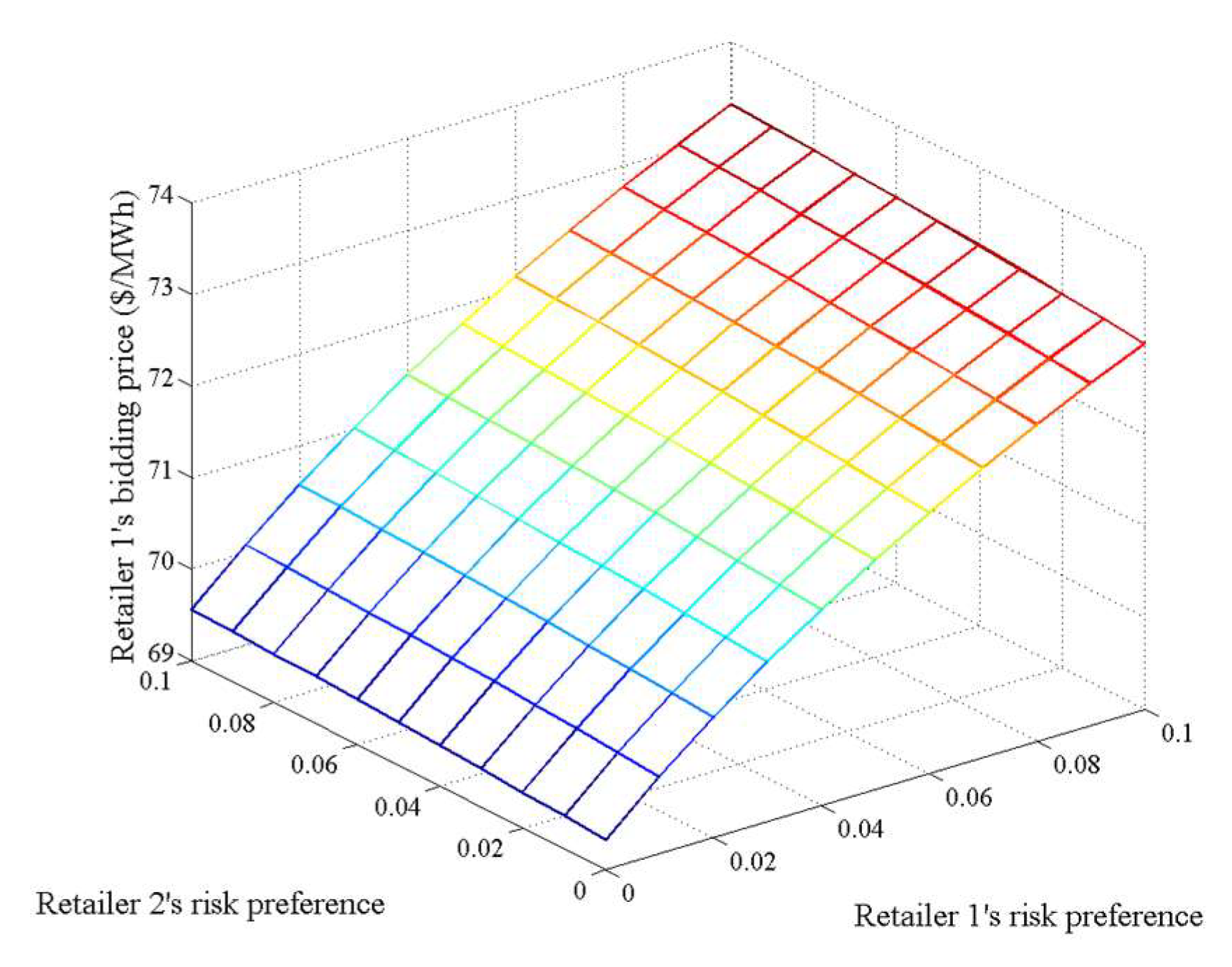
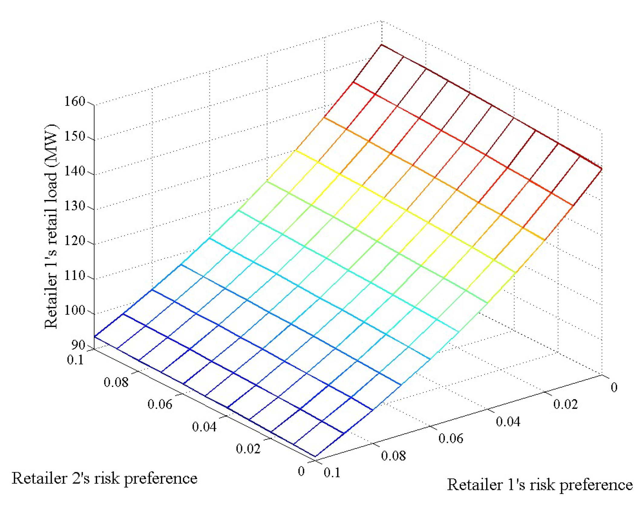
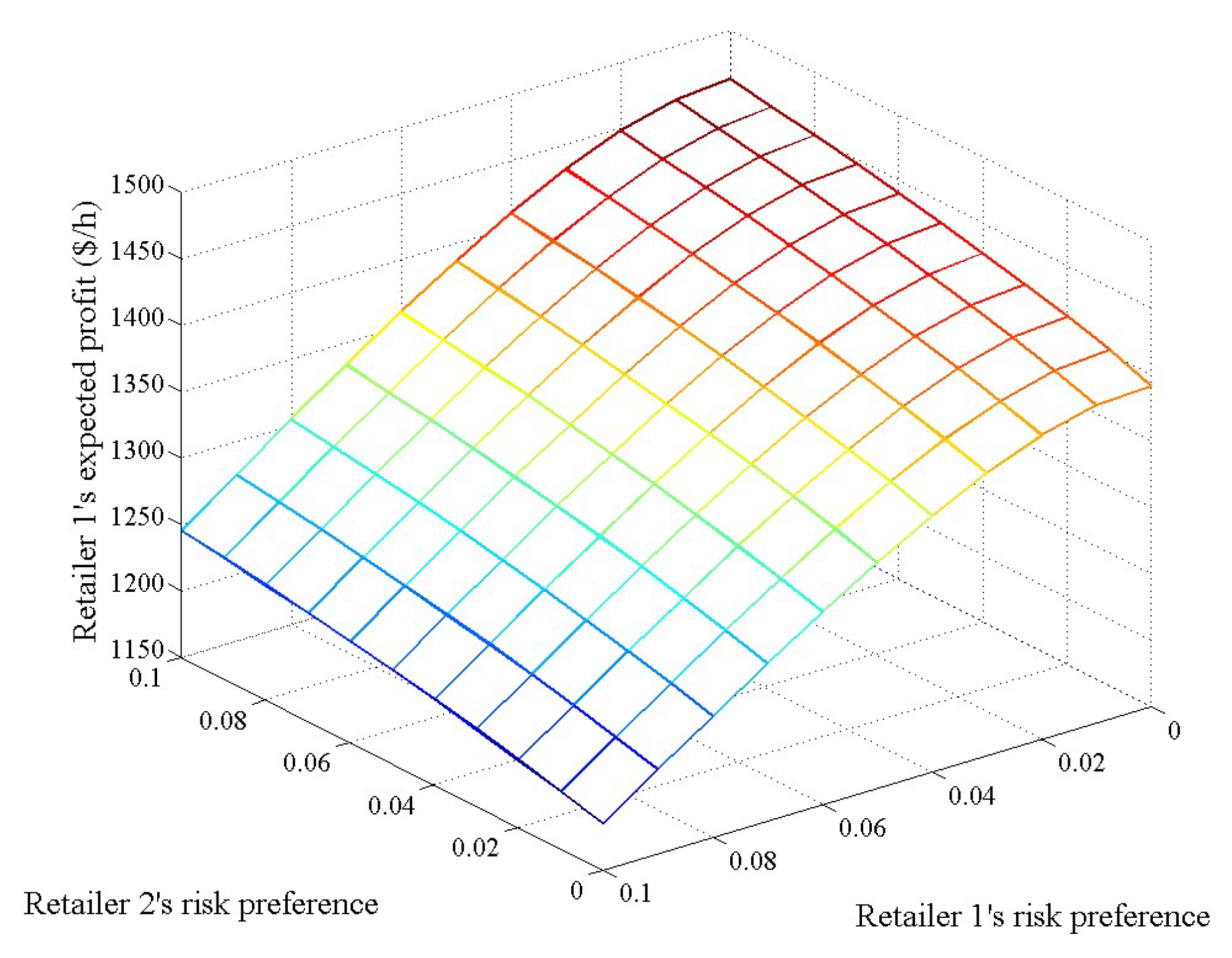
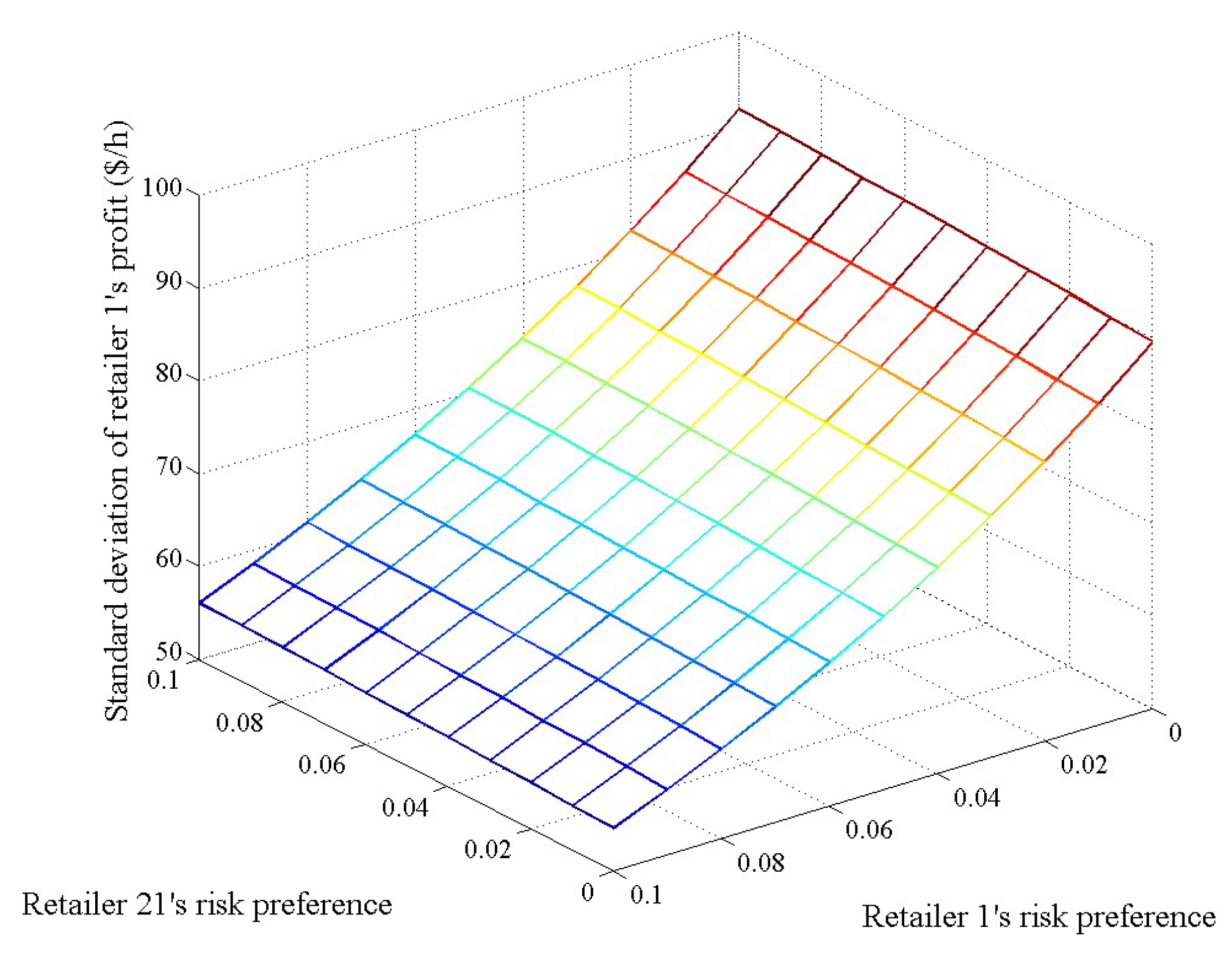
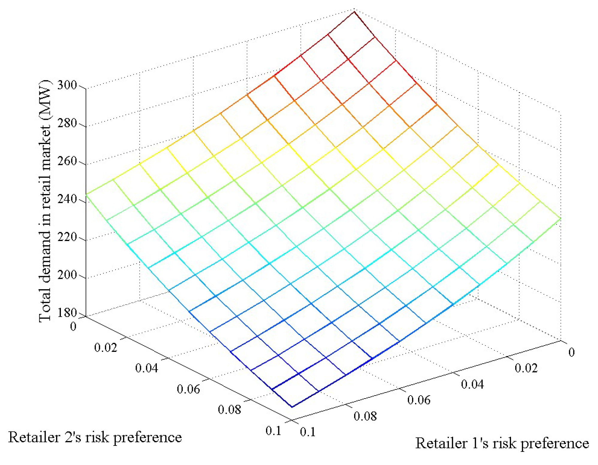
3.2. Impacts of Retailers’ Risk Preferences on Equilibrium Outcomes

Considering the fact that the electricity retail market is more akin to oligopoly in many countries, it is significant to analyze the strategic bidding of retailers by oligopoly equilibrium models. Meanwhile, given the fact that different retailers have different risk preferences, the change of one retailer’s risk preference not only affects its own bidding strategy and utility but also affect its rivals’ bidding strategies and utilities. In order to display the interaction, numerical simulations are conducted as follows, which can help policymakers to find the market power issues.

Assume that the mean value and standard deviation of the electricity wholesale price are ${\mu }_w=60$ $/MWh and ${\sigma }_w=0.6$ $/MWh, respectively. The parameters in two symmetric retailers’ MSFs are the same as those in Section 3.1. Figure 2, Figure 3, Figure 4 and Figure 5 show the impacts of two retailers’ risk preferences on Retailer 1’s equilibrium retail price, retail load, the expected profit, and the standard deviation of profit, respectively.

It can be found from Figure 2, Figure 3 and Figure 4 that, with the increase in Retailer 1’s risk-averse level, its bidding price will go up, while its retail load, expected profit, and standard deviation of profit will decrease. These results are consistent with the theoretical analysis in Section 2.4.

It can be seen from Figure 2 that Retailer 1 will raise its bidding price with the increase in its rival’s (i.e., Retailer 2’s) risk-averse level. It also can be seen that, with the increase in Retailer 2’s risk-averse level, its own bidding price will increase, as discussed in Section 2.4. Meanwhile, the magnitude of the increase in Retailer 2’s bidding price is significantly larger than that of Retailer 1, as shown in Figure 2. As such, with the increase in Retailer 2’s risk-averse level, the bidding price of Retailer 2 will be higher than that of Retailer 1, and this will incentivize consumers to reduce the demand from Retailer 2 and switch to Retailer 1. Therefore, Retailer 1’s retail load will increase with the increase in its rival’s risk-averse level, as shown in Figure 3.

To sum up, the retail bidding price of a retail will increase not only with the increase in its own risk-averse level but also with the increase in its rival’s risk-averse level, and the retail price is more affected by its own risk-averse level. Moreover, it can be concluded that, with the increase in a retailer’s risk-averse level, its own retail load will drop, and its rival’s retail load will increase. As a result of its own retail load decreasing more than the competitors’ retail loads increasing, the total retail demand in the retail market decreased, as shown in Figure 6.

From Figure 4 and Figure 5, it can be observed that a retailer’s expected profit and standard deviation of profit will decrease with the increase in its own risk-averse level and increase with the increase in its rival’s risk-averse level. In other words, increasing the risk-averse level of a retailer itself will reduce the risk of its profit, but increasing the risk-averse level of its rival may have an adverse effect on the risk of its profit.

The above results also indicate that, for a certain retailer, when its rival retailer’s risk-averse level goes up, this retailer may have a chance to enhance the retail bidding price by bidding more strategically, occupy a larger market share, and make more profit.

We further consider three asymmetrical retailers participating in the retail competition. As mentioned in Section 2.1, there are three retailers that can be distinguished by $a_i$ and ${\beta }_i$, as indicated in

Table 2. Parameters in MSFs.

Retailer	${\mathit{a}}_{\mathit{i}}$ ($/MWh)	${\mathit{\beta }}_{\mathit{i}}$ ((MW)2 h/$)
1	80	20
2	90	18
3	100	17

. It can be found from Table 2 that Retailer 3 has a fairly higher reputation and larger consumer base than Retailers 1 and 2. Meanwhile, assuming that the switching factor in each retailer’s MSF is $\left|{\beta }_{i,j}\right|=2$ (MW)² h/$ ($i,j=1,2,3$ and $i\ne j$), let Retailers 1 and 2 be risk-neutral.

Table 3. Impacts of Retailer 3’s risk preference on equilibrium outcomes.

r3	Retailer	${\mathit{\lambda }}_{\mathit{i}}$ ($/MWh)	${\mathit{x}}_{\mathit{i}}$ (MW)	$\mathit{E}\left({\mathit{R}}_{\mathit{i}}\right)$ (103$/h)	$\mathit{\sigma }\left({\mathit{R}}_{\mathit{i}}\right)$ ($/h)
0	1	68.07	161.44	1.303	96.86
	2	73.13	236.38	3.104	141.83
	3	78.31	311.20	5.695	186.72
0.05	1	68.31	166.20	1.381	99.72
	2	73.40	241.11	3.230	144.67
	3	82.80	235.76	5.376	141.46
0.10	1	68.47	169.35	1.434	101.61
	2	73.57	244.25	3.314	146.55
	3	85.78	185.78	4.789	111.44

shows the equilibrium outcomes when Retailer 3’s risk preference equals 0, 0.05, and 0.1.

From Table 3, it can be observed that, with the increase in the risk-averse level of Retailer 3, its retail bidding price will increase, and its expected profit, retail load, and standard deviation of profit will decrease. Meanwhile, affected by the increase in Retailer 3’s risk-averse level, retail prices supplied by Retailers 1 and 2 will increase. Moreover, Retailers 1 and 2’s loads are increased because of consumers’ switching behavior. That is, as Retailer 3’s bidding price is higher, consumers will switch a portion of their demands to be supplied by Retailers 1 and 2, whose bidding prices are lower than Retailer 3’s. Both Retailers 1 and 2’s expected profit and the standard deviation of profit will increase with the increase in Retailer 3’s risk-averse level. The above results are consistent with the aforementioned analysis under the symmetrical case.

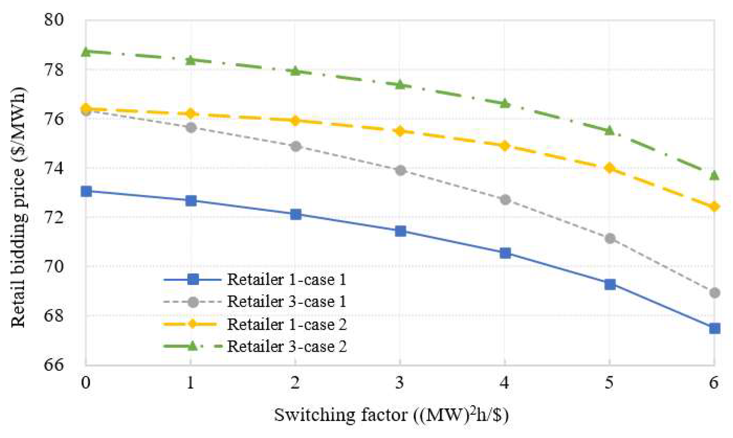
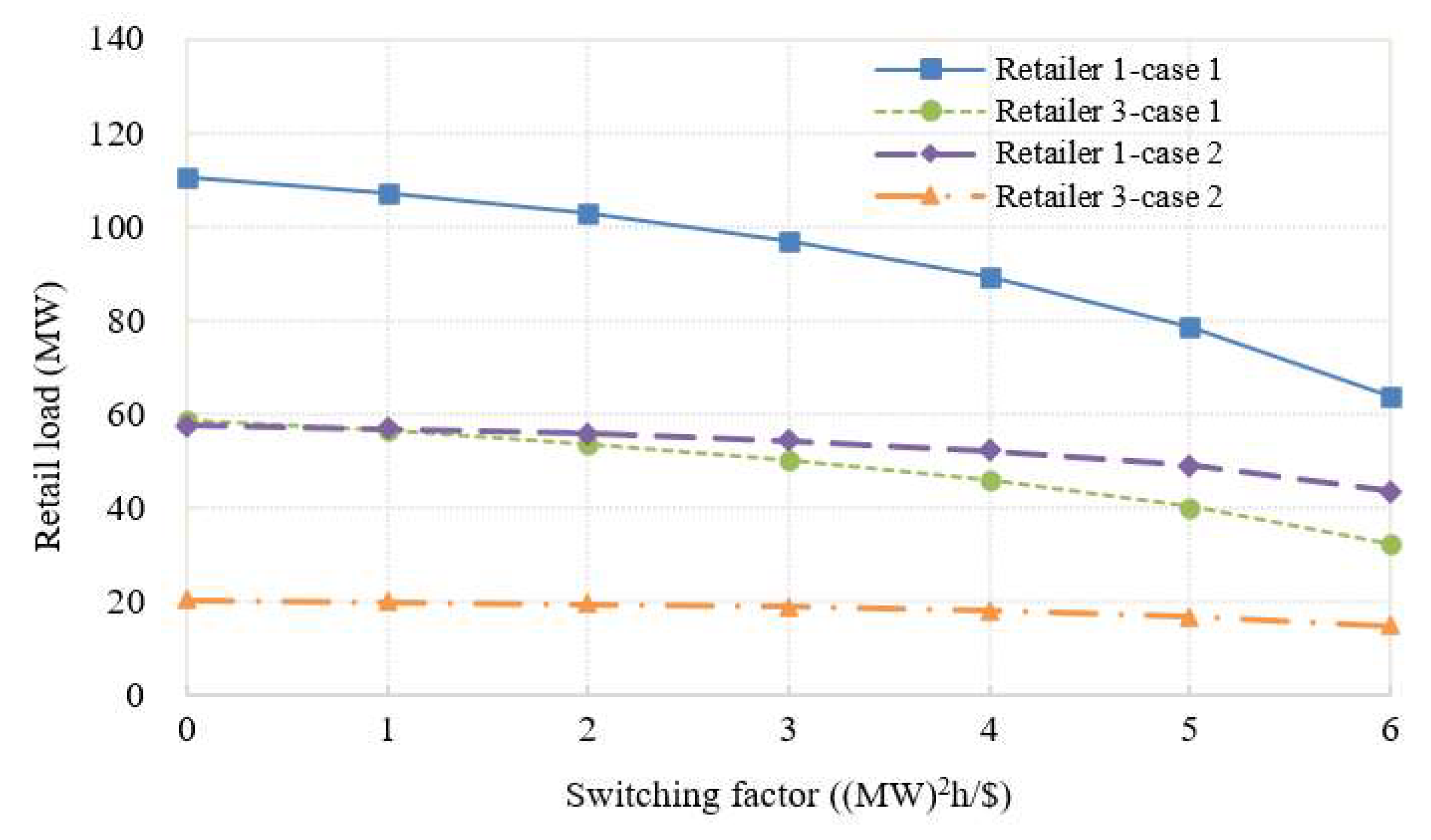
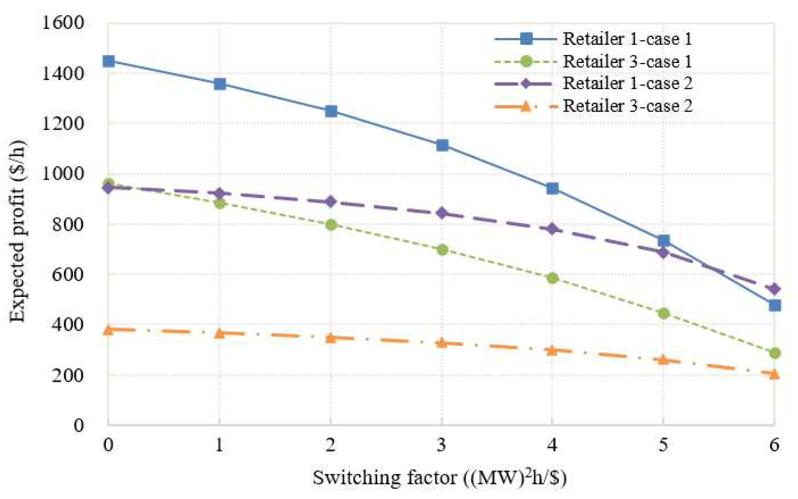
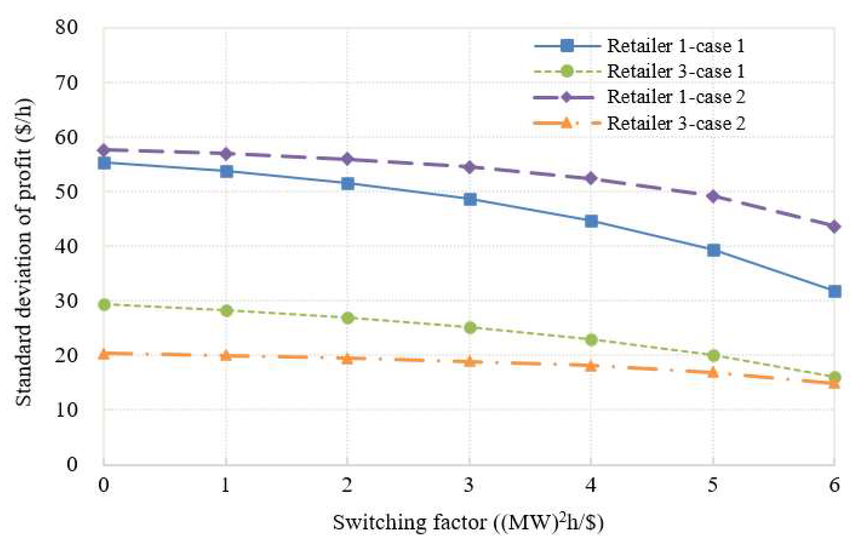
3.3. Impacts of Consumers’ Switching Behavior on Strategic Bidding Behaviors of Retailers with Different Risk-Averse Levels

As consumers will adjust their demand and/or switch retailers according to retail prices in the deregulated retail market, which will inevitably impact retailers’ bidding strategies in the retail market, integrating consumers’ elasticity and switching behaviors into the game analysis is significant. This section focuses on analyzing the impacts of consumers’ switching behavior on retailers’ price bidding strategies and equilibrium outcomes, with different standard deviations of the wholesale price.

Considering that three retailers with different risk-averse levels participate in the retail market competition, the parameters of each retailer’s MSF are $a_i=80$ $/MWh and ${\beta }_i=16$ (MW)² h/$ ($i=1,2,3$). Assume that three retailers are risk-averse and the risk-averse level of Retailer 3 is relatively higher, namely $r_1=0.10$, $r_2=0.20$, and $r_3=0.30$. In Case 1, the mean and the standard deviation are ${\mu }_w=60$ $/MWh ${\sigma }_w=0.5$ $/MWh, respectively. In Case 2, the standard deviation of the wholesale price is relatively larger, i.e., ${\sigma }_w=1.0$ $/MWh. For the sake of comparison and analysis, we take Retailers 1 and 3 as examples. Figure 7, Figure 8, Figure 9 and Figure 10 show the equilibrium outcomes of Retailers 1 and 3 in the two cases, with respect to switching factors $\left|{\beta }_{i,j}\right|$ ($i,j=1,2,3$ and $i\ne j$), including retail price, retail load, expected profit, and standard deviation of profit.

It can be seen from Figure 7 that the bidding prices of Retailers 1 and 3 will decrease as switching factors increase in both cases, thus demonstrating that consumers’ switching behavior can contribute to the mitigation of retailers’ market power abuse. Moreover, under the same ${\sigma }_w$, the magnitude of decrease in Retailer 3’s bidding price is larger than that of Retailer 1. In other words, the more risk-averse a retailer is, the more obvious the mitigative effect of consumers’ switching behavior on its market power will be.

The retail loads from Retailers 1 and 3 will drop with the increase in switching factors because the mitigation in the retailers’ market power will result in a fall in their willingness to offer electricity in the retail market [21], as shown in Figure 8. Accordingly, Retailers 1 and 3’s expected profits and standard deviations of profits will decrease as switching factors increase in both cases, as shown in Figure 9 and Figure 10.

Moreover, compared with the equilibrium outcomes in Case 1, it can be observed from Figure 7, Figure 8, Figure 9 and Figure 10 that, as switching factors increase, the magnitudes of decrease in Retailer 3’ bidding price, retail loads, expected profits, and standard deviations of profit are relatively smaller in Case 2. This can be explained via two reasons: One is because, although the increase in switching factors will decrease bidding prices, risk-averse retailers also need to maintain a certain level of bidding prices to hedge against the risk when facing in the higher uncertainty of the wholesale price. The other is due to the reduction of total demand, which is caused by the higher uncertainty of the wholesale price; retailers may show less willingness to attract consumers by decreasing their bidding prices. In other words, in the situation with relatively lower uncertainty of the wholesale price, the mitigative effect of consumers’ switching behavior on risk-averse retailers’ market power would be more significant.

4. Conclusions

Up until now, the research about the bidding strategies of retailers with different risk preferences in the electricity market with switchable consumers has been very limited. This paper considered the uncertainty of the wholesale price and how retailers with different risk preferences will have different strategic bidding behaviors in the electricity retail market. A game model of the electricity retail market was proposed, while considering retailers’ risk preferences and consumers’ switching behavior. Then the existence and uniqueness of the Nash equilibrium in the proposed model were theoretically proved. A theoretical analysis was presented to investigate the impacts of wholesale price uncertainty and risk preference on retailer’s bidding strategy. The effectiveness of the proposed model was illustrated through case studies.

The main findings and practical insights are summarized as follows:

• When risk-averse retailers participate in the retail market competition, every retailer’s bidding price will increase with the increase in the uncertainty of the wholesale price (i.e., a larger standard deviation). The more risk-averse the retailer is, the more obvious this effect will be.
• A retailer will raise its retail bidding price when the risk-averse levels of itself and its rivals increase, and it will be more affected by its own risk-averse level. Meanwhile, a retailer’s expected profit and standard deviation of profit will decrease with the increase in its own risk-averse level and increase with the increase in its rival’s risk-averse level. We also found that a retailer may have a chance to raise its bidding price, occupy a relatively larger market share, and make more profit by exercising market power when the risk-averse level of its rival retailer increases.
• Consumers’ switching behavior can help mitigate the strategic behaviors of retailers and lower the retail prices. Moreover, the more risk-averse the retailers are, the more obvious the mitigative effect of consumers’ switching behavior on their strategic behaviors will be. Moreover, in the case of a relatively lower uncertainty level of the wholesale price, consumers’ switching behavior may have a better mitigative effect on the market power of risk-averse retailers.

The above conclusions can provide reference for policymakers to address market power issues and improve the efficiency of the electricity retail market. Meanwhile, in the context of the high penetration of renewable energy power, analyzing bidding strategies of retailers with risk preference can help retailers to cope with risks and find a balance, and then promote the deregulation of the electricity market and the consumption of renewablepower. Future directions of this work can include modeling the renewable generators to better explain the interaction between wholesale price fluctuation and retailers’ bidding strategies.

References

1. Bao, M.; Ding, Y.; Zhou, X.; Guo, C.; Shao, C. Risk assessment and management of electricity markets: A review with suggestions. CSEE J. Power Energy Syst. 2021, 7, 1322–1333. [Google Scholar]
2. Fatras, N.; Ma, Z.; Duan, H.; Jørgensen, B.N. A systematic review of electricity market liberalisation and its alignment with industrial consumer participation: A comparison between the Nordics and China. Renew. Sustain. Energy Rev. 2022, 167, 112793. [Google Scholar] [CrossRef]
3. Tsai, C.; Tsai, Y. Competitive retail electricity market under continuous price regulation. Energy Policy 2018, 114, 274–287. [Google Scholar] [CrossRef]
4. Zare, K.; Nojavan, S.; Mohammadi-Ivatloo, B. Optimal bidding strategy of electricity retailers using robust optimisation approach considering time-of-use rate demand response programs under market price uncertainties. IET Gener. Transm. Distrib. 2015, 9, 328–338. [Google Scholar]
5. He, J.; Cai, L.; Cheng, P.; Fan, J. Optimal investment for retail company in electricity market. IEEE Trans. Ind. Inform. 2015, 11, 1210–1219. [Google Scholar] [CrossRef]
6. Mohammad, N.; Mishra, Y. Retailer’s risk-aware trading framework with demand response aggregators in short-term electricity markets. IET Gener. Transm. Distrib. 2019, 13, 2611–2618. [Google Scholar] [CrossRef]
7. Woo, C.K.; Zarnikau, J.; Tishler, A.; Cao, K.H. Insuring a small retail electric provider’s procurement cost risk in texas. Energies 2023, 16, 393. [Google Scholar] [CrossRef]
8. Boroumand, R.H. Electricity markets and oligopolistic behaviours: The impact of a multimarket structure. Res. Int. Bus. Financ. 2015, 33, 319–333. [Google Scholar] [CrossRef]
9. Hampton, H.; Foley, A.; Del Rio, D.F.; Smyth, B.; Laverty, D.; Caulfield, B. Customer engagement strategies in retail electricity markets: A comprehensive and comparative review. Electr. Power Syst. Res. 2022, 90, 102611. [Google Scholar] [CrossRef]
10. Yu, C.W.; Zhang, S.H.; Wang, X.; Chung, T.S. Modeling and analysis of strategic forward contracting in transmission constrained power markets. Electr. Power Syst. Res. 2010, 80, 354–361. [Google Scholar] [CrossRef]
11. Li, G.; Shi, J.; Qu, X. Modeling methods for GenCo bidding strategy optimization in the liberalized electricity spot market—A state-of-the-art review. Energy 2011, 36, 4686–4700. [Google Scholar] [CrossRef]
12. Wang, X.; Li, Y.; Zhang, S. Oligopolistic equilibrium analysis for electricity market: A nonlinear complementary approach. IEEE Trans. Power Syst. 2004, 19, 1348–1355. [Google Scholar]
13. Yang, J.; Zhao, J.; Luo, F.; Wen, F.; Dong, Z.Y. Decision-making for electricity retailers: A brief survey. IEEE Trans. Smart Grid 2018, 9, 4140–4153. [Google Scholar] [CrossRef]
14. Hao, X.; Kang, M.; Ying, Q.; Li, Y.; Liu, Y.; Hua, Y. Risk optimization of electricity retailer’s revenue considering user utility. In Proceedings of the 2020 12th IEEE PES Asia-Pacific Power and Energy Engineering Conference (APPEEC), Nanjing, China, 20–23 September 2020; pp. 1–5. [Google Scholar]
15. Hao, Q.; Wang, S.; Zheng, J.; Zhong, X.; Zhang, J.; Xiao, C.; Zhang, C. Research on revenue risk of electricity retailers considering demand response. In Proceedings of the 2022 IEEE 5th International Electrical and Energy Conference (CIEEC), Nangjing, China, 27–29 May 2022; pp. 2950–2955. [Google Scholar]
16. Jiang, X.; Li, Y.; Yu, S.; Lin, Z.; Ji, C.; Zhang, Z. Power purchasing optimization of electricity retailers considering load uncertainties based on information gap decision theory. Energy Rep. 2022, 8, 693–700. [Google Scholar] [CrossRef]
17. Algarvio, H.; Lopes, F. Agent-based retail competition and portfolio optimization in liberalized electricity markets: A study involving real-world consumers. Int. J. Electr. Power Energy Syst. 2022, 137, 107687. [Google Scholar] [CrossRef]
18. Iria, J.; Soares, F.; Matos, M. Optimal bidding strategy for an aggregator of prosumers in energy and secondary reserve markets. Appl. Energy 2019, 238, 1361–1372. [Google Scholar] [CrossRef]
19. Wang, H.; Riaz, S.; Mancarella, P. Integrated techno-economic modeling, flexibility analysis, and business case assessment of an urban virtual power plant with multi-market co-optimization. Appl. Energy 2020, 259, 114142.1–114142.17. [Google Scholar] [CrossRef]
20. Liang, Z.; Su, W. Game theory based bidding strategy for prosumers in a distribution system with a retail electricity market. IET Smart Grid 2018, 1, 104–111. [Google Scholar] [CrossRef]
21. Zhao, C.; Zhang, S.; Wang, X.; Li, X.; Wu, L. Game analysis of electricity retail market considering customers’ switching behaviour and retailers’ contract trading. IEEE Access 2018, 6, 75099–75109. [Google Scholar] [CrossRef]
22. Kharrati, S.; Kazemi, M.; Ehsan, M. Equilibria in the competitive retail electricity market considering uncertainty and risk management. Energy 2016, 106, 315–328. [Google Scholar] [CrossRef]
23. Kang, X.; Wang, X.; Zhang, S. Risk modeling in strategic behaviour and equilibrium of electricity markets with wind power. In Proceedings of the Asia-Pacific Power and Energy Engineering Conference, Wuhan, China, 25–28 March 2011; pp. 25–28. [Google Scholar]
24. Zou, P.; Chen, Q.; Xia, Q.; He, G.; Kang, C.; Conejo, A.J. Pool equilibria including strategic storage. Appl. Energy 2016, 177, 260–270. [Google Scholar] [CrossRef]
25. Dai, T.; Qiao, W. Finding equilibria in the pool-based electricity market with strategic wind power producers and network constraints. IEEE Trans. Power Syst. 2016, 32, 389–399. [Google Scholar] [CrossRef]
26. Guo, H.; Chen, Q.; Xia, Q.; Kang, C. Electricity wholesale market equilibrium analysis integrating individual risk-averse features of generation companies. Appl. Energy 2019, 252, 113443. [Google Scholar] [CrossRef]
27. Xiao, D.; Chen, H.; Wei, C.; Bai, X. Statistical measure for risk-seeking stochastic wind power offering strategies in electricity markets. J. Mod. Power Syst. Clean Energy 2022, 10, 1437–1442. [Google Scholar] [CrossRef]
28. Gazijahani, F.S.; Salehi, J. IGDT-Based complementarity approach for dealing with strategic decision making of price-maker VPP considering demand flexibility. IEEE Trans. Ind. Inform. 2020, 16, 2212–2220. [Google Scholar] [CrossRef]
29. Liu, M.; Wu, F.F. Managing price risk in a multimarket environment. IEEE Trans. Power Syst. 2006, 21, 1512–1519. [Google Scholar] [CrossRef]
30. Song, M.; Amelin, M. Price-maker bidding in day-ahead electricity market for a retailer with flexible demands. IEEE Trans. Power Syst. 2018, 33, 1948–1958. [Google Scholar] [CrossRef]
31. Monfared, H.J.; Ghasemi, A. Retail electricity pricing based on the value of electricity for consumers. Sustain. Energy Grids Netw. 2019, 18, 100205. [Google Scholar] [CrossRef]
32. D’hulst, R.; Labeeuw, W.; Beusen, B.; Claessens, S.; Deconinck, G.; Vanthournout, K. Demand response flexibility and flexibility potential of residential smart appliances: Experiences from large pilot test in Belgium. Appl. Energy 2015, 155, 79–90. [Google Scholar] [CrossRef]
33. Hatami, A.; Seifi, H.; Sheikheleslami, M.K. A stochastic-based decision-making framework for an electricity retailer: Time-of-use pricing and electricity portfolio optimization. IEEE Trans. Power Syst. 2011, 26, 1808–1816. [Google Scholar] [CrossRef]
34. Lus, B.; Muriel, A. Measuring the impact of increased product substitution on pricing and capacity decisions under linear demand models. Prod. Oper. Manag. 2009, 18, 95–113. [Google Scholar] [CrossRef]
35. Guan, X.; Wu, J.; Gao, F.; Sun, G. Optimization-based generation asset allocation for forward and spot markets. IEEE Trans. Power Syst. 2008, 23, 1795–1808. [Google Scholar] [CrossRef]
36. Cachon, G.P.; Netessine, S. Game theory in supply chain analysis. Int. Ser. Oper. Res. Manag. Sci. 2005, 74, 13–65. [Google Scholar]
37. Ye, Y.; Papadaskalopoulos, D.; Moreira, R.; Strbac, G. Investigating the impacts of price-taking and price-making energy storage in electricity markets through an equilibrium programming model. IET Gener. Transm. Distrib. 2019, 13, 305–315. [Google Scholar] [CrossRef]
Figure 1. Retailers’ trading framework.
Energies 16 03339 g001
Figure 2. Impacts of risk preferences on Retailer 1’s bidding price.
Energies 16 03339 g002
Figure 3. Impacts of risk preferences on Retailer 1’s retail load.
Energies 16 03339 g003
Figure 4. Impacts of risk preferences on Retailer 1’s expected profit.
Energies 16 03339 g004
Figure 5. Impacts of risk preferences on standard deviation of Retailer 1’s profit.
Energies 16 03339 g005
Figure 6. Impacts of risk preferences on total demand in retail market.
Energies 16 03339 g006
Figure 7. Impacts of consumers’ switching behavior on retail bidding price.
Energies 16 03339 g007
Figure 8. Impacts of consumers’ switching behavior on retail load.
Energies 16 03339 g008
Figure 9. Impacts of consumers’ switching behavior on expected profit.
Energies 16 03339 g009
Figure 10. Impacts of consumers’ switching behavior on standard deviation of profit.
Energies 16 03339 g010