
Application of Seismic Waveform Indicator Inversion in the Depth Domain: A Case Study of Pre-Salt Thin Carbonate Reservoir Prediction
Abstract
:1. Introduction
2. Method
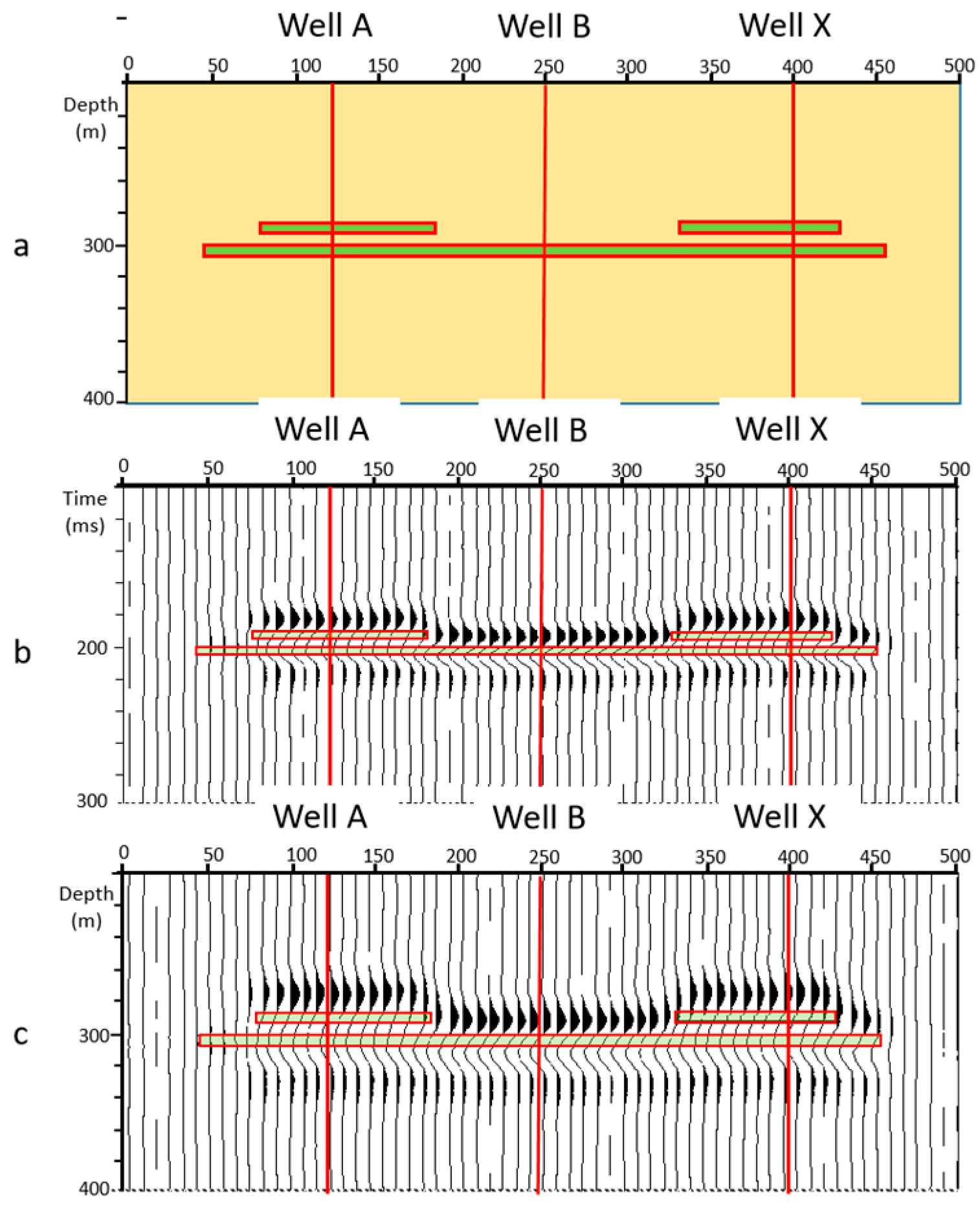
2.1. Forward Model
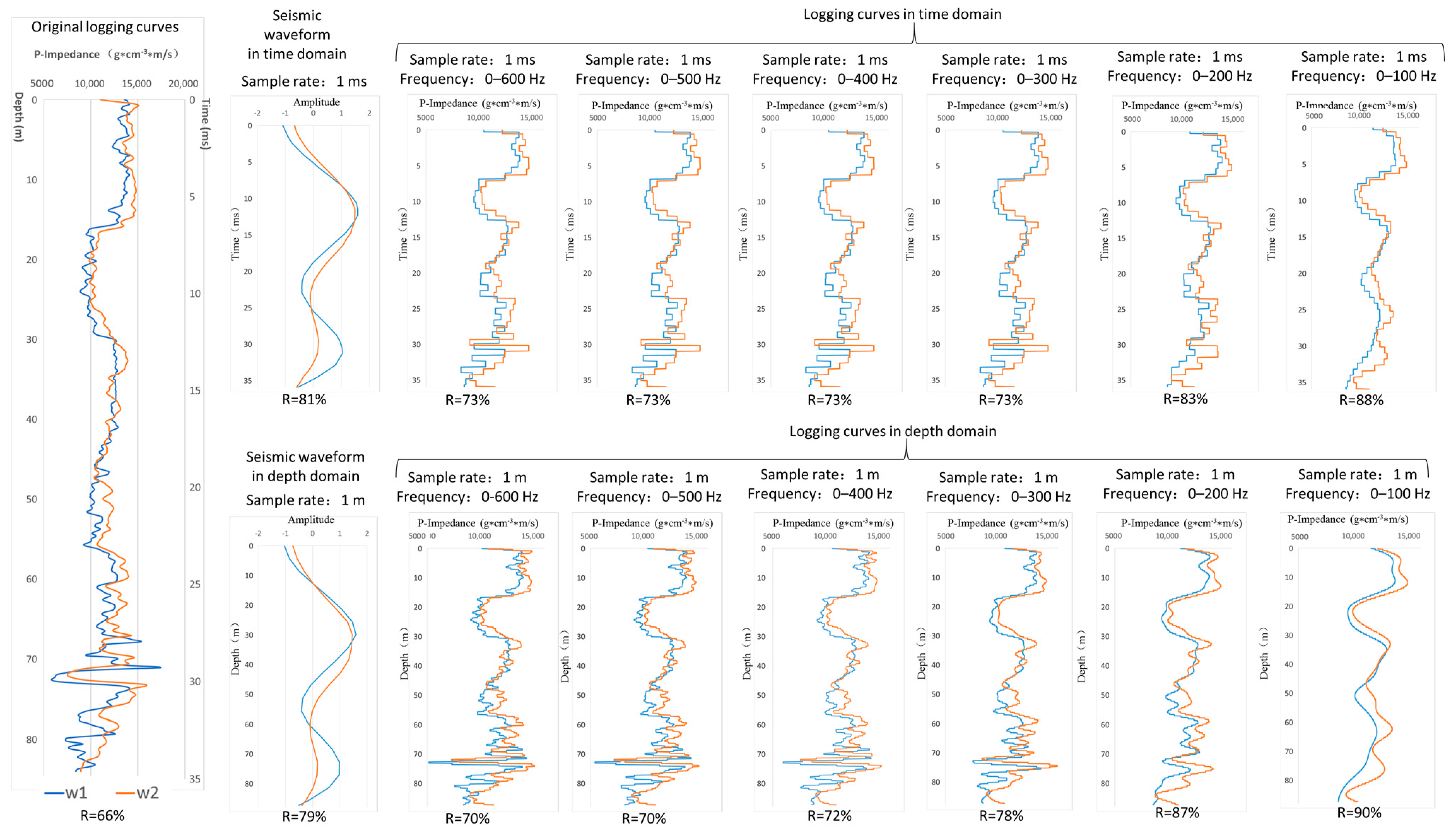
2.2. Evaluation of Depth-Domain Seismic Data
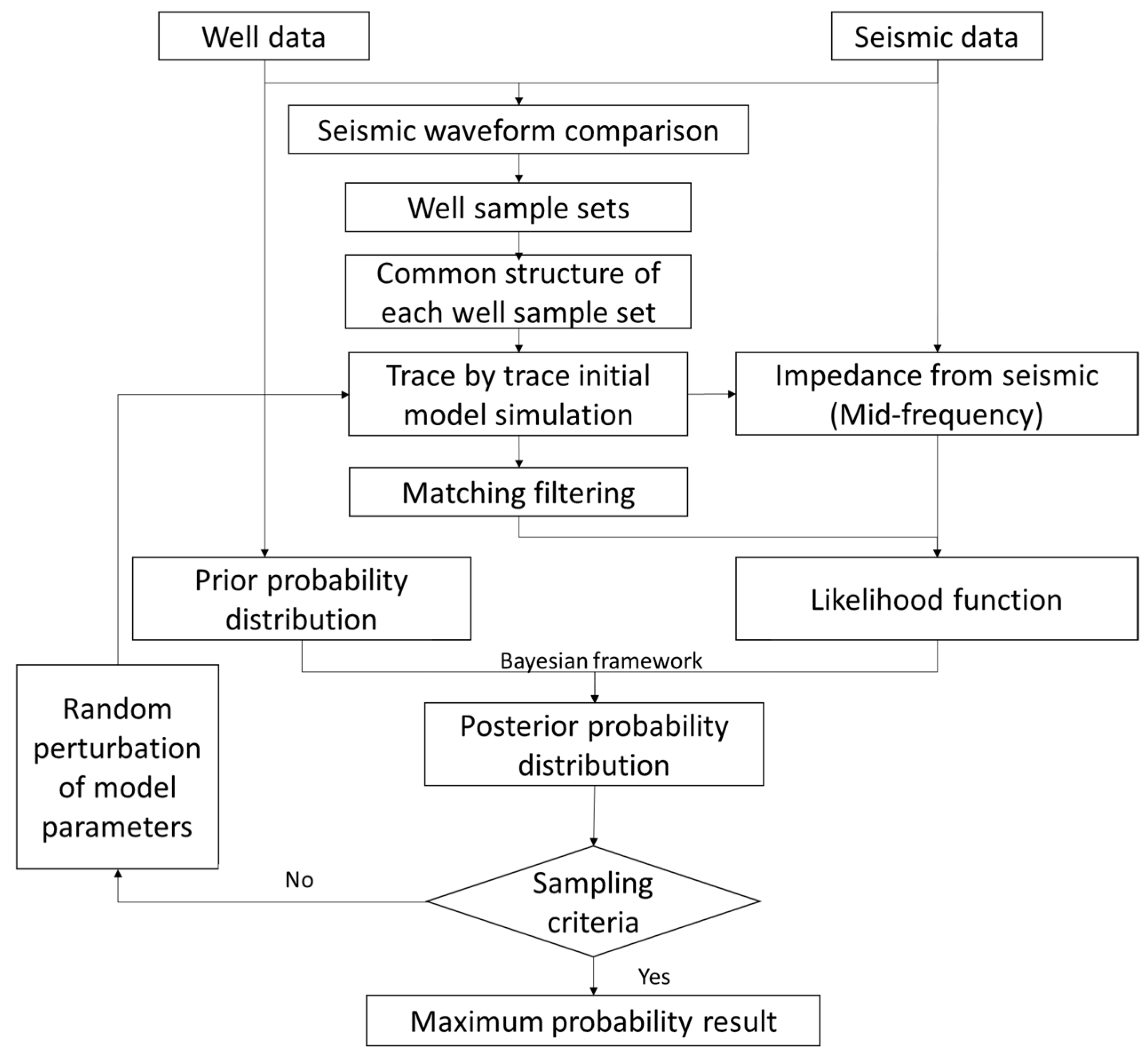
2.3. Seismic Waveform Indicator Inversion
3. Application
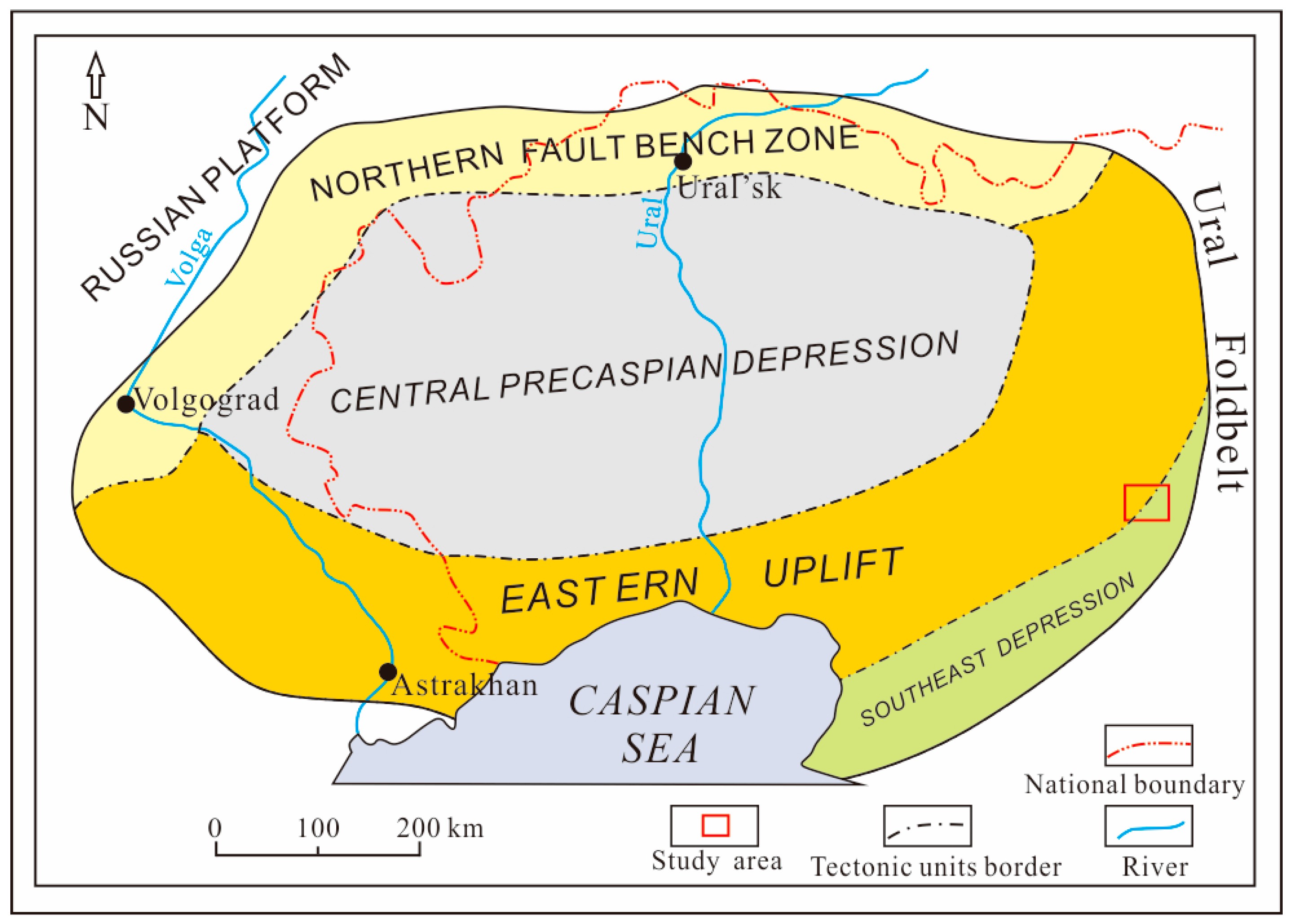
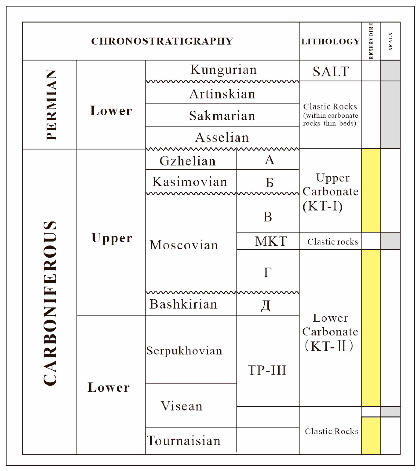
3.1. Geological Settings
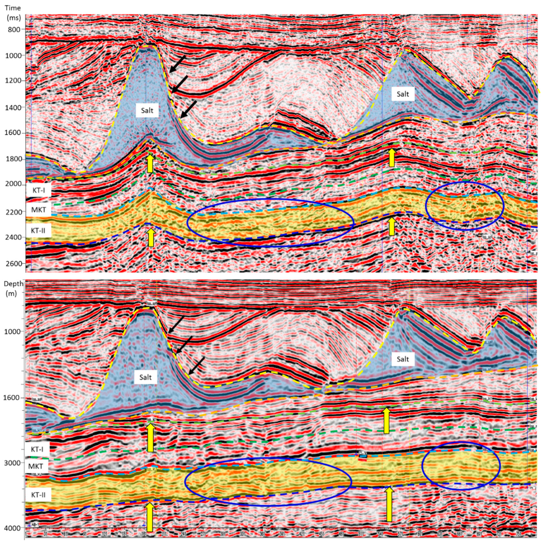
3.2. Depth Migrated Seismic Data
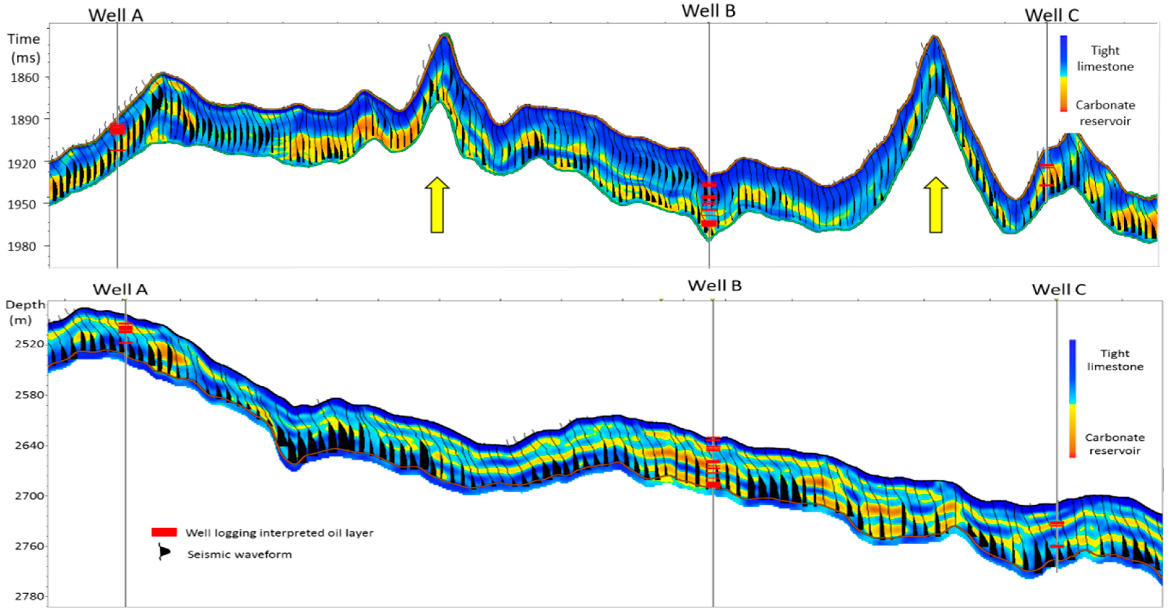
3.3. Depth Domain Seismic Inversion
4. Discussion
5. Conclusions
Author Contributions
Funding
Data Availability Statement
Acknowledgments
Conflicts of Interest
References
- Chahooki, M.Z.; Javaherian, A.; Saberi, M.R. Realization ranking of seismic geostatistical inversion based on a Bayesian lithofacies classification—A case study from an offshore field. J. Appl. Geophys. 2019, 170, 103814. [Google Scholar] [CrossRef]
- Chopra, S. Inversion in Depth? World Oil 2016, 17. Available online: https://worldoil.com (accessed on 14 March 2023).
- Macedo, I.D.; Silva, C.; Figueiredo, J.D.; Omoboya, B. Comparison between deterministic and statistical wavelet estimation methods through predictive deconvolution: Seismic to well tie example from the North Sea. J. Appl. Geophys. 2017, 136, 298–314. [Google Scholar] [CrossRef]
- He, L.; Zhao, L.; Liu, R.; Li, J.; Wang, S.; Zhao, W.; Ma, J. Complex relationship between porosity and permeability of carbonate reservoirs and its controlling factors: A case of platform facies in Pre-Caspian Basin. Pet. Explor. Dev. 2014, 41, 206–214. [Google Scholar] [CrossRef]
- Al-chalabi, M. Time-depth relationship for multi-layer depth conversion. Geophys. Prospect. 1997, 45, 471–486. [Google Scholar] [CrossRef]
- White, R.E.; O’Brien, P.N.S. Estimation of the primary seismic pulse. Geophys. Prospect. 1974, 22, 627–651. [Google Scholar] [CrossRef]
- Hu, Z.P.; Lin, B.X.; Xue, S.G. Depth domain wavelet analysis and convolution studies. Oil Geophys. Prospect. 2009, 44, 29–33. [Google Scholar]
- Fletcher, R.P.; Archer, S.; Nichols, D.; Mao, W. Inversion after depth imaging. In Proceedings of the 82nd SEG Annual International Meeting, Expanded Abstracts, Las Vegas, NV, USA, 4–9 November 2012. [Google Scholar]
- Chen, G.; Yang, W.; Liu, Y.; Wang, H.; Huang, X. Salt Structure Elastic Full Waveform Inversion Based on the Multi-scale Signed Envelope. IEEE Trans. Geosci. Remote Sens. 2022, 60, 1–12. [Google Scholar] [CrossRef]
- Chen, G.; Yang, W.; Liu, Y.; Luo, J.; Jing, H. Envelope-based sparse constrained deconvolution for velocity model building. IEEE Trans. Geosci. Remote Sens. 2022, 60, 1–13. [Google Scholar] [CrossRef]
- Singh, Y. Deterministic inversion of seismic data in the depth domain. Lead. Edge 2012, 31, 538–545. [Google Scholar] [CrossRef]
- Fletcher, R.P.; Nichols, D.; Bloor, R.; Coates, R.T. Least-squares migration-Data domain versus image domain using point spread functions. Lead. Edge 2016, 35, 157–162. [Google Scholar] [CrossRef]
- Zhang, J.L.; Xu, M.R.; Ye, Y.M. Seismogram synthetizing in the depth-domain with point spread function. Oil Geophys. Prospect. 2019, 54, 875–881. [Google Scholar]
- Zhang, R.; Zhang, K.; Alekhue, J.E. Depth-domain seismic reflectivity inversion with compressed sensing technique. Interpretation 2017, 5, T1–T9. [Google Scholar] [CrossRef]
- Zhang, R.; Deng, Z. A depth variant seismic wavelets extraction method for inversion of post-stack depth domain seismic data. Geophysics 2017, 83, R569–R579. [Google Scholar] [CrossRef]
- Sun, Y.C. Geostatistical inversion based on Bayesian-MCMC algorithm and its applications in reservoir simulation. J. Prog. Geophys. 2018, 33, 724–729. [Google Scholar] [CrossRef]
- Wang, K.Y.; Xiao, Z.J.; Jiang, Y.; Pang, S.Y.; Gao, Y.H. Seismic inversion method of stochastic stimulation in depth domain and its application. Prog. Geophys. 2017, 32, 1665–1672. (In Chinese) [Google Scholar] [CrossRef]
- Chen, X.H. Depth domain geostatistical inversion of Fuyu Group in Chaoyanggou Oilfield. Fault-Block Oil Gas Field 2018, 25, 446–449. [Google Scholar]
- Sun, S.M.; Peng, S.M. Inversion of geostatistics based on simulated annealing algorithm. Oil Geophys. Prospect. 2007, 42, 38–43. [Google Scholar]
- Gu, W.; Xu, M.; Wang, D.H.; Zheng, H.; Zhang, X.; Zhang, D.J.; Luo, J. Application of seismic motion inverison technology in thin reservoir prediction: A case study of the thin sandstone gas reservoir in the B area of Junggar Basin. Nat. Gas Geosci. 2016, 27, 2064–2069. [Google Scholar]
- Luo, H.M.; Wang, C.J.; Liu, S.H. Well-to-seismic calibration in the depth domain using dynamic depth warping. Oil Geophys. Prospect. 2018, 53, 997–1005. [Google Scholar]
- Xu, K. Hydrocarbon Accumulation Characteristics and Exploration Practices of Central Block in the Eastern Margin of the Pre-Caspian Basin; Petroleum Industry Press: Beijing, China, 2011; Volume 6, pp. 30–33. [Google Scholar]
- He, X.H. Discussion on seismic data of depth domain. Geophys. Prospect. Pet. 2004, 43, 353–358. [Google Scholar]
- Kulumbetova, G.Y.; Nursultanova, S.G.; Mailybayev, R.M. Lithological types and reservoir properties of KT-II reservoir on the eastern edge of Pre-Caspian Basin. Int. J. Eng. Res. Technol. 2019, 12, 1335–1340. [Google Scholar]
- Wang, Z.; Wang, Y.K.; Luo, M.; Ling, K.H.; Lin, Y.P. Carbonate depositional facies analysis and reservoir prediction for Central Block in Pre-Caspian Basin. Adv. Mater. Res. 2013, 73, 305–310. [Google Scholar]
- Liu, W.Q.; Wang, X.W.; Liu, H.; Wang, Y.C.; Wang, X.; Zeng, H.H.; Shao, X.C. Application of velocity modeling and reverse time migration to subsalt structure. Chinese J. Geophy. 2013, 56, 616–625. [Google Scholar]


| Correlation Coefficient of Seismic Waveforms (Time) | Frequency Bandwidth of Log Curves in Time Domain (Hz) | Correlation Coefficient of Seismic Waveforms (Depth) | Frequency Bandwidth of Log Curves in Depth Domain (Hz) |
|---|---|---|---|
| 0.81 | 0–200 | 0.79 | 0–300 |
| 0.73 | 0–200 | 0.75 | 0–300 |
| 0.68 | 0–100 | 0.64 | 0–200 |
| 0.84 | 0–200 | 0.82 | 0–300 |
| 0.77 | 0–200 | 0.77 | 0–200 |
Disclaimer/Publisher’s Note: The statements, opinions and data contained in all publications are solely those of the individual author(s) and contributor(s) and not of MDPI and/or the editor(s). MDPI and/or the editor(s) disclaim responsibility for any injury to people or property resulting from any ideas, methods, instructions or products referred to in the content. |
© 2023 by the authors. Licensee MDPI, Basel, Switzerland. This article is an open access article distributed under the terms and conditions of the Creative Commons Attribution (CC BY) license (https://creativecommons.org/licenses/by/4.0/).
Share and Cite
Hao, J.; Wu, S.; Yang, J.; Zhang, Y.; Sha, X. Application of Seismic Waveform Indicator Inversion in the Depth Domain: A Case Study of Pre-Salt Thin Carbonate Reservoir Prediction. Energies 2023, 16, 3073. https://doi.org/10.3390/en16073073
Hao J, Wu S, Yang J, Zhang Y, Sha X. Application of Seismic Waveform Indicator Inversion in the Depth Domain: A Case Study of Pre-Salt Thin Carbonate Reservoir Prediction. Energies. 2023; 16(7):3073. https://doi.org/10.3390/en16073073
Chicago/Turabian StyleHao, Jinjin, Shiguo Wu, Jinxiu Yang, Yajun Zhang, and Xuemei Sha. 2023. "Application of Seismic Waveform Indicator Inversion in the Depth Domain: A Case Study of Pre-Salt Thin Carbonate Reservoir Prediction" Energies 16, no. 7: 3073. https://doi.org/10.3390/en16073073