
Balancing the Active Power of a Railway Traction Power Substation with an sp-RPC

Abstract
:1. Introduction
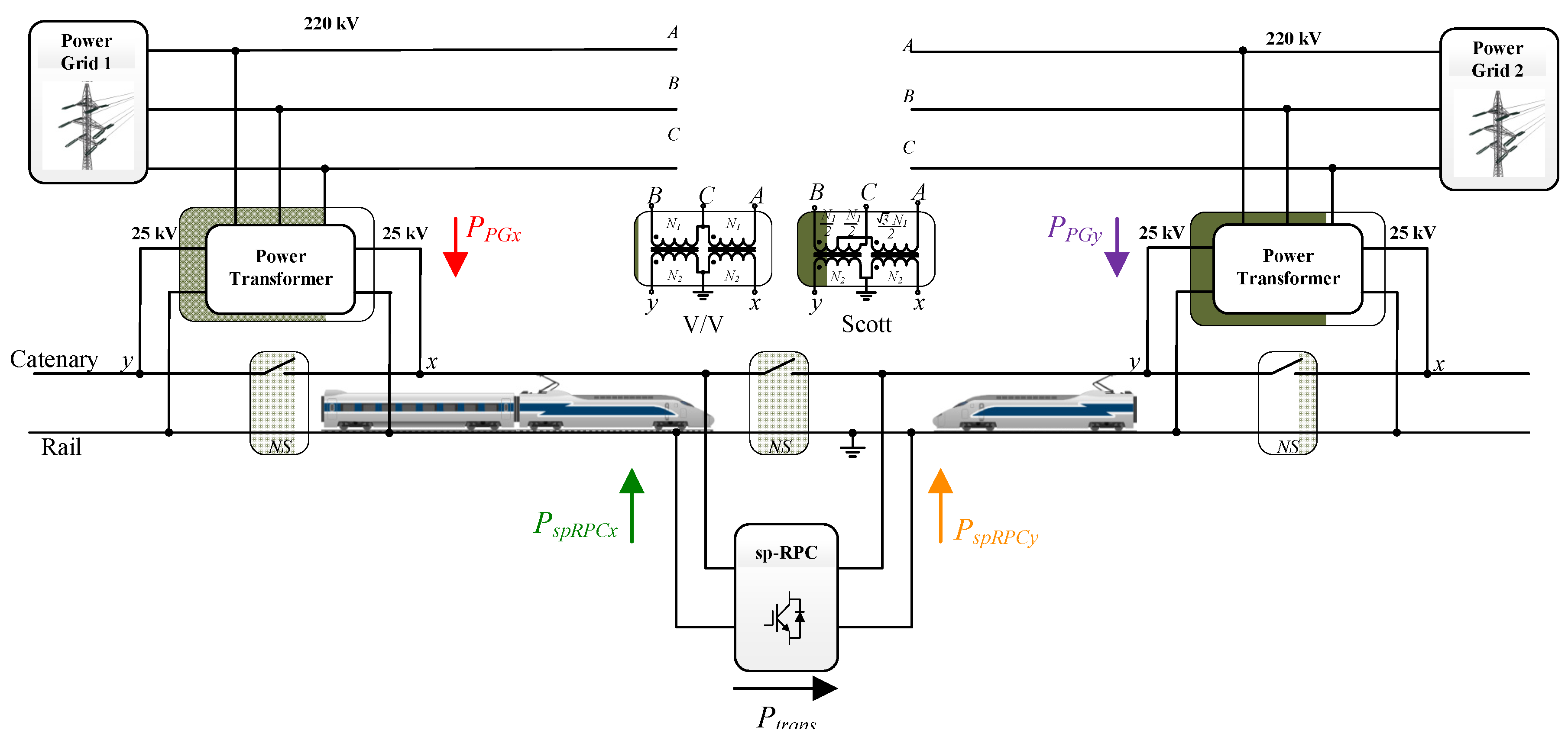
2. sp-RPC Concept
3. sp-RPC Proposed and Operation Principle
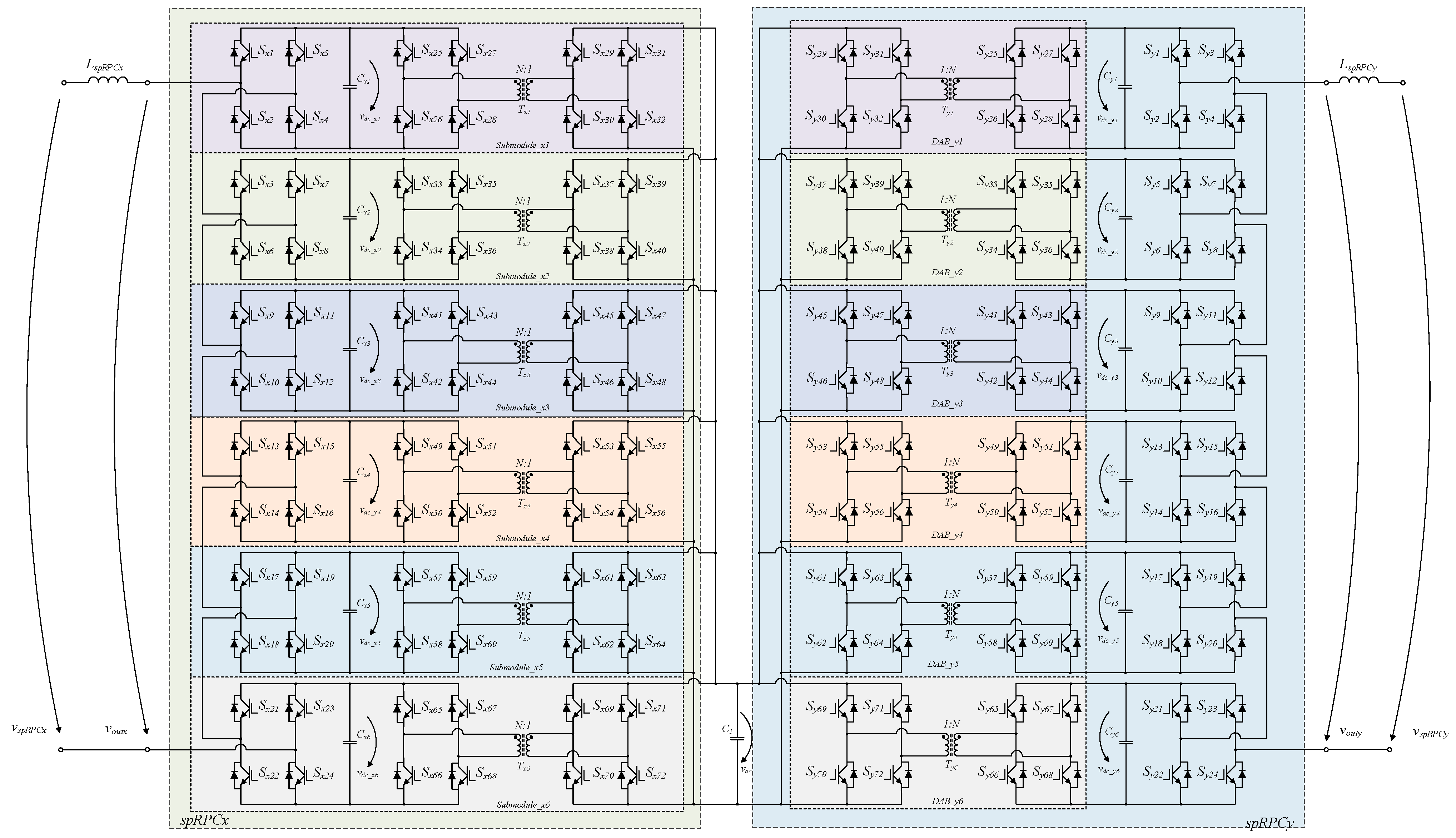
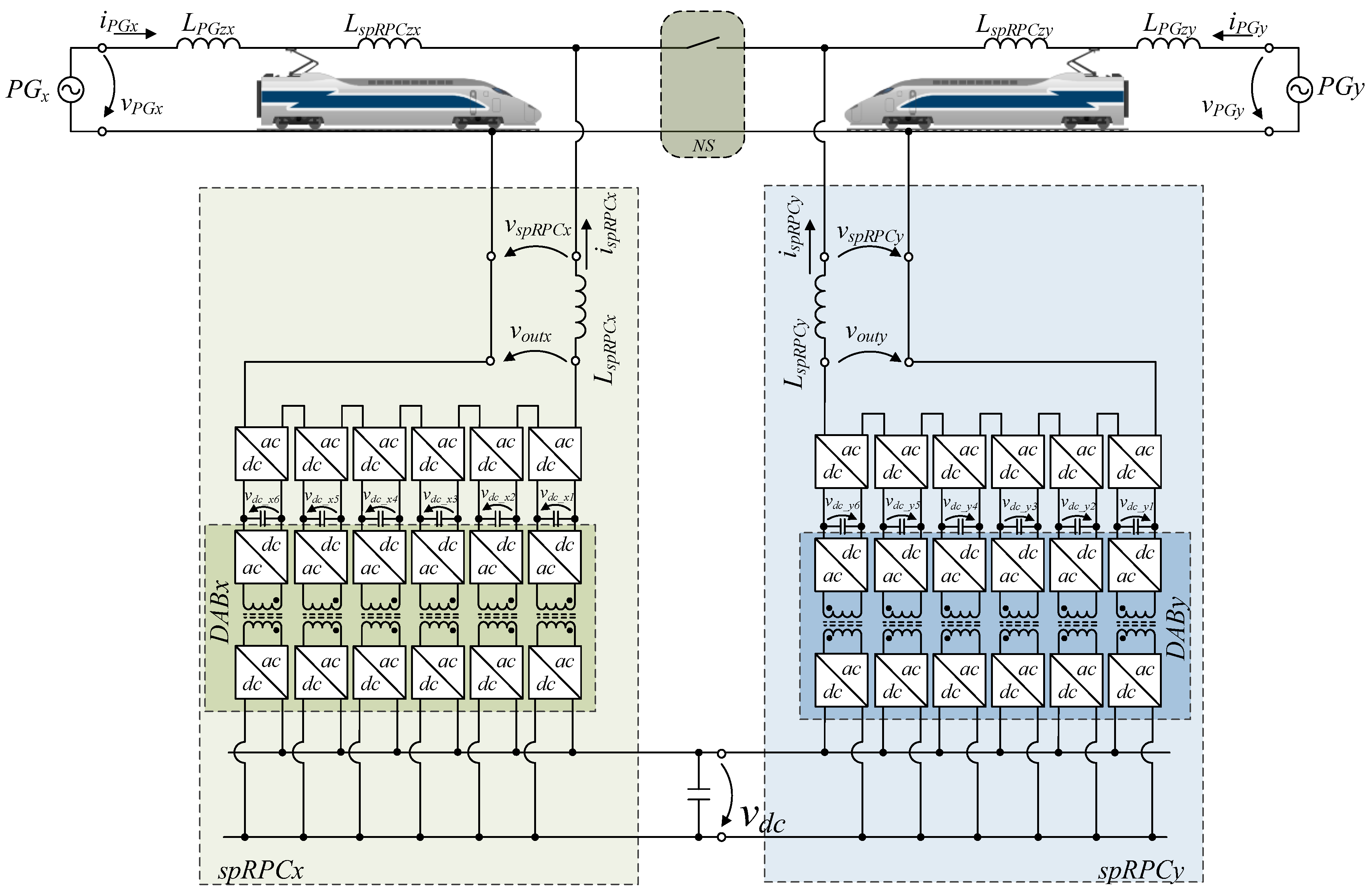
3.1. sp-RPC Topology
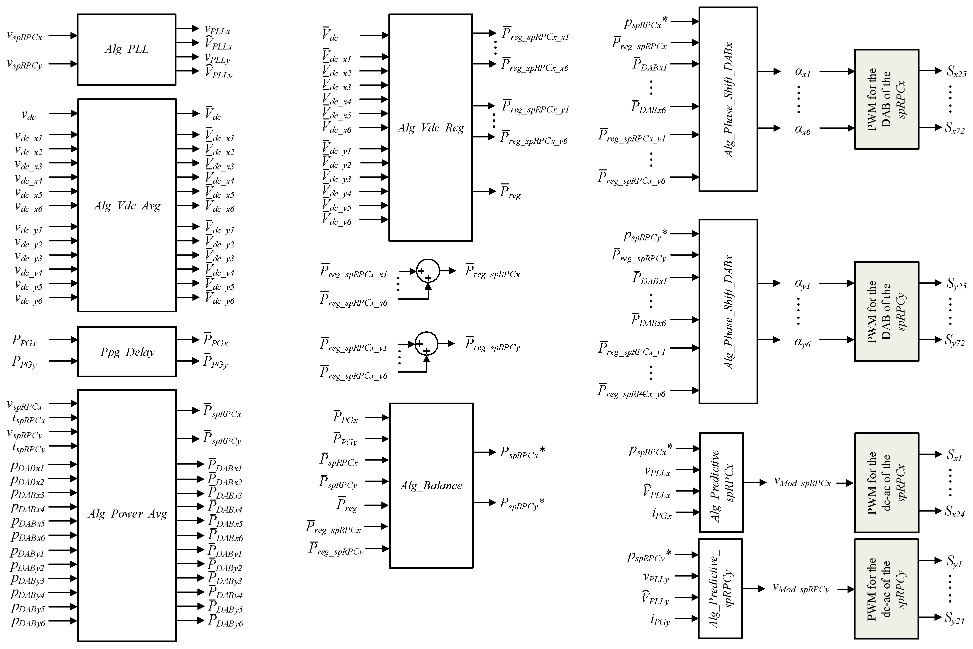
3.2. Sp-RPC Control Algorithm
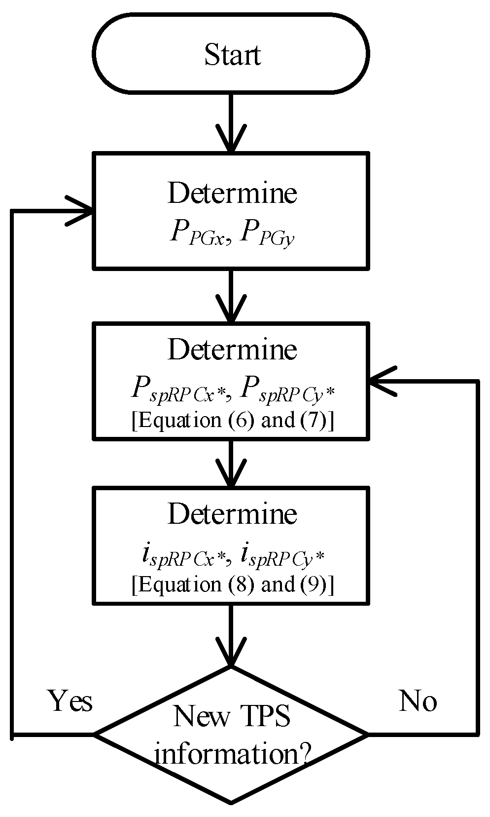
3.2.1. Dynamic sp-RPC Control
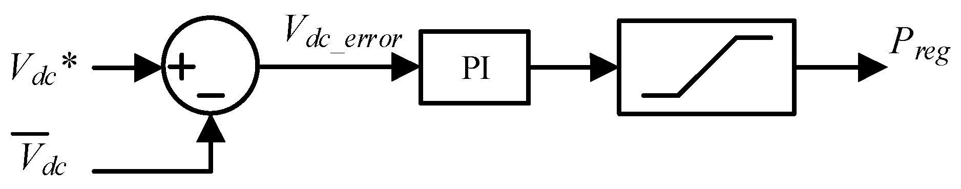
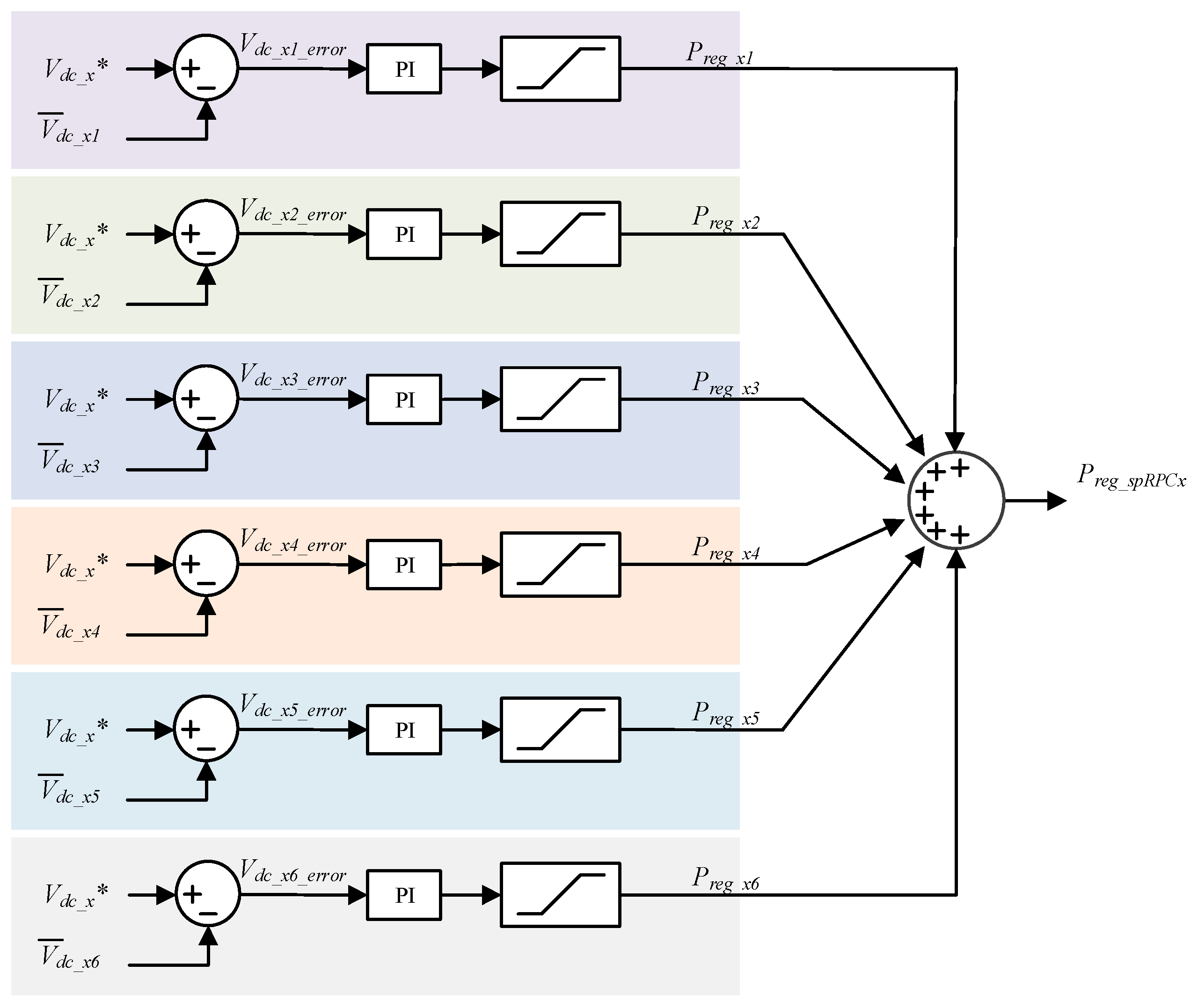
3.2.2. DC-Link Regulation
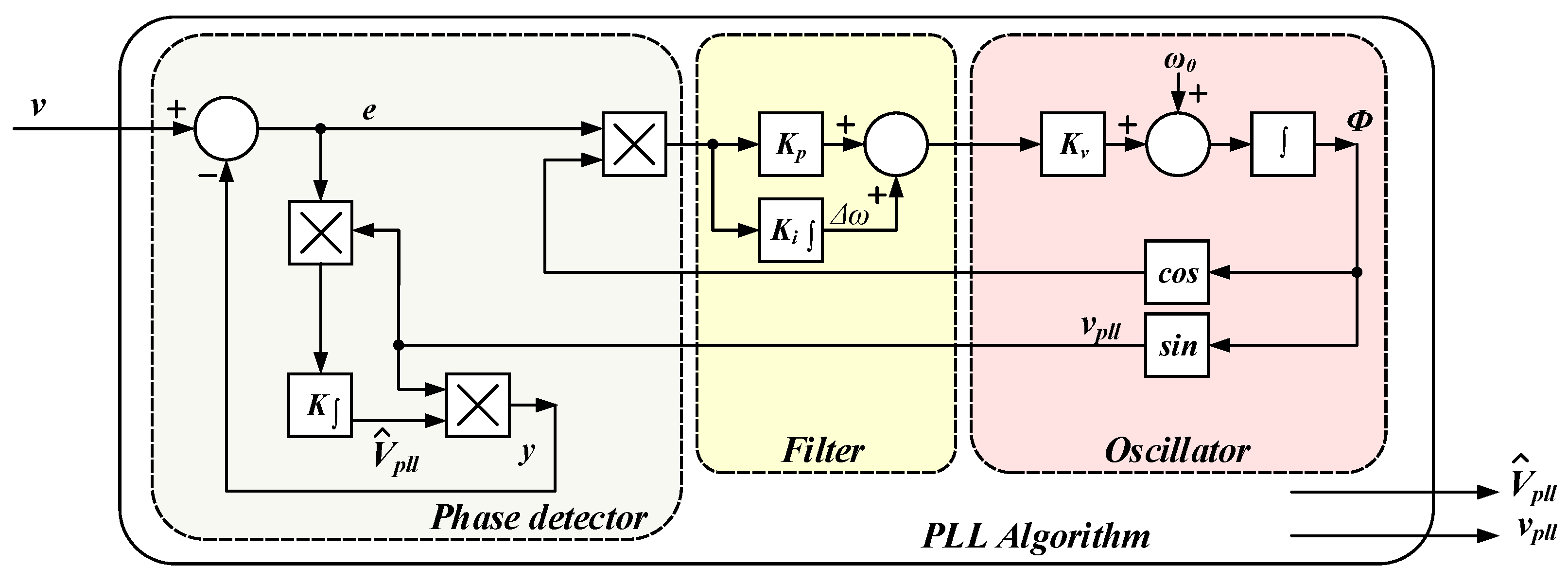
3.2.3. PLL Control Algorithm
3.2.4. Predictive Current Control Algorithm
3.2.5. PWM Techniques for Multilevel Converter
4. sp-RPC Simulation Results
4.1. Case Analysis Scenarios
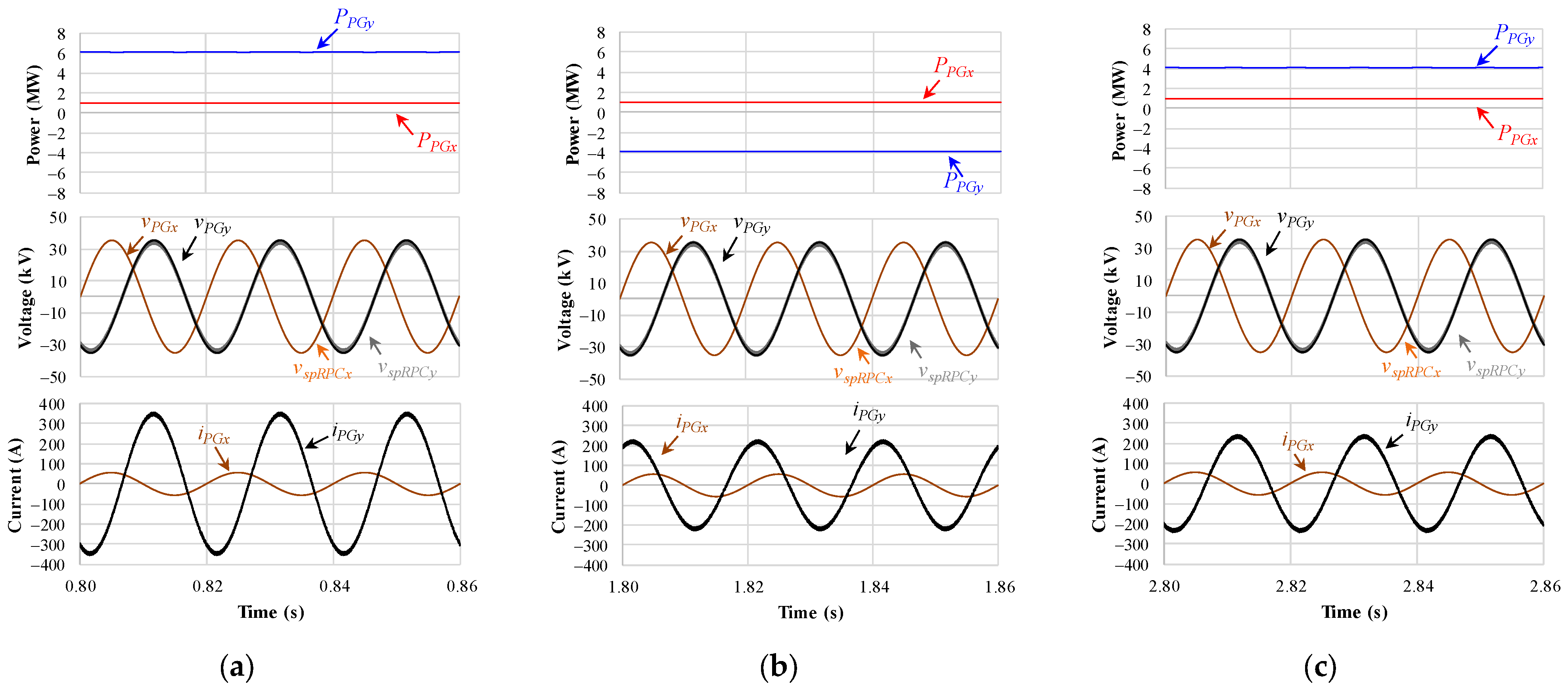
- In Figure 12a, the load on the x-side presents an average active power PLoadx = 0.998 MW, while the load on the y-side presents PLoady = 6.12 MW. Regarding the currents, it is possible to verify that iPGx presents an amplitude of 56.54 A, while iPGy presents an amplitude of 357.2 A. This case represents the event (i);
- In Figure 12b, the load on the x-side presents an average active power PLoadx = 0.998 MW, while the load on the y-side presents PLoady = −3.88 MW. Regarding the currents, it is possible to verify that iPGx presents an amplitude of 56.54 A, while iPGy presents an amplitude of 228.4 A. This case represents the event (ii);
- In Figure 12c, the load on the x-side presents an average active power PLoadx = 0.998 MW, while the load on the y-side presents PLoady = 4.12 MW. Regarding the currents, it is possible to verify that iPGx presents an amplitude of 56.54 A, while iPGy presents an amplitude of 243 A. This case represents the event (iii).
4.2. Traction Power Substation Active Power Analyses
4.3. Detailed Analysis of the sp-RPC
5. Performance Analyses of the sp-RPC
6. Discussion
7. Conclusions
Author Contributions
Funding
Data Availability Statement
Conflicts of Interest
References
- Future Population Growth. Available online: https://ourworldindata.org/future-population-growth (accessed on 24 March 2023).
- Goulding, L.; Morrell, M. Future of Rail 2050; Arup Rail: London, UK, 2019; p. 60. [Google Scholar]
- IEA—International Energy Agency. The Future of Rail: Opportunities for Energy and the Environment; IEA—International Energy Agency: Paris, France, 2019. [Google Scholar]
- UIC-ETF (Railway Technical Publications) & CER. Rail Transport and Environment: Facts & Figures; CER: Paris, France, 2015. [Google Scholar]
- CER. The Voice of European Railways: Activity Report 2019; CER: Paris, France, 2019. [Google Scholar]
- Infraestruturas de Portugal. Available online: https://www.infraestruturasdeportugal.pt/ (accessed on 30 December 2022).
- Shift2Rail Joint Undertaking. Multi-Annual Action Plan (Executive View Part A); Horizon 2020 European Union Funding for Research & Innovation: Brussels, Belgium, 2015; Available online: https://rail-research.europa.eu/wp-content/uploads/2017/11/Shift2Rail-MAAP-Part-A_Executive-View_web.pdf (accessed on 24 March 2023).
- Shift2Rail Joint Undertaking. Multi-Annual Action Plan; European Union: Brussels, Belgium, 2019; Available online: https://rail-research.europa.eu/wp-content/uploads/2020/09/MAAP-Part-A-and-B.pdf (accessed on 24 March 2023).
- Gazafrudi, S.M.M.; Langerudy, A.T.; Fuchs, E.F.; Al-Haddad, K. Power quality issues in railway electrification: A comprehensive perspective. IEEE Trans. Ind. Electron. 2015, 62, 3081–3090. [Google Scholar] [CrossRef]
- Canales, J.M.; Aizpuru, I.; Iraola, U.; Barrena, J.A.; Barrenetxea, M. Medium-Voltage AC Static Switch Solution to Feed Neutral Section in a High-Speed Railway System. Energies 2018, 11, 2740. [Google Scholar] [CrossRef] [Green Version]
- Serrano-Jiménez, D.; Abrahamsson, L.; Castaño-Solís, S.; Sanz-Feito, J. Electrical railway power supply systems: Current situation and future trends. Int. J. Electr. Power Energy Syst. 2017, 92, 181–192. [Google Scholar] [CrossRef]
- Barros, L.A.M.; Tanta, M.; Martins, A.P.; Afonso, J.L.; Pinto, J.G. STATCOM Evaluation in Electrified Railway Using V/V and Scott Power Transformers. In Proceedings of the International Conference on Sustainable Energy for Smart Cities, Braga, Portugal, 4–6 December 2019; pp. 18–32. [Google Scholar] [CrossRef]
- Li, T.; Shi, Y. Application of MMC-RPC in High-Speed Railway Traction Power Supply System Based on Energy Storage. Appl. Sci. 2022, 12, 10009. [Google Scholar] [CrossRef]
- Song, S.; Liu, J.; Ouyang, S.; Chen, X. A modular Multilevel Converter Based Railway Power Conditioner for Power Balance and Harmonic Compensation in Scott Railway Traction System. In Proceedings of the 2016 IEEE 8th International Power Electronics and Motion Control Conference (IPEMC-ECCE Asia), Hefei, China, 22–26 May 2016; pp. 2412–2416. [Google Scholar] [CrossRef]
- Li, T.; Shi, Y. Power Quality Management Strategy for High-Speed Railway Traction Power Supply System Based on MMC-RPC. Energies 2022, 15, 5205. [Google Scholar] [CrossRef]
- Tanta, M.; Cunha, J.; Barros, L.A.; Monteiro, V.; Pinto, J.; Martins, A.P.; Afonso, J.L. Experimental Validation of a Reduced-Scale Rail Power Conditioner Based on Modular Multilevel Converter for AC Railway Power Grids. Energies 2021, 14, 484. [Google Scholar] [CrossRef]
- Barros, L.A.M.; Tanta, M.; Martins, A.P.; Afonso, J.L.; Pinto, J.G. Opportunities and Challenges of Power Electronics Systems in Future Railway Electrification. In Proceedings of the 2020 IEEE 14th International Conference on Compatibility, Power Electronics and Power Engineering (CPE-POWERENG), Setubal, Portugal, 8–10 July 2020. [Google Scholar] [CrossRef]
- Aoki, K.; Kikuchi, K.; Seya, M.; Kato, T. Power Interchange System for Reuse of Regenerative Electric Power. Hitachi Rev. 2015, 67, 834–835. [Google Scholar]
- Morais, V.A.; Martins, A.P. Traction power substation balance and losses estimation in AC railways using a power transfer device through Monte Carlo analysis. Railw. Eng. Sci. 2022, 30, 71–95. [Google Scholar] [CrossRef]
- Kosugi, R.; Ji, S.; Mochizuki, K.; Adachi, K.; Segawa, S.; Kawada, Y.; Yonezawa, Y.; Okumura, H. Breaking the Theoretical Limit of 6.5 kV-Class 4H-SiC Super-Junction (SJ) MOSFETs by Trench-Filling Epitaxial Growth. In Proceedings of the 2019 31st International Symposium on Power Semiconductor Devices and ICs (ISPSD), Shanghai, China, 19–23 May 2019; pp. 39–42. [Google Scholar] [CrossRef]
- Kadavelugu, A.; Bhattacharya, S.; Ryu, S.-H.; Van Brunt, E.; Grider, D.; Agarwal, A.; Leslie, S. Characterization of 15 kV SiC n-IGBT and its application considerations for high power converters. In Proceedings of the 2013 IEEE energy conversion congress and exposition, Denver, CO, USA, 15–19 September 2013; pp. 2528–2535. [Google Scholar] [CrossRef] [Green Version]
- Howell, R.S.; Buchoff, S.; Van Campen, S.; McNutt, T.R.; Ezis, A.; Nechay, B.; Kirby, C.F.; Sherwin, M.E.; Clarke, R.C.; Singh, R. A 10-kV Large-Area 4H-SiC Power DMOSFET with Stable Subthreshold Behavior Independent of Temperature. IEEE Trans. Electron Devices 2008, 55, 1807–1815. [Google Scholar] [CrossRef]
- Passmore, B.; Cole, Z.; McGee, B.; Wells, M.; Stabach, J.; Bradshaw, J.; Shaw, R.; Martin, D.; McNutt, T.; VanBrunt, E.; et al. The next generation of high-voltage (10 kV) silicon carbide power modules. In Proceedings of the 2016 IEEE 4th Workshop on Wide Bandgap Power Devices and Applications (WiPDA), Fayetteville, AR, USA, 7–9 November 2016; pp. 1–4. [Google Scholar] [CrossRef]
- Das, M.K.; Capell, C.; Grider, D.E.; Leslie, S.; Ostop, J.; Raju, R.; Schutten, M.; Nasadoski, J.; Hefner, A. 10 kV, 120 A SiC half H-bridge power MOSFET modules suitable for high frequency, medium voltage applications. In Proceedings of the 2011 IEEE Energy Conversion Congress and Exposition, Phoenix, AZ, USA, 17–22 September 2011; pp. 2689–2692. [Google Scholar] [CrossRef]
- Barros, L.A.M.; Martins, A.P.; Pinto, J.G. A Comprehensive Review on Modular Multilevel Converters, Submodule Topologies, and Modulation Techniques. Energies 2022, 15, 1078. [Google Scholar] [CrossRef]
- Pinto, J.G.; Monteiro, V.; Goncalves, H.; Afonso, J.L. Onboard reconfigurable battery charger for electric vehicles with traction-to-auxiliary mode. IEEE Trans. Veh. Technol. 2013, 63, 1104–1116. [Google Scholar] [CrossRef] [Green Version]
- Gohil, G.; Wang, H.; Liserre, M.; Kerekes, T.; Teodorescu, R.; Blaabjerg, F. Reduction of DC-link capacitor in case of cascade multilevel converters by means of reactive power control. In Proceedings of the 2014 IEEE Applied Power Electronics Conference and Exposition-APEC, Fort Worth, TX, USA, 16–20 March 2014; pp. 231–238. [Google Scholar] [CrossRef] [Green Version]
- Karimi-Ghartemani, M.; Iravani, M.R. A Method for synchronization of power electronic converters in polluted and variable-frequency environments. IEEE Trans. Power Syst. 2004, 19, 1263–1270. [Google Scholar] [CrossRef]
- Karimi-Ghartemani, M. Enhanced Phase-Locked Loop Structures for Power and Energy Applications; John Wiley & Sons: Hoboken, NJ, USA, 2014. [Google Scholar] [CrossRef]
- Blaabjerg, F.; Teodorescu, R.; Liserre, M.; Timbus, A.V. Overview of control and grid synchronization for distributed power generation systems. IEEE Trans. Ind. Electron. 2006, 53, 1398–1409. [Google Scholar] [CrossRef] [Green Version]
- Monteiro, V.; Oliveira, C.F.; Afonso, J.L. Experimental Validation of a Bidirectional Multilevel dc-dc Power Converter for Electric Vehicle Battery Charging Operating under Normal and Fault Conditions. Electronics 2023, 12, 851. [Google Scholar] [CrossRef]
- Basri, H.M.; Lias, K. Predictive Current Control of Three Level Neutral Point Clamped Based Indirect Matrix Converter. In Proceedings of the 2019 International UNIMAS STEM 12th Engineering Conference (EnCon), Kuching, Malaysia, 28–29 August 2019; pp. 16–21. [Google Scholar] [CrossRef] [Green Version]


| Variable | Nominal | Unit | |
|---|---|---|---|
| Nominal active power for the sp-RPC | Psp_RPCx, Psp_RPCy | 2.5 | MW |
| Common dc-Link nominal voltage | Vdc | 1 | kV |
| Nominal voltage on the dedicated dc-links of the sp-RPC | Vdc_x1, Vdc_x2, Vdc_x3, Vdc_x4, Vdc_x5, Vdc_x6, Vdc_y1, Vdc_y2, Vdc_y3, Vdc_y4, Vdc_y5, Vdc_y6 | 7 | kV |
| Catenary nominal voltage | vPGx, vPGy | 25 | kV |
| sp-RPC output nominal current | ispRPCx, ispRPCy | 100 | A |
| Communication frequency between TPS and the sp-RPC | fs_PG | 5 | Hz |
| Sampling frequency for the sp-RPC | fs | 50 | kHz |
| Switching frequency for the ac side | fsw_spRPC | 1 | kHz |
| Switching frequency for the DAB | fsw_spRPC_DAB | 1 | kHz |
| Variable | Value | Unit | |
|---|---|---|---|
| Line impedance inductors | LPGzx, LPGzy, LspRPCzx, LspRPCzx, | 2.5 (250 #1) | mH (mΩ) |
| Coupling inductor | LspRPCx, LspRPCy | 50 (10 #1) | mH (mΩ) |
| Capacitance on the dc-link | C1 | 200 (10 #1) | mF (mΩ) |
| Capacitance on the dc-link | Cx1, Cx2, Cx3, Cx4, Cx5, Cx6, Cy1, Cy2, Cy3, Cy4, Cy5, Cy6 | 10 (10 #1) | mF (mΩ) |
| sp-RPC Disabled | sp-RPC Enabled | |||||||
|---|---|---|---|---|---|---|---|---|
| Event | (i) | (ii) | (iii) | (i) | (ii) | (iii) | ||
| Parameters | ||||||||
| iPGx | 39.97 | 39.97 | 39.97 | 144 | 56.9 | 102 | A | |
| iPGy | 245.8 | 155 | 165.4 | 143 | 63.5 | 104 | A | |
| ispRPCx | - | - | - | 105 | 97 | 62.4 | A | |
| ispRPCy | - | - | - | 100 | 100 | 61.4 | A | |
| vPGx | 24,992 | 24,992 | 24,994 | 24,983 | 25,004 | 24,987 | V | |
| vPGy | 24,982 | 25,018 | 24,985 | 24,990 | 25,005 | 24,992 | V | |
| vspRPCx | 24,982 | 24,982 | 24,984 | 24,923 | 25,043 | 24,950 | V | |
| vspRPCy | 24,940 | 25,081 | 24,968 | 25,013 | 25,014 | 25,000 | V | |
| PLoadx | 999 | 999 | 999 | 999 | 999 | 999 | kW | |
| PLoady | 6119 | −3884 | 4122 | 6119 | −3884 | 4122 | kW | |
| PPGx | 999 | 999 | 999 | 3612 | −1419 | 2565 | kW | |
| PPGy | 6119 | −3884 | 4122 | 3626 | −1367 | 2565 | kW | |
| PspRPCx | - | - | - | −2608 | 2424 | −1564 | kW | |
| PspRPCy | - | - | - | 2507 | 2507 | 1534 | kW | |
| PPG_off | 3559 | −1442 | 2560 | - | - | - | kW | |
| PPG_on | - | - | - | 3619 | −1393 | 2565 | kW | |
| PPG_%inc | - | - | - | 1.7 | −3.4 | 0.2 | % | |
| Unbalance | 71.9 | 169.3 | 61.0 | 0.19 | 1.86 | 0 | % | |
Disclaimer/Publisher’s Note: The statements, opinions and data contained in all publications are solely those of the individual author(s) and contributor(s) and not of MDPI and/or the editor(s). MDPI and/or the editor(s) disclaim responsibility for any injury to people or property resulting from any ideas, methods, instructions or products referred to in the content. |
© 2023 by the authors. Licensee MDPI, Basel, Switzerland. This article is an open access article distributed under the terms and conditions of the Creative Commons Attribution (CC BY) license (https://creativecommons.org/licenses/by/4.0/).
Share and Cite
Barros, L.A.M.; Martins, A.P.; Pinto, J.G. Balancing the Active Power of a Railway Traction Power Substation with an sp-RPC. Energies 2023, 16, 3074. https://doi.org/10.3390/en16073074
Barros LAM, Martins AP, Pinto JG. Balancing the Active Power of a Railway Traction Power Substation with an sp-RPC. Energies. 2023; 16(7):3074. https://doi.org/10.3390/en16073074
Chicago/Turabian StyleBarros, Luis A. M., António P. Martins, and José Gabriel Pinto. 2023. "Balancing the Active Power of a Railway Traction Power Substation with an sp-RPC" Energies 16, no. 7: 3074. https://doi.org/10.3390/en16073074