Research on Data-Driven Optimal Scheduling of Power System

Abstract

The uncertainty of output makes it difficult to effectively solve the economic security dispatching problem of the power grid when a high proportion of renewable energy generating units are integrated into the power grid. Based on the proximal policy optimization (PPO) algorithm, a safe and economical grid scheduling method is designed. First, constraints on the safe and economical operation of renewable energy power systems are defined. Then, the quintuple of Markov decision process is defined under the framework of deep reinforcement learning, and the dispatching optimization problem is transformed into Markov decision process. To solve the problem of low sample data utilization in online reinforcement learning strategies, a PPO optimization algorithm based on the Kullback–Leibler (KL) divergence penalty factor and importance sampling technique is proposed, which transforms on-policy into off-policy and improves sample utilization. Finally, the simulation analysis of the example shows that in a power system with a high proportion of renewable energy generating units connected to the grid, the proposed scheduling strategy can meet the load demand under different load trends. In the dispatch cycle with different renewable energy generation rates, renewable energy can be absorbed to the maximum extent to ensure the safe and economic operation of the grid.

1. Introduction

The fluctuation and intermittent behavior of wind power and other renewable energies are highly uncertain, and their impact on electric power reliability, power quality and economy is increasingly prominent with the increase in permeability [1,2]. With the large-scale grid connection of renewable energy, the uncertainty of power system operation increases significantly [3]. The optimal dispatching of power network also changes from deterministic optimization to uncertainty optimization [4]. Stochastic optimization and robust optimization are two common methods for the uncertainty optimization of power systems. Stochastic optimization requires the construction of probabilistic models of random variables [5,6]. Refs. [7,8] respectively consider wind speed and solar irradiance as random variables subject to Weibull distribution and beta distribution, and use random variables to describe the uncertainty of wind power and photovoltaic output. Weibull distribution is a continuous probability distribution. Beta distribution is a density function as a prior conjugate distribution of Bernoulli and binomial distributions. However, the current output of wind power, photovoltaic and other renewable energy units is characterized by randomness, intermittency and volatility. In addition, the load itself is also random. For the system containing complex random factors, it is more difficult to accurately model the overall randomness. The robust optimization uses the uncertainty set to describe the range of uncertainty factors. Although it does not need to set the probability distribution of random variables, the scheduling result may be conservative because the optimal solution under the worst state is considered [9].

With the improvement of the power grid measurement system and the development of renewable energy, massive renewable energy power generation data were accumulated. In order to overcome the shortcomings of traditional stochastic optimization and robust optimization in practical applications, many data-driven optimization scheduling methods have emerged [10]. These data-driven optimal scheduling methods can be divided into two categories:

• A random variable model is established based on the history or forecast data of renewable energy generation to improve the applicability of scheduling scheme in actual system operation;
• To explore the statistical information represented by data, data-driven distributionally robust optimization (DRO) has been studied to solve the problem of the inaccurate modeling of uncertainty factors in traditional stochastic optimization and to reduce the conservatism of traditional robust optimization [11,12].

However, in recent years, the proportion of renewable energy generation equipment connected to the grid has been increasing. Its randomness and discontinuity greatly increase the difficulty of solving traditional scheduling optimization methods. Deep reinforcement learning will study depth perception combined with reinforcement learning decision-making ability. It has broad prospects in application in power system dispatching [13]. The potential features of historical data are mined through deep learning, and the direction of decision is learned from the environment based on repeated adjustments of rewards and actions until the optimal goal is achieved. Reinforcement learning uses massive renewable energy generation data to interact with the power system environment to obtain a large number of scheduling data. Deeper connections between data can be mined to figure out the problem of the complexity of power system modeling and the optimal scheduling of a complex system under an uncertain environment [14]. In literature [15], the valve point effect is considered in unit cost function, and a multi-agent fuzzy reinforcement learning algorithm is applied to solve economic scheduling problems at a single time. Literature [16] takes into account the fact that the unit cost coefficient is difficult to obtain accurately in actual power networks, and uses the distributed reinforcement learning algorithm to solve unit combination and economic scheduling problems. The above works give full play to the advantage that reinforcement learning does not require precise expression of optimization objectives and environment, but they all focus on economic scheduling at a single moment, so they ignore unit climbing constraints and fail to consider the impact of subsequent environmental uncertainties on the current scheduling scheme. In literature [17], a multi-agent deep reinforcement learning algorithm with strategic goals of the real-time optimal scheduling of the active distribution system is proposed, in which the uncertainty of renewable generation, loads and electricity prices are considered to achieve real-time optimal scheduling of the active distribution system. Literature [18] focuses on the problem that existing scheduling methods cannot accurately deal with the dynamic changes in the supply-demand side of power-gas-heat IES due to power uncertainty. An optimal scheduling framework based on the asynchronous advantage law-critic (A3C) method of IES is proposed. The training time is shortened, and the daily operation cost is reduced. However, the scheduling objectives of the above works only consider the lowest operating cost, which belongs to the single objective scheduling model and does not consider the issue of available energy absorption.

In view of the above deficiencies, this paper comprehensively considers the safety, economy and renewable energy consumption rate of the power grid. The historical operation data of the power grid are preprocessed, the dispatching model of economic security operation is established, and the dispatching optimization problem is normalized as a Markov decision problem. State space, action space, and reward function are defined. The optimization of the objective function is transformed into the optimization of the reinforcement learning reward function, and the uncertainty of long-term dispatching is fully considered. A proximal policy optimization algorithm with the KL divergence penalty factor and important sampling technique is proposed to optimize the reward function of reinforcement learning. The important sampling technique is used to transform the on-policy into the off-policy, which greatly improves the utilization rate of training samples. The KL divergence penalty factor is used to determine the degree of difference between old and new strategies in the update process to improve the stability of policy updates.

In order to cope with the influence of a high proportion of renewable energy on the power system, this paper designs an economical and safe operation scheduling method based on the PPO algorithm. The main research includes defining the scheduling model of the renewable energy power system, setting the objective function and constraint conditions. Based on the deep reinforcement learning framework, the action space, state space, penalty value, and immediate reward are defined. The PPO algorithm of the KL divergence penalty factor and important sampling technique are introduced. Finally, the adaptability and effectiveness of the proposed method are verified by simulation.

2. The Power System Scheduling Model with Renewable Energy

2.1. Objective Function

Taking into account the safety of grid operation, renewable consumption efficiency and operating cost, the minimum objective function F is achieved in a scheduling cycle:

$$F={\omega }_{cost}{F}_{cost,t}-{\omega }_{con}{F}_{con,t}-{\omega }_{lim}{F}_{lim,t}$$

(1)

where ${\omega }_{cost}$, ${\omega }_{con}$ and ${\omega }_{lim}$ are the weighting coefficients of the unit operating cost function, renewable energy consumption function and line overlimit function, respectively.

• Unit operating cost function:

  $$F_{cost,t}=\sum _{i=1}^N(a_i{P}_{i,t}^2+b_i{P}_{i,t}+c_i)+C_{on,off}$$

  (2)

  where N is the total number of units; $P_{i,t}$ is the active power output of the unit i in the scheduling period t; $a_i$, $b_i$, $c_i$ is the power generation cost coefficient of unit i; $C_{on,off}$ is the unit start-stop cost. The unit start-stop cost is determined according to whether the unit’s active power output is zero.
• Renewable energy consumption function:

  $$F_{con,t}=\sum _{i=1}^{N_{re}}{P}_{i,t}/\sum _{i=1}^{N_{re}}\overline{P_{i,t}}$$

  (3)

  where $N_{re}$ is the total number of renewable energy units, $P_{i,t}$ is the active power output of the I-th renewable energy unit in the scheduling period t, and $\overline{P_{i,t}}$ is the maximum active power output of the I-th renewable energy unit in the scheduling period t.
• Line overlimit function:

  $$F_{lim,t}=1-\frac{1}{N_{line}}\sum _{i=1}^{N_{line}}min(\frac{I_{i,t}}{I_{i,max}+\in },1)$$

  (4)

  where $N_{line}$ is the number of branches of the power network; $I_{i,t}$ is the current through the i branch at time t; $I_{i,max}$ is the maximum current allowed through the line i; and ∈ is a constant of 0.001 to prevent the denominator from being 0.

2.2. Constraint Condition

• Power balance constraints:
  At any given time, the total active power of thermal power units, renewable energy units and balancing units shall be equal to the total active power of the load:

  $$\sum _{i=1}^{n_{con}}{P}_{con,i,t}+\sum _{i=1}^{n_{th}}{P}_{th,i,t}+P_{bal,t}-\sum _{i=1}^{n_{load}}{P}_{load,i,t}=0$$

  (5)

  where $n_{con}$, $n_{th}$, and $n_{load}$ refer to the number of renewable energy units, thermal power units and load, respectively. $P_{con,i,t}$ is the active power output of the i renewable energy unit at time t; $P_{th,i,t}$ is the active power output of the i thermal power unit at time t; $P_{bal,t}$ is the active power output of the balancing unit at time t; and $P_{load,i,t}$ is the active power consumed by the i load at time t.
• Unit output upper and lower limits constraints:
  At any given time, the active power output of any unit shall not be greater than the upper limit of the active power output, nor less than the lower limit of the active power output:

  $$P_{th,i,min}\le P_{th,i,t}\le P_{th,i,max}$$

  (6)

  where $P_{th,i,min}$ and $P_{th,i,max}$ are the minimum and maximum active output of the i thermal power unit, respectively:

  $$0\le P_{con,i,t}\le P_{con,i,max}$$

  (7)

  where $P_{con,i,max}$ is the maximum active output of the i renewable energy unit.
  The balance unit is used to share the system power imbalance caused by unreasonable scheduling policies and power flow calculation; the maximum output of the balance unit cannot exceed the upper limit of 110%, and the minimum cannot be lower than the lower limit of 90%:

  $$0.9P_{bal,min}\le P_{bal,t}\le 1.1P_{bal,max}$$

  (8)

  where $P_{bal,min}$ and $P_{bal,max}$ are the minimum and maximum active output of the balancing unit, respectively.
• Climbing constraint of thermal power unit:
  The output adjustment values of any thermal power unit should meet the climbing constraint:

  $$D_{th,i}\le P_{th,i,t+1}\le U_{th,i}$$

  (9)

  $$D_{th,i}=max((P_{th,i,min}-P_{th,i,t}),-rate\ast P_{th,i,max})$$

  (10)

  $$U_{th,i}=min((P_{th,i,max}-P_{th,i,t}),rate\ast P_{th,i,max})$$

  (11)

  where rate is the climbing rate of the thermal power unit; $P_{th,i,min}-P_{th,i,t}$ is the maximum value that the thermal power unit can actually adjust downwards at time t + 1; and $-rate\ast P_{th,i,max}$ is the maximum downclimb constraint value. The maximum value $D_{th,i}$ of the two values is the maximum downclimb value allowed to be adjusted by the unit i. $P_{th,i,max}-P_{th,i,t}$ is the maximum value that the thermal power unit can actually adjust upwards at time t + 1, and $-rate\ast P_{th,i,max}$ is the maximum upward-climb constraint value. The minimum value $U_{th,i}$ of the two values is the maximum climbing value allowed to be adjusted by the unit i.

3. Data-Driven Reinforcement Learning Scheduling Algorithm

3.1. Deep Reinforcement Learning Framework

The reinforcement learning process can be described by the Markov decision process (MDP), which is generally represented by a quintuple (S, A, P, R, $\gamma$), where S is the state space, A is the action space, P is the state transition probability, R is the reward function, and $\gamma$ is the discount factor [19].

The choice of the state space should be the factor influencing the decision. Combined with the research content of this paper.The state space includes the active power output of thermal power units ($P_{th,t}$), the active power output of renewable energy units ($P_{con,t}$) and the active power output of balancing units at the current time ($P_{bal,t}$). We have the branch current load rate ($rh{o}_t$), load demand at the next moment ($P_{d,t+1}$), and maximum output of the renewable energy unit at the current moment ($P_{th,max,t}$):

$$S_t=\{P_{th,t},P_{con,t},P_{bal,t},rh{o}_t,P_{d,t+1},P_{th,max,t}\}$$

(12)

The action space is the decision amount of the optimization model, which is the output adjustment value of the thermal power unit, renewable energy unit and balance unit:

$$A_t=\{A_{th,t},A_{con,t},A_{bal,t}\}$$

(13)

The real-time reward is expressed as the value of the reward that can be obtained by the scheduling policy. The smaller the objective function value, the greater the real-time reward value. Real-time reward is defined as the negative value of the objective function:

$$r_t=-F=-{\omega }_{cost}{F}_{cost,t}+{\omega }_{con}{F}_{con,t}+{\omega }_{lim}{F}_{lim,t}$$

(14)

The discount factor $\gamma$ in [0,1] indicates the importance of future rewards to current rewards, which can mediate the effects of short- and long-term reinforcement learning. In this paper, the early exploration of training will receive a lot of negative feedback, and the too-large discount factor will make the agent over-consider long-term interests and fear early exploration, resulting in difficult convergence of the model. However, if the discount factor is too small, the agent lacks long-term consideration and excessively pursues the returns of the single-step strategy, which easily falls into the local optimal. Formula 15 is the method for calculating the cumulative return at time t. In this paper, 0.9 is selected as the discount factor according to the power grid dispatching situation. After 6 scheduling policies, the effect of the policy’s real-time reward on the current cumulative return is reduced to half, and after 20 scheduling policies, the effect of the policy’s real-time reward on the current cumulative return is reduced to 1/10. This choice takes into account both real-time reward today and long-term benefits over the next 20 scheduling cycles:

$$R_t=r_{t+1}+\gamma \ast r_{t+2}+{\gamma }^2\ast r_{t+3}+...=\sum _{k=0}^{\infty }{\gamma }^k\ast r_{t+k+1}$$

(15)

3.2. Proximal Policy Optimization Algorithm

3.2.1. Importance Sampling Principle

Reinforcement learning strategies are divided into behavioral strategies and objective strategies. Behavioral strategies are used to generate data by interacting with the environment, while objective strategies are optimized by using data generated by interaction of behavioral strategies. In reinforcement learning, if the two policies are the same, they are on-policy; if not, they are off-policy [20].

The deep Q-network (DQN) algorithm is off-policy. The behavior strategy that generates the data and the objective strategy that needs to be updated and optimized are not the same [21]. Behavioral strategies interact with the environment individually, collecting runtime data and storing them in the experience pool. Use these data to continuously optimize the objective strategy until it is optimal. Old data generated by the behavior policy are always available.

For an on-policy, the behavioral policy and the objective policy are the same policy. When the objective policy needs to be updated, it can only use the data generated by the interaction between the current behavior policy and the environment. The data generated by the old behavior policy cannot be used, and the sample utilization rate is low, resulting in data waste. Importance sampling is used in the proximal policy optimization algorithm to convert the on-policy to the off-policy [22]. By evaluating the differences between the old and new strategies, the distance of the distribution difference is measured, and the gradient generated by samples with large distribution differences is discarded. Using gradient clipping, samples collected by strategies with large distribution differences can be lost adaptively so that the data generated by behavioral strategies in different periods can be updated to the current objective strategy, which improves sample utilization [23].

Importance sampling is a way of approximating the desired distribution using another distribution. In order to obtain the expectation of the random variable $f\left(x\right)$ under a certain distribution $p\left(x\right)$, it is necessary to take several samples under the distribution $p\left(x\right)$, and then calculate its mean sample to estimate the expectation of the random variable:

$$E_{x\sim p}\left[f\left(x\right)\right]=\int p\left(x\right)f\left(x\right)dx$$

(16)

However, the number of samples is limited, and it is difficult to reach the law of large numbers. So, there is a deviation between the sample mean and the expected real value. In a uniform distribution, taking the mean of the sample directly leads to a small deviation, but if the probability of each x-value sampled is different, taking the mean directly leads to a large deviation. The importance weight coefficient is introduced in importance sampling to improve the influence of large deviations under the original distribution. If the original distribution is not easy to solve, the problem is transferred to solving the expectation under another distribution. After transformation, the original data sampled according to $p\left(x\right)$ can be replaced by that sampled by $q\left(x\right)$, which only needs to be multiplied by an important weight coefficient $\frac{p\left(x\right)}{q\left(x\right)}$, as shown in Equation (17):

$$E_{x\sim p}\left[f\left(x\right)\right]=\int p\left(x\right)f\left(x\right)dx=\int q\left(x\right)\frac{p\left(x\right)}{q\left(x\right)}f\left(x\right)dx=E_{x\sim q}[\frac{p\left(x\right)}{q\left(x\right)}f\left(x\right)]$$

(17)

However, for sampling to work, we need to make sure that the old distribution and the new distribution are not too different. Otherwise, when the sampling quantity is insufficient, the difference between the old distribution and the new distribution will lead to a greater deviation.

3.2.2. KL Divergence Penalty Factor

The proximal policy optimization algorithm adds a constraint condition KL divergence in training to reduce the deviation caused by the use of importance sampling. The KL divergence is not the distance in the parameter, but the distance in the action. Because of reinforcement learning, the change of parameters is not necessarily completely consistent with the change of actions. Sometimes when the parameter changes a little, it can produce much worse behavior. Or maybe the parameters change a lot, but the behavior of the output may not change. What really matters in model training is the difference in action between actors, not the difference in their parameters [24]:

$$KL\left(p\right|\left|q\right)=H(p,q)-H\left(p\right)=\int p\left(x\right)ln(\frac{1}{q\left(x\right)})-\int p\left(x\right)ln(\frac{1}{p\left(x\right)})$$

(18)

Formula (18) is to calculate the relative entropy (KL divergence) of the two distributions $p\left(x\right)$ and $q\left(x\right)$, which is equal to cross entropy minus information entropy.

The PPO algorithm uses the adaptive KL penalty factor to combine KL divergence and objective function in one formula. The objective function of PPO algorithm is shown in (20) [25]:

$$J^{{\theta }^{{}^{\prime }}}\left(\theta \right)=E_{(s_t,a_t)\sim {\pi }_{{\theta }^{{}^{\prime }}}}[\frac{p_{\theta \left(a_t\right|s_t)}}{p_{{\theta }^{{}^{\prime }}\left(a_t\right|s_t)}}{A}^{{\theta }^{{}^{\prime }}}(s_t,a_t)]$$

(19)

$$J_{ppo}^{{\theta }^{{}^{\prime }}}\left(\theta \right)=J^{{\theta }^{{}^{\prime }}}\left(\theta \right)-\beta KL(\theta ||{\theta }^{{}^{\prime }})$$

(20)

where $\beta$ is a dynamic adjustment value. When KL divergence is greater than the maximum value, turn up $\beta$ to increase the punishment intensity; when the KL divergence is less than the minimum value, turn down $\beta$ to decrease the punishment intensity.

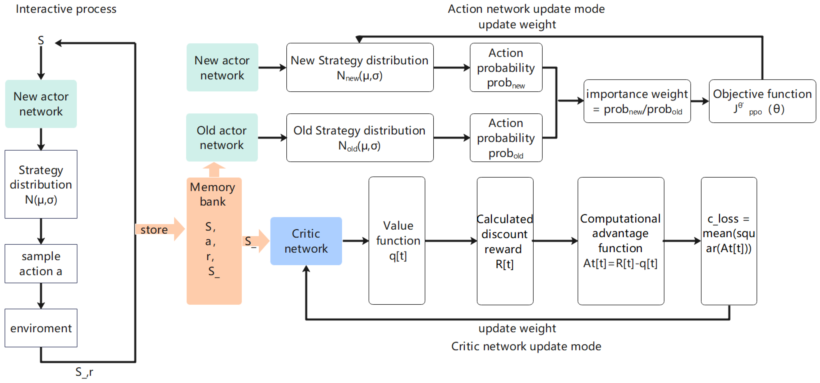
3.2.3. Algorithm Training Process

Figure 1 is the training flow chart of the PPO algorithm:

• Environmental information S is fed into the actor-new network and two values are obtained, one mu and one sigma. These two values are then taken as mean and variance, respectively, to construct a normal distribution, and an action is sampled through this normal distribution.The action is entered into the environment to obtain a reward r and the next state S_, and (S,a,r,S_) is stored as a scheduling experience. Then S_ is entered into the actor-new network, and the previous step is cycled until a certain amount of scheduling experience is stored [26].
• The S_ obtained in the previous step is fed into the critic network, the q_ value of the state is obtained, and the discount reward is calculated. We will get R = [R[0], R[1], …, R[T]].
• All S stored in step 1 are fed into the critic network to obtain all q_ state values, and At = R − q_ is calculated.c_loss = mean (square (At)) is calculated and the critical network parameters are updated by backpropagation.
• All combinations of stored S are entered into the actor-old network and actor-new network to obtain Normal1 and Normal2, respectively. Enter all combinations of stored actions into the normal distributions Normal1 and Normal2 to obtain prob1 and prob2 for each action. Then, the weights of importance are obtained by dividing prob2 by prob1.
• According to Formulas (19) and (20) of the paper, the loss function of the action network is calculated, and then backpropagation is carried out to update the actor-new network.
• Repeat 4–5 steps. After a certain step, the cycle ends. Update the actor-old network with actor-new network weights.
• Repeat 1–6 steps for training until convergence.

Figure 1. PPO algorithm flow chart.

Figure 1. PPO algorithm flow chart.

4. Example Simulation Analysis

The simulation environment is a virtual grid built according to grid data, grid structure and operating rules. The grid has 126 nodes, 35 thermal power units, 18 renewable energy units, 1 balancing unit, 91 loads and 185 load lines. The scheduling interval is 5 min. After the grid is initialized, the grid status quantity is obtained and input to the dispatching policy network to obtain the adjusted value of the active power output of 54 units. The dispatching policy is then fed into the grid environment. The grid is updated to the next state according to the current state quantity and dispatch policy until the end of a dispatch period (one day).

4.1. Model Training Parameter Setting

The network structure uses the full connection layer to build the actor network and the critic network. The state space is 348 dimensions, and the action space is 54 dimensions. The number of hidden layer neurons in the two networks was 512 512 256. The hidden layer uses the ReLU activation function. The learning rate for actor and critic networking was 0.0001 and 0.00001, respectively. The soft update factor for the target network was 0.001, the mini-batch size was 256, and the discount factor was 0.90. Adam optimizer was used to update network parameters. Based on the tensorflow framework, Python is used for training on AMD R5-5500U computers.

Table 1. Neural network structure and parameters.

Network Parameter Setting	Input Layer	First Hidden Layer	Second Hidden Layer	Third Hidden Layer	Output Layer	Learning Rate
Actor network	348	512	512	256	54	0.0001
Critic network	402	512	512	256	1	0.00001

shows the parameters for both networks.

4.2. Data Pre-Processing

Since the distribution range of characteristics of each dimension in the raw data is very different, if the raw data are modeled directly, large numerical scale characteristics will play a more important role in modeling, while small numerical scale characteristics will play a less important or neglected role. Therefore, to ensure the validity and reliability of the model, it is necessary to scale the characteristics of the original data so that the characteristics of each dimension have the same weight as the objective function.

The parameters of the state space and the action space are processed with data standardization respectively.

The same standardized method is used for the active power output of thermal power units ($P_{th,t}$), active power output of renewable energy units ($P_{con,t}$) and active power output of balance units ($P_{bal,t}$). First, the maximum active power output value of three types of units is normalized, and then the value of 54 units is normalized by the L2 norm:

$$\begin{array}{c}\hfill P_{th,norm}=\frac{P_{th,t}}{P_{th,max}}\\ \hfill P_{con,norm}=\frac{P_{con,t}}{P_{con,max}}\\ \hfill P_{bal,norm}=\frac{P_{bal,t}}{P_{bal,max}}\\ \hfill P\in (P_{th,norm},P_{con,norm},P_{bal,com})\\ \hfill P_{norm}=({\frac{P_1}{\Vert P\Vert }}_2,{\frac{P_2}{\Vert P\Vert }}_2,\dots ,{\frac{P_n}{\Vert P\Vert }}_n)\end{array}$$

(21)

The L2 normalization of the branch current load rate ($rh{o}_t$) and the next load demand ($P_{d,t+1}$) is performed:

$$rh{o}_{norm}=({\frac{rh{o}_1}{\Vert rho\Vert }}_2,{\frac{rh{o}_2}{\Vert rho\Vert }}_2,\dots ,{\frac{rh{o}_n}{\Vert rho\Vert }}_n)$$

(22)

$$P_{d,t+1,norm}=({\frac{P_{d,t+1,1}}{\Vert P_{d,t+1}\Vert }}_2,{\frac{P_{d,t+1,2}}{\Vert P_{d,t+1}\Vert }}_2,\dots ,{\frac{P_{d,t+1,n}}{\Vert P_{d,t+1}\Vert }}_n)$$

(23)

For the current maximum output of the renewable energy unit ($P_{th,max,t}$), the maximum allowable output value of the unit is first used for normalization, followed by L2 normalization:

$$\begin{array}{cc}\hfill & P_{th,max,norm}=\frac{P_{th,max,t}}{P_{th,max}}\hfill \\ \hfill & P_{norm}=({\frac{P_{th,max,norm,1}}{\Vert P_{th,max,norm}\Vert }}_2,{\frac{P_{th,max,norm,2}}{\Vert P_{th,max,norm}\Vert }}_2,\dots ,{\frac{P_{th,max,norm,n}}{\Vert P_{th,max,norm}\Vert }}_n)\hfill \end{array}$$

(24)

The output adjustment values of thermal power units, renewable units and balancing units are normalized according to the maximum and minimum output values of each unit, and compressed into [−1,1]:

$$A_{norm}=2\ast \frac{A_t-A_{adjust,min}}{A_{adjust,max}-A_{adjust,min}}-1$$

(25)

4.3. Economic Security Scheduling Decision Model

In this paper, by defining the state space, action space and reward function in the decision-making process, the grid economic security dispatching is modeled as a Markov decision process, which is convenient to use reinforcement learning to solve.

In this paper, a day is defined as a scheduling period, and every 5 min is a scheduling policy. The dispatching system is the agent and the power system is the environment. The agent arranges the unit’s planned output adjustment value by observing the power system environment, and applies the scheduling strategy to the power system environment. The power system environment changes to a new state and returns the reward and punishment situation to the agent to help the agent optimize the scheduling strategy. Loop through the above process until the end of a scheduling cycle.

Each dispatch policy acts on the power system, and the system should return real-time reward function according to the current state to guide the update of the dispatch policy. The objective function and constraints of the renewable power system dispatching model should be reflected in the real-time reward function. Therefore, this paper sets the objective function and constraint conditions in the reward function, which can be divided into reward value and punishment value. When the penalty value is obtained, a negative score is obtained so that such actions violating the constraints can be avoided in subsequent decisions. When the reward value is obtained, the positive score is obtained so that the agent constantly seeks to maximize the real-time reward value to achieve the objective function.

Based on the actual scheduling process, rewards and punishments for scheduling policies are defined:

• The reward of renewable energy consumption:

  $$r1=\sum _{i=1}^{N_{re}}{P}_{i,t}/\sum _{i=1}^{N_{re}}\overline{P_{i,t}}$$

  (26)
• The reward of line overlimit:

  $$r2=1-\frac{1}{N_{line}}\sum _{i=1}^{N_{line}}min(\frac{I_{i,t}}{I_{i,max}+\in },1)$$

  (27)
• The punishment of unit operating cost:

  $$r3=e^{-{\sum }_{i=1}^N(a_i{P}_{i,t}^2+b_i{P}_{i,t}+c_i)-C_{on,off}}-1$$

  (28)
• The punishment of power unbalance:

  $$r4=\left\{\begin{array}{cc}\frac{10}{N_{bal}}\sum _{i=1}^{N_{bal}}1-\frac{p_{bal}}{p_{bal,max}}\hfill & p_{bal,max}<p_{bal}<1.1\ast p_{bal,max}\hfill \\ \frac{10}{N_{bal}}\sum _{i=1}^{N_{bal}}\frac{p_{bal}}{p_{bal,min}}-1\hfill & 0.9\ast p_{bal,min}<p_{bal}<p_{bal,min}\hfill \end{array}\right.$$

  (29)
• The punishment of unit output exceeding the limit:
  Unlike other constraints, there is no need to set a penalty for this constraint, and the unit output adjustment value was limited within the upper and lower limits at the time of setting.
• The punishment of output climbing over the limit of thermal power unit:

  $$r5=\left\{\begin{array}{cc}0\hfill & D_{th,i}\le P_{th,i,t+1}\le U_{th,i}\hfill \\ \frac{U_{th,i}-P_{th,i}}{U_{th,i}}\hfill & P_{th,i,t+1}>U_{th,i}\hfill \\ \frac{D_{th,i}-P_{th,i}}{D_{th,i}}\hfill & P_{tj,i,t+1}<D_{th,i}\hfill \end{array}\right.$$

  (30)
• Real-time reward function:
  Real-time reward function in reinforcement learning plays an important guiding role in agent exploration. Therefore, it is necessary to consider punishment and cost as a whole, define a reasonable reward function, and guide the agent’s strategy in the right direction to update. Combining the above rewards and punishments, set a real-time reward r for scheduling policies:

  $$r=a1\ast r1+a2\ast r2+a3\ast r3+a4\ast r4+a5\ast r5$$

  (31)

  where $r_i$ represents each reward item after normalization, the field values of the reward items r1 and r2 are [0,1], and the field values of the reward items r3, r4 and r5 are [−1,0]. $a_i$ represents the coefficient of each reward item, according to the research emphasis of this paper, a2 = a4 = a5 = 1, a1 = a3 = 2.

4.4. Analysis of Training Results of the Model

The reward value of the single-step scheduling policy is normalized, and the range is [−1,1]. Figure 2 shows the reward value curve of the single-step scheduling strategy along with the training process. As can be seen from the figure, at the beginning, the reward value of the single-step scheduling strategy is between [−0.75,0]. At this time, continuous exploration is carried out in the training process to generate a large amount of scheduling experience to train the model. With the continuous accumulation and training of scheduling experience, the reward value of the single-step scheduling strategy is constantly rising. In the training process, even if the single-step scheduling strategy has reached the optimal level, further exploration is still needed to ensure model convergence. After data normalization, the model was trained 40,000 times with 800,000 scheduling strategies, which took 15 h, and achieved good convergence effect. However, if the data are not normalized to the same scale, it is difficult for model training to converge.

4.5. Analysis of Scheduling Results of the Model

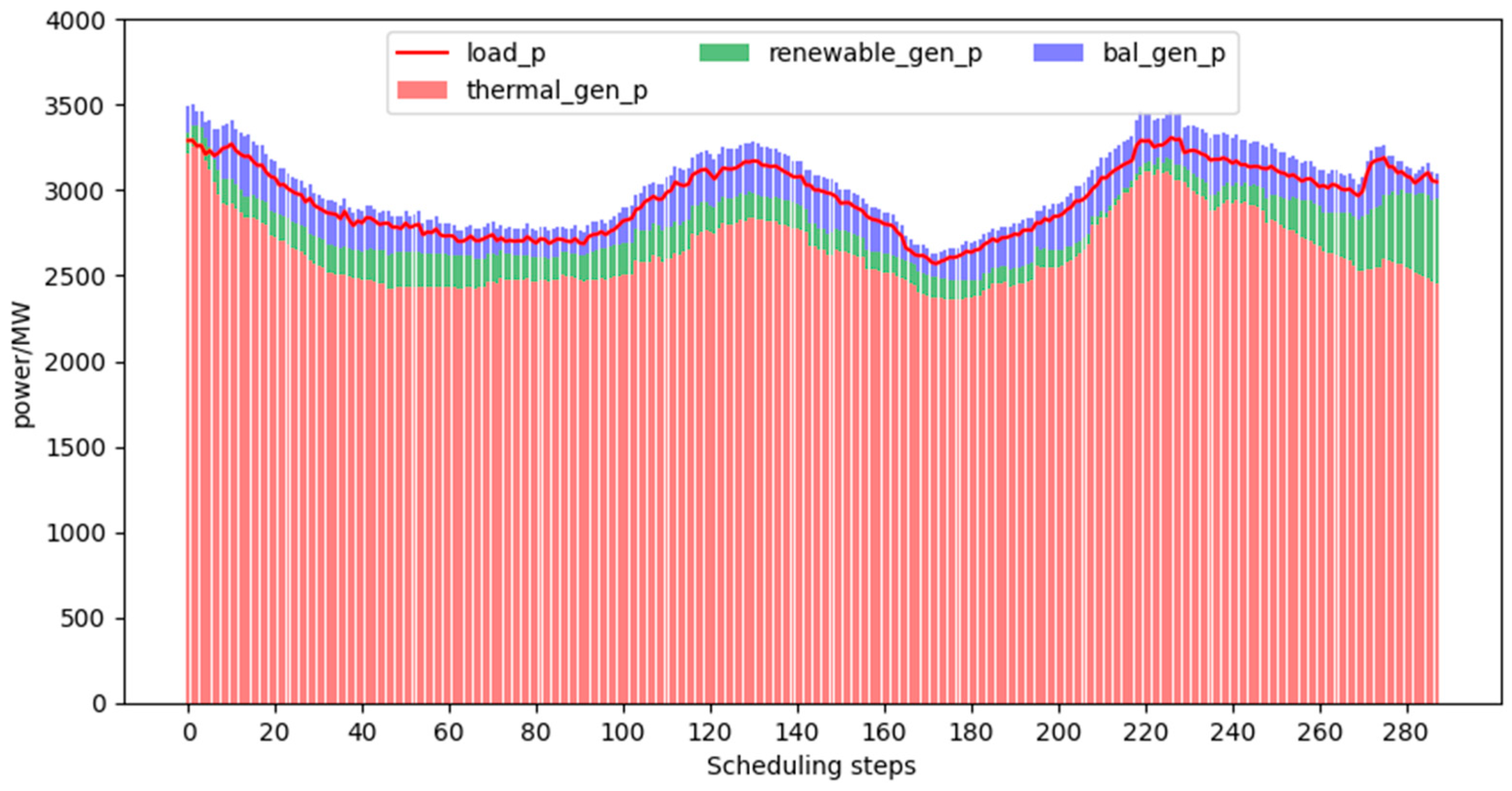
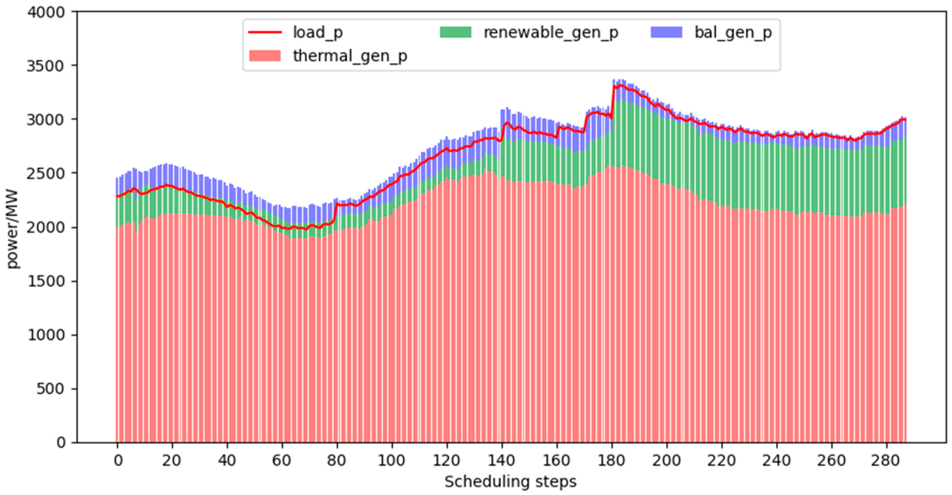
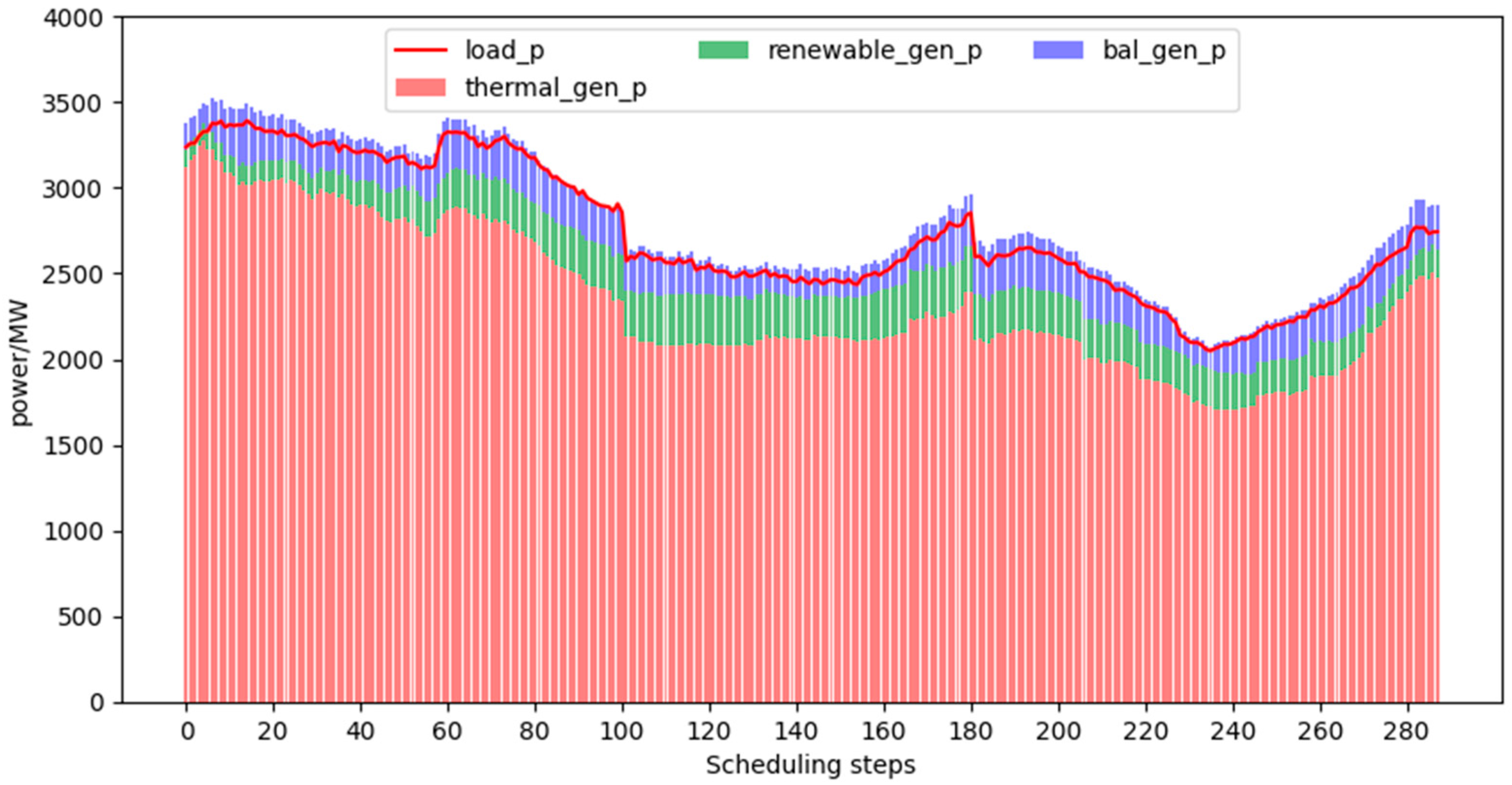
• Analysis of daily scheduling results:
  In the simulation analysis of this paper, a day is set as a scheduling cycle, with a scheduling policy every 5 min. A scheduling cycle provides 288 scheduling policies. The output of each unit in a scheduling cycle with different trends in total loads is shown in Figure 3, Figure 4 and Figure 5.
  Figure 3, Figure 4 and Figure 5 are obtained by the interaction between the scheduling strategy trained by the proximal policy optimization algorithm and the grid environment. As can be seen from the figure, under three different total load scenarios, the output of the balance unit meets the constraints and does not exceed the limit, thus ensuring the smooth operation of the power grid. The unit’s active power output and total load meet the power balance constraints. The variable output range of renewable units is large and the uncertainty is high, which increases the difficulty of scheduling the power system.

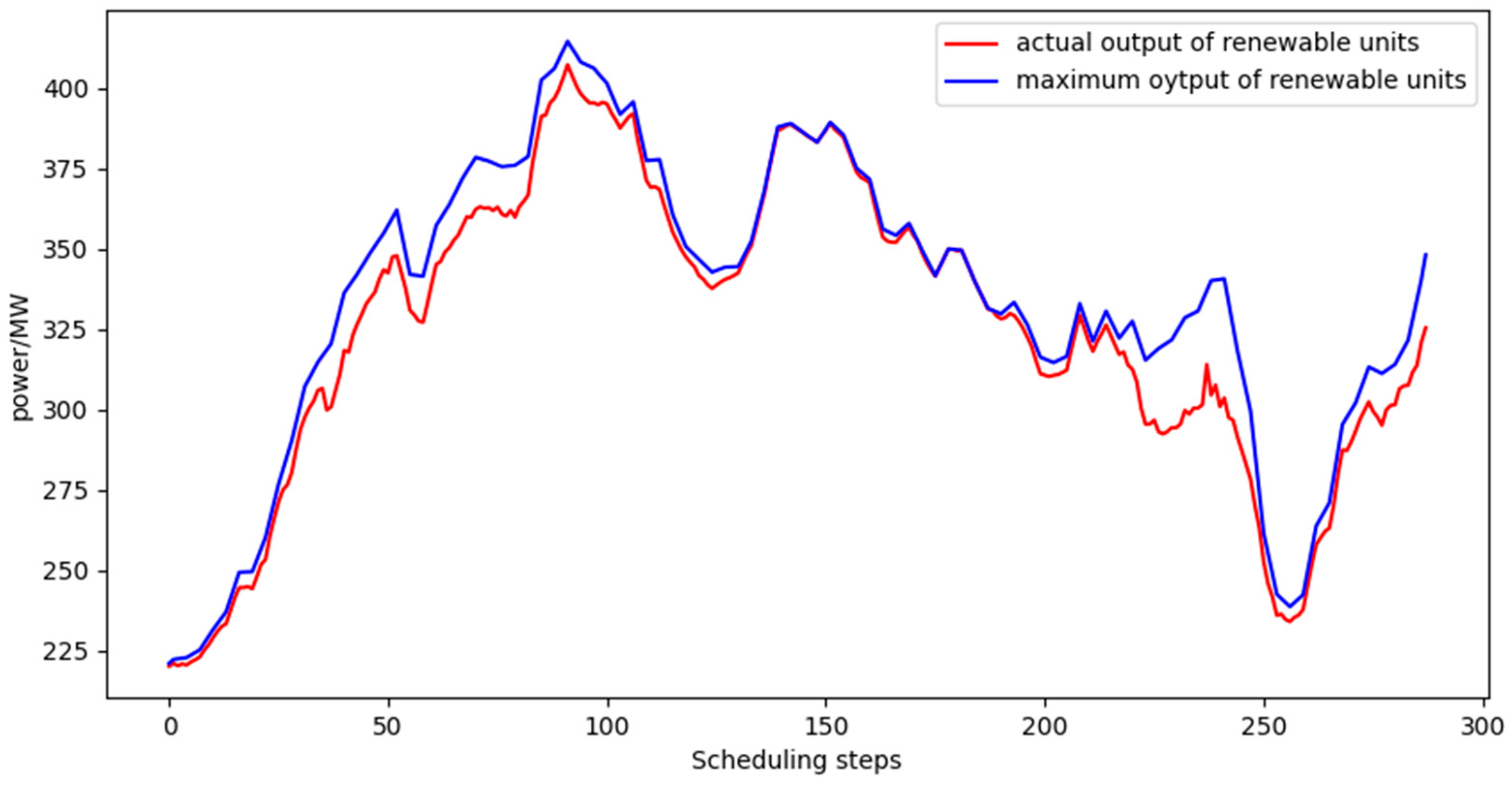
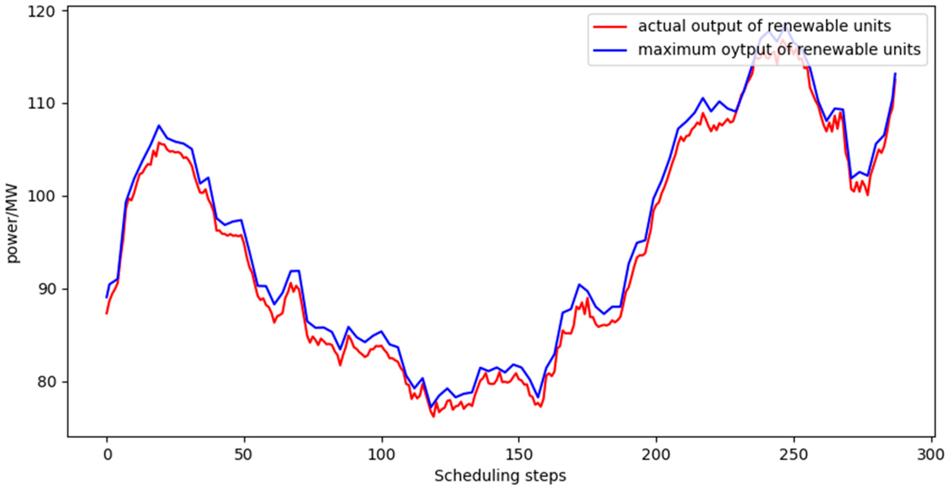
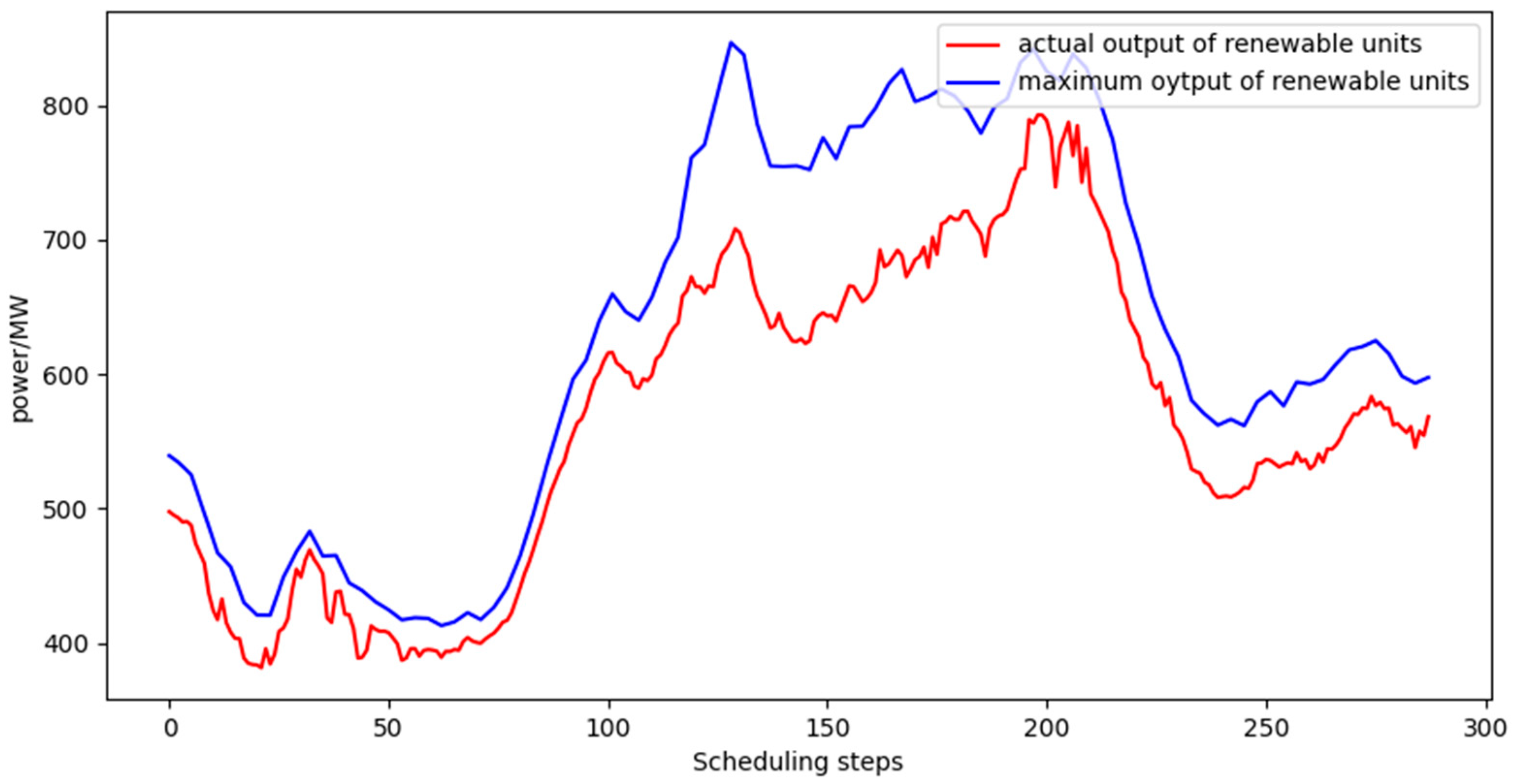
• Analysis of renewable energy consumption.
  The renewable energy consumption rate refers to the ratio of the actual electricity consumed by the generating unit in a dispatch cycle to the electricity generated in the current dispatch cycle. The renewable energy generation rate refers to the ratio of the current renewable energy generation electricity to the maximum generation electricity of the unit. Figure 6, Figure 7 and Figure 8 show the consumption of renewable energy in the three dispatch cycles with different renewable energy generation rates available.

  Table 2. Renewable energy consumption.

  Proportion of Renewable Energy Output	19.8%	50.09%	94.52%
  Renewable energy consumption	98.5%	96.3%	90.1%

  shows the specific renewable energy generation rate and corresponding consumption rates. It can be seen that when the proportion of renewable energy generation is 19.8%, the consumption rate is high and can be effectively absorbed. When the proportion of renewable energy generation is 94.52%, the consumption rate is relatively low. Renewable energy must therefore be used carefully to reduce the impact of uncertainty on grid operation. The dispatch strategy can effectively absorb renewable energy on the premise of ensuring the safe operation of the power grid.

5. Discussion

The method proposed in this paper can effectively deal with the problems caused by a high proportion of renewable energy connected to the grid. However, without the guidance of prior knowledge at the early stage of training, reinforcement learning will face too much exploration space, resulting in overly slow and difficult convergence. Imitation learning can learn from the perfect scheduling strategy to acquire expert knowledge and provide prior knowledge for reinforcement learning so that the perfect scheduling strategy can be imitated in model training, and then its own strategy can be continuously optimized. The discriminator can be used to avoid the artificial setting of the reward function, and the generator can be used to interact with the power system so that the agent can learn a strategy superior to expert experience. This will further improve the convergence of reinforcement learning. Therefore, the economic scheduling strategy of grid security based on generative adversarial imitation learning will be the focus of further research.

6. Conclusions

In this paper, a safe and economical dispatching method for power grids based on the PPO algorithm is proposed. This method considers the safety, economy, renewable energy consumption rate and uncertainty of long-term dispatching. It can effectively address the impact of fluctuating and intermittent renewable energy on the dispatch power system when a high proportion of renewable energy units are connected to the grid. By defining the state space, the action space, and the reward function, the grid scheduling optimization problem is transformed into a Markov decision process. A proximal policy optimization algorithm with the KL divergent penalty factor and important sampling technique is used to solve the Markov decision problem. Finally, a model of 126 node power system is used for simulation. Simulation results show that the proposed method can meet the load requirements of three scheduling cycles under different load trends. The absorption rates of renewable energy were 90.1%, 96.3% and 98.5%, respectively, in the three dispatching periods with different renewable energy generation rates. The effectiveness and applicability of the scheme are proven to ensure the economy of operation of the power system and the absorption of renewable energy.

References

1. Bussar, C.; Stöcker, P.; Cai, Z.; Moraes, L., Jr.; Magnor, D.; Wiernes, P.; van Bracht, N.; Moser, A.; Sauer, D.U. Large-scale integration of renewable energies and impact on storage demand in a European renewable power system of 2050—Sensitivity study. J. Energy Storage 2016, 6, 1–10. [Google Scholar] [CrossRef] [Green Version]
2. Wang, C.; Liu, S.; Bie, Z.; Wang, J. Renewable energy accommodation capability evaluation of power system with wind power and photovoltaic integration. IFAC-PapersOnLine 2018, 51, 55–60. [Google Scholar] [CrossRef]
3. Albadi, M.H.; El-Saadany, E. Overview of wind power intermittency impacts on power systems. Electr. Power Syst. Res. 2010, 80, 627–632. [Google Scholar] [CrossRef]
4. Roald, L.A.; Pozo, D.; Papavasiliou, A.; Molzahn, D.K.; Kazempour, J.; Conejo, A. Power systems optimization under uncertainty: A review of methods and applications. Electr. Power Syst. Res. 2023, 214, 108725. [Google Scholar] [CrossRef]
5. Aien, M.; Hajebrahimi, A.; Fotuhi-Firuzabad, M. A comprehensive review on uncertainty modeling techniques in power system studies. Renew. Sustain. Energy Rev. 2016, 57, 1077–1089. [Google Scholar] [CrossRef]
6. Alqurashi, A.; Etemadi, A.H.; Khodaei, A. Treatment of uncertainty for next generation power systems: State-of-the-art in stochastic optimization. Electr. Power Syst. Res. 2016, 141, 233–245. [Google Scholar] [CrossRef]
7. Tang, C.; Xu, J.; Sun, Y.; Liu, J.; Li, X.; Ke, D.; Yang, J.; Peng, X. Look-ahead economic dispatch with adjustable confidence interval based on a truncated versatile distribution model for wind power. IEEE Trans. Power Syst. 2017, 33, 1755–1767. [Google Scholar] [CrossRef]
8. Ma, M.; He, B.; Shen, R.; Wang, Y.; Wang, N. An adaptive interval power forecasting method for photovoltaic plant and its optimization. Sustain. Energy Technol. Assessments 2022, 52, 102360. [Google Scholar] [CrossRef]
9. Nazari-Heris, M.; Mohammadi-Ivatloo, B. Application of robust optimization method to power system problems. In Classical and Recent Aspects of Power System Optimization; Elsevier: Amsterdam, The Netherlands, 2018; pp. 19–32. [Google Scholar]
10. Xie, W.; Yi, Y.; Zhou, Z.; Wang, K. Data-driven stochastic optimization for power grids scheduling under high wind penetration. Energy Syst. 2020, 14, 41–65. [Google Scholar] [CrossRef]
11. Mieth, R.; Dvorkin, Y. Data-driven distributionally robust optimal power flow for distribution systems. IEEE Control. Syst. Lett. 2018, 2, 363–368. [Google Scholar] [CrossRef] [Green Version]
12. Cherukuri, A.; Cortés, J. Cooperative data-driven distributionally robust optimization. IEEE Trans. Autom. Control. 2019, 65, 4400–4407. [Google Scholar] [CrossRef] [Green Version]
13. Zhang, Z.; Zhang, D.; Qiu, R.C. Deep reinforcement learning for power system applications: An overview. CSEE J. Power Energy Syst. 2019, 6, 213–225. [Google Scholar]
14. Perera, A.; Kamalaruban, P. Applications of reinforcement learning in energy systems. Renew. Sustain. Energy Rev. 2021, 137, 110618. [Google Scholar] [CrossRef]
15. Navin, N.K.; Sharma, R.; Malik, H. Solving nonconvex economic thermal power dispatch problem with multiple fuel system and valve point loading effect using fuzzy reinforcement learning. J. Intell. Fuzzy Syst. 2018, 35, 4921–4931. [Google Scholar] [CrossRef]
16. Li, F.; Qin, J.; Kang, Y. Multi-agent system based distributed pattern search algorithm for non-convex economic load dispatch in smart grid. IEEE Trans. Power Syst. 2018, 34, 2093–2102. [Google Scholar] [CrossRef]
17. Lu, Y.; Xiang, Y.; Huang, Y.; Yu, B.; Weng, L.; Liu, J. Deep reinforcement learning based optimal scheduling of active distribution system considering distributed generation, energy storage and flexible load. Energy 2023, 271, 127087. [Google Scholar] [CrossRef]
18. Dong, J.; Wang, H.; Yang, J.; Lu, X.; Gao, L.; Zhou, X. Optimal scheduling framework of electricity-gas-heat integrated energy system based on asynchronous advantage actor-critic algorithm. IEEE Access 2021, 9, 139685–139696. [Google Scholar] [CrossRef]
19. White, C.C., III; White, D.J. Markov decision processes. Eur. J. Oper. Res. 1989, 39, 1–16. [Google Scholar] [CrossRef]
20. Hausknecht, M.; Stone, P. On-policy vs. off-policy updates for deep reinforcement learning. In Proceedings of the Deep Reinforcement Learning: Frontiers and Challenges, IJCAI 2016 Workshop, New York, NY, USA, 9–15 July 2016; AAAI Press: New York, NY, USA, 2016. [Google Scholar]
21. Cao, D.; Hu, W.; Zhao, J.; Zhang, G.; Zhang, B.; Liu, Z.; Chen, Z.; Blaabjerg, F. Reinforcement learning and its applications in modern power and energy systems: A review. J. Mod. Power Syst. Clean Energy 2020, 8, 1029–1042. [Google Scholar] [CrossRef]
22. Metelli, A.M.; Papini, M.; Faccio, F.; Restelli, M. Policy optimization via importance sampling. arXiv 2018, arXiv:1809.06098. [Google Scholar]
23. Metelli, A.M.; Papini, M.; Montali, N.; Restelli, M. Importance sampling techniques for policy optimization. J. Mach. Learn. Res. 2020, 21, 5552–5626. [Google Scholar]
24. Engstrom, L.; Ilyas, A.; Santurkar, S.; Tsipras, D.; Janoos, F.; Rudolph, L.; Madry, A. Implementation matters in deep policy gradients: A case study on ppo and trpo. arXiv 2020, arXiv:2005.12729. [Google Scholar]
25. Liu, B.; Cai, Q.; Yang, Z.; Wang, Z. Neural trust region/proximal policy optimization attains globally optimal policy. arXiv 2019, arXiv:1906.10306. [Google Scholar]
26. Wang, K.; Peng, H.; Zhao, M.; Guan, W. Collaborative exploration of multiple unmanned surface vessels in complex areas based on PPO algorithm. Journal of Physics: Conference Series. In Proceedings of the 2021 International Conference on Artificial Intelligence, Automation and Algorithms (AI2A 2021), Guilin, China, 23–25 July 2021; IOP Publishing: Bristol, UK, 2021; Volume 2003, p. 012017. [Google Scholar]
Figure 2. Reward value curve of single-step scheduling policy training process.
Energies 16 02926 g002
Figure 3. The scheduling period in which the total load is fluctuant.
Energies 16 02926 g003
Figure 4. The scheduling period in which the total load is increasing.
Energies 16 02926 g004
Figure 5. The scheduling period in which the total load is reduction.
Energies 16 02926 g005
Figure 6. The scheduling period with a fluctuation proportion of the maximum renewable energy output.
Energies 16 02926 g006
Figure 7. The scheduling period with a small proportion of the maximum renewable energy output.
Energies 16 02926 g007
Figure 8. The scheduling period with a large proportion of the maximum renewable energy output.
Energies 16 02926 g008