Research on the Magnetostrictive Characteristics of Transformers under DC Bias

Abstract

Direct current (DC) bias leads to increased vibration and noise in transformers. One of the main causes is the magnetostrictive effect of the transformer core. To address this phenomenon of magnetostriction, firstly, a transmission line model (TLM) of a single-phase transformer under DC bias is developed using transmission line theory and Jiles–Atherton (J–A) ferromagnetic hysteresis theory, taking into account the winding copper loss, core eddy current loss, and leakage effect. Secondly, the time-domain simulation of the single-phase transformer based on the Newton–Raphson iterative method is carried out, and the magnetostriction characteristics of the transformer under different DC and its variation law are analyzed. Finally, the results show that the DC bias results in magnetostrictive distortion and vibration acceleration curve distortion, the left and right wings of the magnetostrictive butterfly curve are no longer symmetrical, the slope of the vibration acceleration image increases significantly, and the degree of distortion is positively correlated with the magnitude of the DC. In addition, the peak values of the magnetostrictive deformation and vibration acceleration become larger under DC bias, leading to an increase in the vibration and noise of the transformer. The research object of this paper is the single-phase transformer, and the research method can also be applied to the study of three-phase transformers.

1. Introduction

Power transformers are hubs for the long-distance transmission and distribution of electrical energy in a power grid system, and their safe operation is crucial for the reliability of the entire system. The following reasons can cause DC bias in transformers. The first reason is that due to solar magnetic storms causing changes in the geomagnetic field, potential differences are induced on the Earth’s surface, resulting in geomagnetic-induced currents (with a frequency less than 0.01 Hz, which can be approximated as direct current). The second cause is the application of high-voltage direct current transmission technology, which often operates in a unipolar earth circuit or bipolar unbalanced mode. The direct current in the Earth’s return current will flow into a transformer, winding through the grounding neutral point of the AC transformer, generating a direct current component in the excitation current. The third reason is urban rail transit, which mostly uses direct current to drive vehicles. Its direct current power supply takes the Earth as one of its poles, similar to the unipolar operation of direct current transmission, causing direct current bias in the large transformers of a city. DC bias will aggravate transformer vibration and noise [1,2,3]. The magnetostriction of a transformer’s core is one of the main reasons [4,5]. Under DC bias, the iron core of a transformer quickly enters a saturated state, causing the working point to shift, seriously affecting its normal operation. The phenomenon of DC bias in transformers has attracted much attention. Therefore, it is necessary to study the effect of DC bias on the magnetostriction of transformer cores.

Magnetostriction is the change in the size of ferromagnetic materials caused by magnetization. It is a significant feature of ferromagnetic materials. DC bias magnetism has an effect on the magnetostrictive properties of a transformer’s core. The most intuitive hazard is that it increases the deformation of a transformer’s core, which leads to an increase in its vibration noise. So far, scholars have conducted a large amount of research on this topic.

Professor Philip I. Anderson of the UK and Professor Enokizono of Japan used triaxial strain gauges to measure the magnetostrictive characteristics of silicon steel sheets (SSS) during alternating and rotating magnetization [6]. In References [7,8], to improve the accuracy of the measurements of the micro-deformation of magnetostriction, the vector magnetostrictive characteristics of SSS in the alternating magnetization mode and in the AC/DC hybrid mode were studied using the laser measurement method. In Reference [9], using the measured magnetostrictive curves of SSS, the magnetostrictive force of the EHV transformer core at different times was calculated; then, the intensity and distribution of the vibration and noise were analyzed using the magnetostrictive force and thermal stress. He Qiang et al. measured and analyzed the modal vibration and noise of a 110 kV transformer core without load and pointed out that the magnitude of the vibration and noise differed because of the magnetostrictive anisotropy in various parts of the core. The vibration and noise of transformer’s core are strongly affected by the modal characteristics [10]. By considering the influence of stress on the movement of a saturated domain wall and the hysteresis characteristics, Ben Tong et al. noted that the magnetostrictive model of non-oriented electrical SSS improved in view of the force-magnetic coupling effect, and the influence of pre-stress on the magnetostrictive strain was also studied [11].

Zhang Li et al. established an essential magnetostrictive model of grain-oriented SSS from the viewpoint of the micromagnetic domain and macro thermodynamics. Then, combined with the elasticity theory, the vibration model of a transformer core was built and the deformation caused by magnetostriction was simulated and analyzed [12]. Hu Jingzhu et al. established their electromagnetic–structural–acoustic field finite element model. Through a transient electromagnetic field analysis, the time-domain waveform of the electromagnetic force on the core and winding was obtained. The vibration displacement of each node on the surface of the core and winding was obtained through a vibration analysis in the frequency domain, and it was used as the boundary condition for the transformer sound field analysis [13]. Li Bing et al. conducted a no-load and load DC bias tests using two 250 MVA/500 kV transformers with the same parameters, and they measured the voltage distortion rate, excitation current, vibration, and noise under the DC bias of the transformers. The voltage distortion rate, excitation current, vibration, and noise under the DC bias of the transformer were measured, and the trend, distribution law, and spectral characteristics under the DC bias were analyzed and studied [14]. Research on the magnetostrictive characteristics of transformer cores is mostly focused on experimental measurements. There are few studies on the magnetostriction of transformer cores conducted through modeling and simulation and even fewer via DC bias. In addition, few studies are conducted through simulation and calculation using variation rules of magnetostrictive features of transformer cores when the DC intrudes into the winding from a neutral point.

J–A theory is widely used in the modeling of magnetic materials, which has the advantages of conforming to the physical essence of magnetic hysteresis, fewer parameters, and easy implementation. The circuit equation in the mathematical model of the transformer contains a large number of differential terms, and the process of the solution is complex. Transmission line theory can discrete these differential terms. In this paper, we combined J–A theory with transmission line theory. The TLM of a single-phase transformer under DC bias was built using transmission line theory and J–A theory. The electromagnetic characteristics of a transformer in the time domain was simulated, and the magnetostrictive curves under different DC bias were obtained using the Newton–Raphson iterative method. The variation rules with DC were analyzed. In addition to calculating the saturation and hysteresis effects of the iron core, the model also considered factors such as eddy current loss, winding copper loss, and magnetic leakage of the iron core to fully and completely describe the single-phase transformer under DC bias [15].

2. J–A Theory

There are two key points in transformer modeling. The first is the representation of the magnetization curve, and the second is the conversion of the magnetic circuit to a circuit.

The operating characteristics of a DC bias transformer are closely related to the electromagnetic properties of the material. Therefore, the study of the magnetic properties of core materials under AC–DC coexistence excitation is the key and prerequisite to solving the DC bias magnetization problem [16]. Jiles–Atherton theory describes the nonlinearity of ferromagnetic materials from the physical mechanism of ferromagnetic materials; that is, it describes the relationship between magnetization, $M$, and magnetic field’s strength, $H$. Jiles–Atherton theory decomposes magnetization into two components: irreversible, $M_{\mathrm{irr}}$, and reversible, $M_{\mathrm{rev}}$.

$$M=M_{\mathrm{irr}}+M_{\mathrm{rev}}$$

(1)

The J–A model combines the microstructural parameters of magnetic materials with macroscopic characterization, which is more consistent with the physical nature of the hysteresis phenomenon. $M_{\mathrm{irr}}$ is caused by the friction effect between magnetic domains, and $M_{\mathrm{rev}}$ is caused by the elastic bending of the domain wall. According to Jiles–Atherton theory, the internal magnetization curve can be defined as:

$$M_{\mathit{an}}=M_{s}f(H_e)$$

(2)

Among them, $H_e=H+\alpha M$, and $\alpha$ is the coupling coefficient in the domain, and $M_s$ is the saturation magnetization.

Using the modified Langvin function, $f(H_e)$ can be obtained.

$$\begin{array}{l}f(H_e)=\frac{a_1{H}_e+{H_e}^b}{a_3+a_2{H}_e+{H_e}^b}\\ a_2>a_1,b>1,a_1,a_2,a_3>0\end{array}$$

(3)

In order to reach the last set of solvable equations to construct the $M/H_e$ and $B/H$ curves, it is necessary to establish the basic Relationship (4).

$$\frac{dM}{dH}=\frac{c\frac{d{M}_{an}}{d{H}_e}+\frac{M_{an}-M}{\frac{\delta k}{{\mu }_0}-\frac{\alpha (M_{an}-M)}{1-c}}}{1-ac\frac{d{M}_{an}}{d{H}_e}}$$

(4)

where $\alpha$, $c$, and $k$ are constants dependent on the material used, ${\mu }_0$ is the vacuum permeability, and $\delta$ is related to $\frac{dH}{dt}$ that take 1 or −1.

If $(M_{an}-M)·\delta <0$, adopt a modified form of (5).

The derivative of $M_{an}$ with respect to $H_e$ gives Equation (6).

$$\frac{dM}{dH}=\frac{c\frac{d{M}_{an}}{d{H}_e}}{1-ac\frac{d{M}_{an}}{d{H}_e}}$$

(5)

$$\frac{d{M}_{an}}{d{H}_e}=M_s\frac{a_1+\frac{b{H_e}^b}{H_e}}{a_3+a_2{H}_e+{H_e}^b}-M_s\frac{(a_1{H}_e+{H_e}^b)(a_2+\frac{b{H_e}^b}{H_e})}{{(a_3+a_2{H}_e+{H_e}^b)}^2}$$

(6)

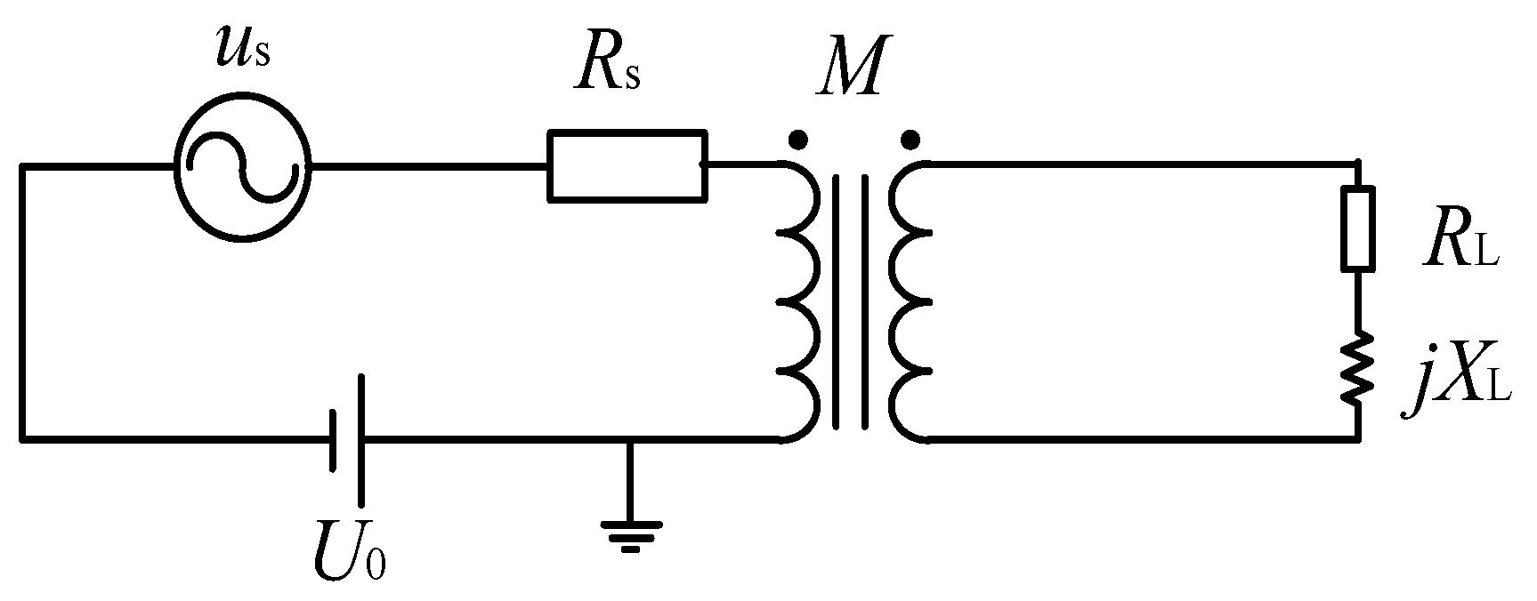
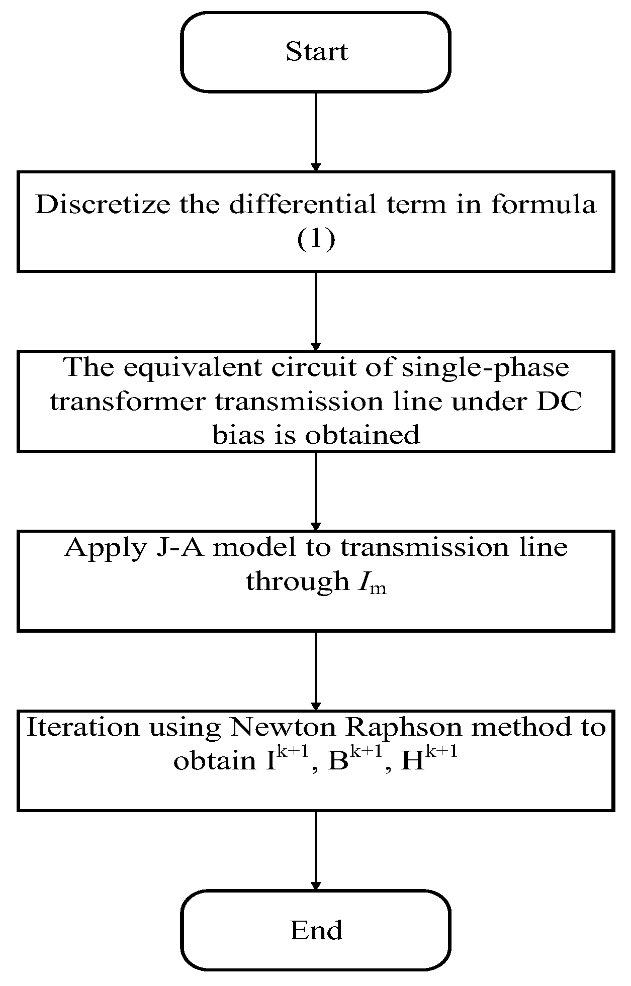
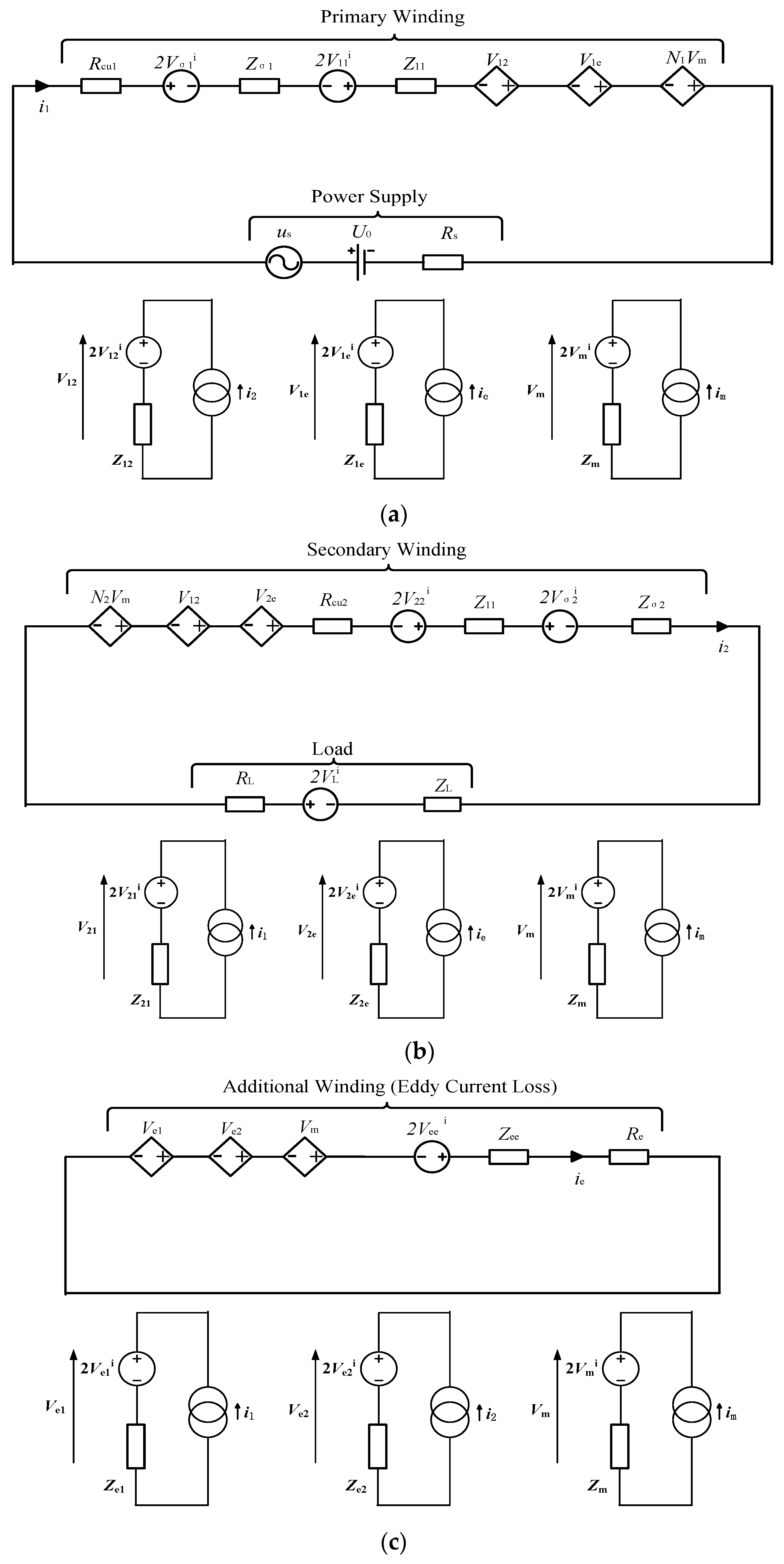
3. TLM of a Single-Phase Transformer

The circuit model is shown in Figure 1 and Equation (7). In this model, u_s represents the AC power supply voltage; U₀ represents the rising ground potential of the transformer grounding point; R_s represents the internal resistance of the power supply; M represents the nonlinear mutual inductance; and Z_L represents the secondary side load; the magnetic hysteresis effect and the magnetic leakage effect, copper loss, and eddy current loss are also considered. The eddy current loss can be replaced by adding a single-turn coil with resistance (i.e., the additional winding and resistance) which is mutually inductive to the primary and secondary winding. The calculation process is shown in Figure 2.

$$\left\{\begin{array}{c}{u}_s+U_0=R_s{i}_1+R_{\mathrm{cu}1}{i}_1+L_{\mathsf{\sigma }1}\frac{\mathrm{d}{i}_1}{\mathrm{d}t}+L_{11}\frac{\mathrm{d}{i}_1}{\mathrm{d}t}+M_{12}\frac{\mathrm{d}{i}_2}{\mathrm{d}t}+M_{1\mathrm{e}}\frac{\mathrm{d}{i}_{\mathrm{e}}}{\mathrm{d}t}+N_1{L}_{\mathrm{m}}\frac{\mathrm{d}{i}_{\mathrm{m}}}{\mathrm{d}t}\\ 0=R_{\mathrm{cu}2}{i}_2+L_{\mathsf{\sigma }2}\frac{\mathrm{d}{i}_2}{\mathrm{d}t}+L_{22}\frac{\mathrm{d}{i}_2}{\mathrm{d}t}+M_{21}\frac{\mathrm{d}{i}_1}{\mathrm{d}t}+M_{2\mathrm{e}}\frac{\mathrm{d}{i}_{\mathrm{e}}}{\mathrm{d}t}+N_2{L}_{\mathrm{m}}\frac{\mathrm{d}{i}_{\mathrm{m}}}{\mathrm{d}t}+R_{\mathrm{L}}{i}_2+L_{\mathrm{L}}\frac{\mathrm{d}{i}_2}{\mathrm{d}t}\\ 0=L_{\mathrm{ee}}\frac{\mathrm{d}{i}_{\mathrm{e}}}{\mathrm{d}t}+M_{\mathrm{e}1}\frac{\mathrm{d}{i}_1}{\mathrm{d}t}+M_{\mathrm{e}2}\frac{\mathrm{d}{i}_2}{\mathrm{d}t}+L_{\mathrm{m}}\frac{\mathrm{d}{i}_{\mathrm{m}}}{\mathrm{d}t}+R_{\mathrm{e}}{i}_{\mathrm{e}}\end{array}\right.$$

(7)

The additional resistance is:

$$R_{\mathrm{e}}=\frac{12A^2}{t^2{\mathsf{\sigma }}_{\mathrm{fe}}{V}_{\mathrm{c}}{K}_{\mathrm{fe}}}$$

(8)

According to the transmission line theory of nonlinear inductance, the differential terms in Equation (7) are discretized to obtain the equivalent circuits for the TLM under DC bias, as shown in Figure 3.

Considering the hysteresis characteristics of the transformer core, the typical J–A model [17,18,19,20,21] is represented in the following equations:

$$\begin{gathered} i_{\mathrm{m}}={\beta }_c{i}_{\mathit{an}}+(1-{\beta }_c)i_{\mathrm{irr}} \\ {i}_{\mathit{an}}=i_s\left[\mathit{cot}h(\frac{i_h+\alpha i_{\mathrm{m}}}{a})-\frac{a}{i_h+\alpha i_{\mathrm{m}}}\right] \\ \frac{d{i}_{\mathrm{irr}}}{d{i}_h}=\frac{{\delta }_M(i_{\mathit{an}}-i_{\mathrm{irr}})}{\delta i_c-\alpha (i_{\mathit{an}}-i_{\mathrm{irr}})} \\ \frac{d{i}_{\mathit{an}}}{d{i}_h}=\frac{i_s}{a}\left[-\frac{2}{\mathit{sin}h(\frac{i_h+\alpha i_{\mathrm{m}}}{a}{)}^2}+(\frac{a}{i_h+\alpha i_{\mathrm{m}}}{)}^2\right] \\ \frac{\mathrm{d}{i}_{\mathrm{m}}}{\mathrm{d}{i}_h}={\beta }_c\frac{\mathrm{d}{i}_{\mathit{an}}}{\mathrm{d}{i}_h}+{\delta }_{\mathrm{M}}(1-{\beta }_c)\frac{\mathrm{d}{i}_{\mathrm{irr}}}{\mathrm{d}{i}_h} \end{gathered}$$

(9)

where δ is related to $\frac{d{i}_h}{dt}$. When $\frac{d{i}_h}{dt}>0,\delta =1$. When $\frac{d{i}_h}{dt}<0,\delta =-1$. The migration flag δ_M is given by:

$${\delta }_{\mathrm{M}}=\left\{\begin{array}{cc}1,& \mathrm{if}\delta \mathrm{and}{i}_{\mathit{an}}>i_{\mathrm{irr}}\\ 1,& \mathrm{if}\delta \mathrm{and}{i}_{\mathit{an}}<i_{\mathrm{irr}}\\ 0,& \mathrm{otherwise}\end{array}\right.$$

(10)

4. Results

4.1. Solution of the TLM

The J–A theory of the TLM of the single-phase transformer uses i_m. Then, Newton–Raphson iterative method is used to solve it. The simultaneous equations are presented for an iterative solution in consideration of the nonlinear magnetizing current i_m:

$$\left\{\begin{array}{cc}{f}_1=& (R_{\mathrm{S}}+R_{\mathrm{cu}1}+Z_{11}+Z_{\mathsf{\sigma }1})i_1+Z_{12}{i}_2+Z_{1\mathrm{e}}{i}_{\mathrm{e}}+N_1{Z}_{\mathrm{m}}{i}_{\mathrm{m}}-u_{\mathrm{s}}\\ & -U_0+2({V_{11}}^{\mathrm{i}}+{V_{\mathsf{\sigma }1}}^{\mathrm{i}}+{V_{12}}^{\mathrm{i}}+{V_{1\mathrm{e}}}^{\mathrm{i}}+N_1{V_{\mathrm{m}}}^{\mathrm{i}})\\ f_2=& (R_{\mathrm{L}}+R_{\mathrm{cu}2}+Z_{22}+Z_{\mathsf{\sigma }2}+Z_{\mathrm{L}})i_2+Z_{21}{i}_1+Z_{2\mathrm{e}}{i}_{\mathrm{e}}+N_2{Z}_{\mathrm{m}}{i}_{\mathrm{m}}\\ & +2({V_{22}}^{\mathrm{i}}+{V_{\mathsf{\sigma }2}}^{\mathrm{i}}+{V_{21}}^{\mathrm{i}}+{V_{2\mathrm{e}}}^{\mathrm{i}}+N_2{V_{\mathrm{m}}}^{\mathrm{i}})\\ f_3=& (R_{\mathrm{e}}+Z_{\mathrm{ee}})i_{\mathrm{e}}+Z_{\mathrm{e}1}{i}_1+Z_{2\mathrm{e}}{i}_2+Z_{\mathrm{m}}{i}_{\mathrm{m}}+2({V_{\mathrm{ee}}}^{\mathrm{i}}+{V_{\mathrm{e}1}}^{\mathrm{i}}+{V_{\mathrm{e}2}}^{\mathrm{i}}+{V_{\mathrm{m}}}^{\mathrm{i}})\end{array}\right.$$

(11)

where f₁ = f₂ = f₃ = 0, and the Jacobian matrix is given by:

$$J=\left[\begin{array}{ccc}\frac{\partial f_1}{\partial i_1}& \frac{\partial f_1}{\partial i_2}& \frac{\partial f_1}{\partial i_{\mathrm{e}}}\\ \frac{\partial f_2}{\partial i_1}& \frac{\partial f_2}{\partial i_2}& \frac{\partial f_2}{\partial i_{\mathrm{e}}}\\ \frac{\partial f_3}{\partial i_1}& \frac{\partial f_3}{\partial i_2}& \frac{\partial f_3}{\partial i_{\mathrm{e}}}\end{array}\right]$$

(12)

Then, the current can be calculated:

$${\left[\begin{array}{c}{i}_1\\ i_2\\ i_{\mathrm{e}}\end{array}\right]}_{k+1}={\left[\begin{array}{c}{i}_1\\ i_2\\ i_{\mathrm{e}}\end{array}\right]}_k-{\left[J\right]}_k^{-1}{\left[\begin{array}{c}{f}_1\\ f_2\\ f_3\end{array}\right]}_k$$

(13)

where k is the number of iteration steps.

Next, i_m^k+1 is given by:

$$\begin{array}{cc}{i}_{\mathrm{m}}{}^{k+1}=\hfill & {\left\{\begin{array}{c}{u}_{\mathrm{s}}+U_0-\left(R_{\mathrm{s}}+R_{\mathrm{cu}1}+X_{22}+X_{\mathsf{\sigma }1}\right)i_1+Z_{12}{i}_2+Z_{1\mathrm{e}}{i}_{\mathrm{e}}\hfill \\ \frac{+2\left(V_{11}{}^{\mathrm{i}}+V_{\mathsf{\sigma }1}{}^{\mathrm{i}}+V_{12}{}^{\mathrm{i}}+V_{1\mathrm{e}}{}^{\mathrm{i}}+N_1{V}_{\mathrm{m}}{}^{\mathrm{i}}\right)}{3N_1{Z}_m}\hfill \end{array}\right\}}_{k+1}\\ \hfill -& {\left\{\begin{array}{c}\left(R_{\mathrm{L}}+R_{\mathrm{cu}2}+Z_{22}+Z_{\mathsf{\sigma }2}+Z_{\mathrm{L}}\right)i_2+Z_{21}{i}_1+Z_{2\mathrm{e}}{i}_{\mathrm{e}}\hfill \\ \frac{+2\left(V_{22}{}^{\mathrm{i}}+V_{\mathsf{\sigma }2}{}^{\mathrm{i}}+V_{21}{}^{\mathrm{i}}+V_{2\mathrm{e}}{}^{\mathrm{i}}+N_2{V}_{\mathrm{m}}{}^{\mathrm{i}}\right)}{3N_2{Z}_m}\hfill \end{array}\right\}}_{k+1}\hfill \\ \hfill -& {\left\{\frac{\left(R_{\mathrm{e}}+Z_{\mathrm{ee}}\right)i_{\mathrm{e}}+Z_{\mathrm{e}1}{i}_1+Z_{\mathrm{e}2}{i}_2+2\left(V_{\mathrm{ee}}{}^{\mathrm{i}}+V_{\mathrm{e}1}{}^{\mathrm{i}}+V_{\mathrm{e}2}{}^{\mathrm{i}}+V_{\mathrm{m}}{}^{\mathrm{i}}\right)}{3Z_m}\right\}}_{k+1}\hfill \end{array}$$

(14)

The iteration begins from the starting values of the previous time step and tends to the appropriate convergence. Here, the criteria is set as:

$$\left|{(i_1)}_{k+1}-{(i_1)}_k\right|<\gamma \mathrm{and}\left|{(i_2)}_{k+1}-{(i_2)}_k\right|<\gamma \mathrm{and}\left|{(i_{\mathrm{m}})}_{k+1}-{(i_{\mathrm{m}})}_k\right|<\gamma$$

(15)

where γ is the convergence parameter (γ = 10⁻⁷). H^k+1 and B^k+1 are further calculated:

$$\begin{array}{cc}{H}^{k+1}=& \frac{N_1{i_1}^{k+1}+N_2{i_2}^{k+1}}{l}\\ B^{k+1}=& \frac{\mu }{l}(N_1{i_1}^{k+1}+N_2{i_2}^{k+1}+{i_m}^{k+1})\end{array}$$

(16)

After calculating the H and B, the deformation Δl caused by magnetostriction is finally solved:

$$\Delta l=l{\displaystyle {\int }_0^H\left|H\right|}\frac{2{\lambda }_{\mathrm{s}}}{{H_{\mathrm{c}}}^2}\mathrm{d}H$$

(17)

According to magnetostrictive deformation Δl, the acceleration g of the core vibration can be obtained:

$$g=\frac{v}{t}=\frac{{\mathrm{d}}^2(\Delta l)}{\mathrm{d}{t}^2}$$

(18)

4.2. Calculation Results

According to the TLM method described above, a small 33.3 kVA, 220/5774 V power transformer was modeled. MATLAB software was used to simulate under DC bias. The voltage applied was U_msinωt(1-e^−20t)V(U_m = 220 V).

Table 1. Name plate parameters of the power transformer.

Parameter Magnitude
Rated capacity: 33.3 KVA
Rated voltage: 230/5774 V
Rated current: 3.3/83.3 A
No load loss: 0.204 kw
Coil turns: 60/1575
Short circuit impedance: 4%
Original winding resistance: 0.0087 Ω
Original winding inductance: 0.4 mH
Secondary winding resistance: 13 Ω
Secondary winding inductance: 254.7 mH

shows the parameters of the single-phase transformer studied. The rated current was 3.3/83.3 A, the no-load loss was 0.204 kw, the number of turns was 60/1575, the short-circuit impedance was 4%, the primary winding resistance was 0.0087 Ω, the primary winding inductance was 0.4 mH, the secondary winding resistance was 13 Ω, and the secondary winding inductance was 254.7 mH.

Figure 4 shows the curves of Δl-H and Δl-B for the slow start simulation when the power voltage increased to the nominal value. It can be seen that the curves presented butterfly shapes, which indicates that the changes of the Δl lagged behind the changes of the magnetic field. There was an obvious intersection between the left and right wings at the zero longitudinal axis in Figure 4a. This means that the deformation still existed when H was zero, i.e., Δl was not equal to zero. In Figure 4b, the intersection point is relatively low and close to the horizontal axis. The left and right wings of the curves are symmetrical at the magnetic field, and the range boundaries are consistent with each other when there is no DC bias. The lines inside the boundaries show that the wings gradually became larger, which suggests that the magnetostrictive deformation enlarged as the applied AC voltage increased.

Figure 5 shows the B-H and Δl-H curves when the AC voltage peak U_m increased. It can be observed that the two curves were obviously bent when the magnetic field’s intensity exceeded 800 A/m, which indicates that the increasing tendency of the magnetic flux density and magnetostrictive deformation obviously weakened. Therefore, the magnetostrictive phenomenon also has saturation characteristics, because the elongation and contraction of the internal magnetic domain were significantly reduced as H reached a certain value. This indicates that from a micro perspective, when the magnetic field intensity increases to a certain value, the elongation and contraction of the internal magnetic domains significantly decrease, and the magnetization direction of the magnetic moments in all magnetic domains gradually aligns with the direction of the external magnetic field, reaching a magnetic saturation state.

Figure 6 illustrates the waveform of the vibration acceleration without DC bias. Figure 6a shows that the fundamental frequency of the waveform was 100 Hz, indicating that compared with the applied voltage frequency, the vibration frequency doubled. In addition, the acceleration amplitude became larger with the increase in the AC voltage, and the waveform was symmetrical about the transverse axis. Figure 6b shows that when the frequency was 100 Hz, the amplitude of the vibration acceleration reached the maximum, which means that the vibration signal changed most violently at this frequency.

Figure 7 shows the curves of the relationship between the magnetostrictive deformation and the magnetic field with DC bias. Figure 7a shows the variation of the magnetostrictive deformation with magnetic field’s strength and the flux density when the DC bias current is −0.15 A. The DC bias current here is approximately 4.5% of the rated current. Figure 7b shows the variation of the magnetostrictive deformation with the magnetic field’s strength and flux density when the DC bias current is −0.25 A. The DC bias current here is approximately 7.6% of the rated current. It can be observed that the left and right wings of the curves lose symmetry, indicating that distortion occurred. The range boundaries of the right wings significantly reduced and tended to degrade. This means that the amplitudes of the magnetic field and deformation decreased. The left wings, however, changed in the opposite direction. With the increase in DC, the asymmetry became increasingly obvious. When the DC was −0.25 A, the maximum amplitudes of the magnetic field and deformation of the left wing were approximately 1.04 and 1.1 times that without DC bias, respectively. The differences between the maximum amplitudes of the left and right wings also increased, as shown in

Table 2. Comparison of the maximum amplitude with and without DC bias.

	Maximum Amplitudes without DC	Differences of Maximum Amplitudes of Left and Right Wings without DC	Maximum Amplitudes of Right Wing when DC Is −0.25 A	Maximum Amplitudes of Left Wing when DC Is −0.25 A	Differences of Maximum Amplitudes of Left and Right Wings when DC Is −0.25 A
Hmax (A/m)	632	1264	620	−656	1276
Bmax (T)	1.57	3.14	1.51	−1.64	3.15
∆lmax (m)	2.94199 × 10−6	0	2.92392 × 10−6	3.14789 × 10−6	0.22397 × 10−6

. Moreover, the boundaries of the curves scattered under different AC voltages. This suggests that the sensitivity of the deformation to the change in the AC signal enhanced; that is, the change in the magnetostriction is more obvious with the increase in the AC voltage due to the existence of DC bias. In addition, the intersections of the left and right wings deviated from the zero longitudinal axis, indicating that the DC bias affected the hysteresis of the deformation relative to the magnetic field.

Table 2 provides a summary of the above simulation results. From Table 2, we can see that when there was no DC, the maximum value of the magnetic field’s strength was 632 A/m, the maximum value of the magnetic flux density was 1.57 T, and the maximum value of the magnetostrictive deformation was 2.94199 × 10⁻⁶ m. The difference in the amplitude between the left and right wings was as follows: magnetic field’s strength was 1264 A/m, magnetic flux density was 3.14 T, and magnetostrictive deformation was 0 m. When the DC increased to −0.25 A, the maximum amplitude of the right wing was 620 A/m, the magnetic flux density was 1.51 T, and the magnetostrictive deformation was 2.92392 × 10⁻⁶ m. The maximum amplitude of the left wing was −656 A/m, the magnetic induction was −1.64 T, and the magnetic induction was 3.14789 × 10⁻⁶ m. The data in the table show more clearly that the magnetostriction shifts some electromagnetic characteristics of the transformer, shifts the hysteresis line, and changes the flux density and magnetic field’s strength magnitude. The magnetostriction butterfly curve was no longer symmetrical between the two wings, and the peaks of the left and right wings deviated. This shows that the DC bias magnetism affected the hysteresis and saturation of the transformer core.

When the DC was −0.25 A, the difference between the maximum amplitude of the left and right wings was shown as follows: magnetic field’s strength was 1276 A/m, the magnetic flux density was 3.15 T, and the magnetostrictive deformation was 0.22397 × 10⁻⁶ m.

Figure 8 depicts the waveform of the vibration acceleration when the DC was −0.25 A. It can be found from Figure 8a that the time-domain waveform of the acceleration was no longer symmetrical about the transverse axis, and the amplitudes of the negative half of the axis were greater than that of the positive half of the axis. This is because the added DC was negative. The maximum amplitude of the acceleration increased to 0.5078 m/s², which is approximately 1.12 times that of when there was no DC bias. In Figure 8b the amplitude of the vibration acceleration was still concentrated at 100 Hz. It reached 0.24224 m/s², which is 1.09 times that of when there was no DC bias. In addition, due to the influence of the DC bias, a small wave peak appeared at 50 Hz. This shows that DC bias magnetism causes an increase in the peak value of the transformer core’s vibration acceleration and a new peak value at other frequencies. Therefore, the DC bias magnetism has an effect on the transformer vibration, and DC bias magnetism enhances the vibration of the transformer.

Figure 9a,b illustrate that the curves of the magnetic field changed with the DC. As can be observed from Figure 8a, when the DC was less than 0.1 A, the magnetic field’s strength slowly changed with the increase in the DC. When the DC was greater than 0.1 A and less than 0.3 A, the magnetic field’s strength gradually increased with the increase in the DC. When the DC was 0.1 A, the magnetic field’s strength was 638.87 A/m, when the DC was 0.3 A, the magnetic field’s strength was 681.02 A/m. There was an inflection point of the curve when the DC was 0.3 A. The curve became steeper, and the magnetic field’s strength increased rapidly, as it was greater than 0.3 A, which suggests that the influence of the DC on the magnetic field’s strength was obviously strengthened. Figure 9b shows that the variation curve of the magnetic flux density with the DC results in a straight line, and with the increase in the direct current, the magnetic flux density changed linearly.

Figure 9c,d show the variation curves of the magnetostrictive deformation and the vibration acceleration with the DC, respectively. When the DC was less than 0.1 A, both the magnetostrictive deformation and vibration acceleration slowly increased with the increase in the DC. The inflection point was 0.1 A, and when the DC was 0.1 A, the magnetostrictive deformation was 2.985 × 10⁻⁶ m, and the vibration acceleration was 0.466 m/s². The magnetostrictive deformation increased approximately linearly, and the acceleration increased approximately exponentially. The slope of the curve increased and began to become steeper, signifying that the deformation and acceleration increased rapidly, and the hysteresis expansion of the transformer core increased significantly, and the amplitude of the vibration increased dramatically.

5. Conclusions

The transmission line is essentially a discretization circuit model. Compared with other models, its calculation process is simple and convenient. In this paper, based on transmission line theory and J–A theory, the TLM of a single-phase transformer under DC bias is established. The Newton–Raphson iterative method is used to model the magnetostrictive deformation and vibration acceleration using MATLAB software. The main contributions are as follows:

(1)

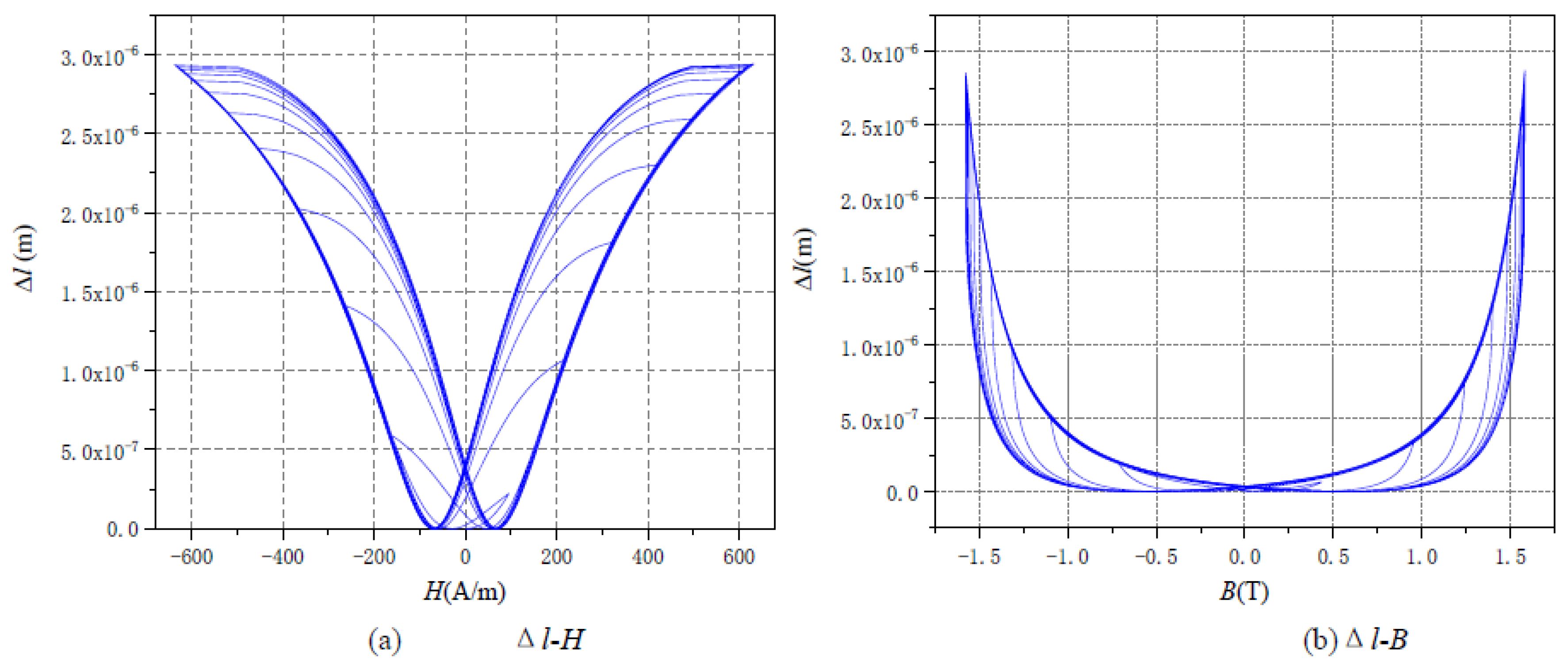
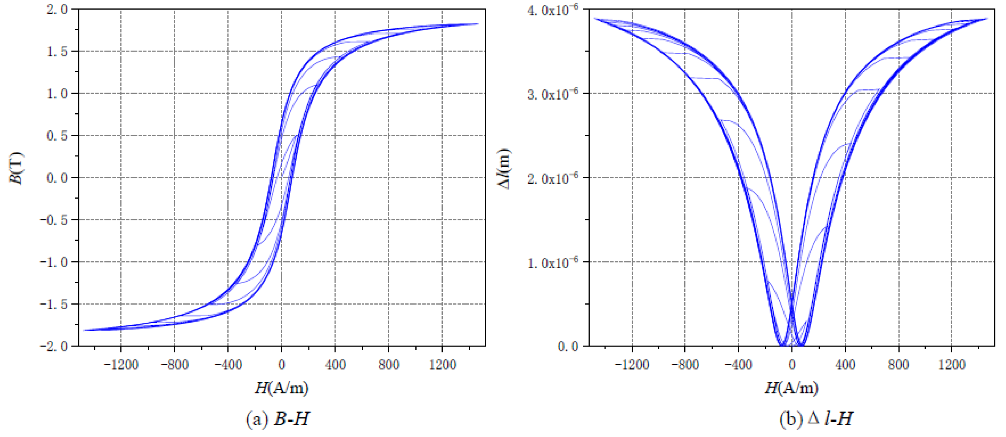
When there was no DC bias, the curves of the relationship between the magnetostrictive deformation and the magnetic field showed butterfly shapes, indicating that the magnetostriction had hysteresis characteristics relative to the magnetic field.

(2)

The left and right wings of the deformation curves were symmetrical about the magnetic field. When the peak value of the AC voltage increased to a certain extent, the deformation curve bent, which shows that the magnetostriction also had saturation characteristics.

(3)

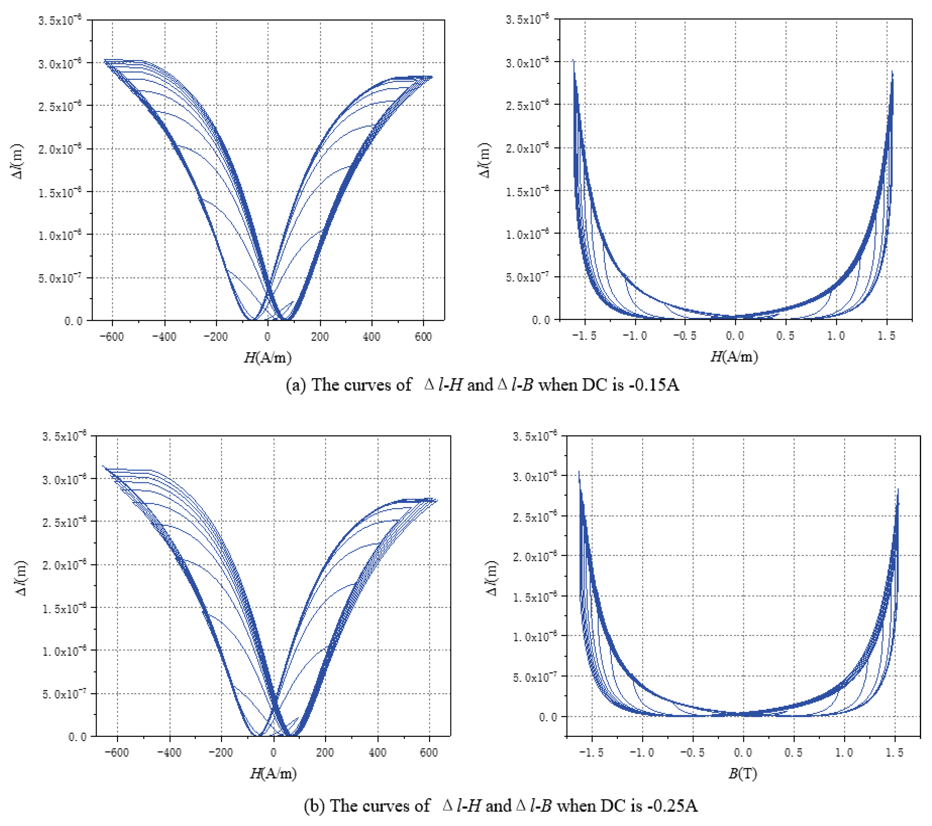
The left and right wings of the magnetostrictive deformation curves lost symmetry; that is, one became larger and the other faded under DC bias. Compared with the case without DC bias, the differences between the maximum values of the two wings increased, and the sensitivity of the magnetostrictive deformation to the change in the AC signal enhanced under the influence of the DC bias.

(4)

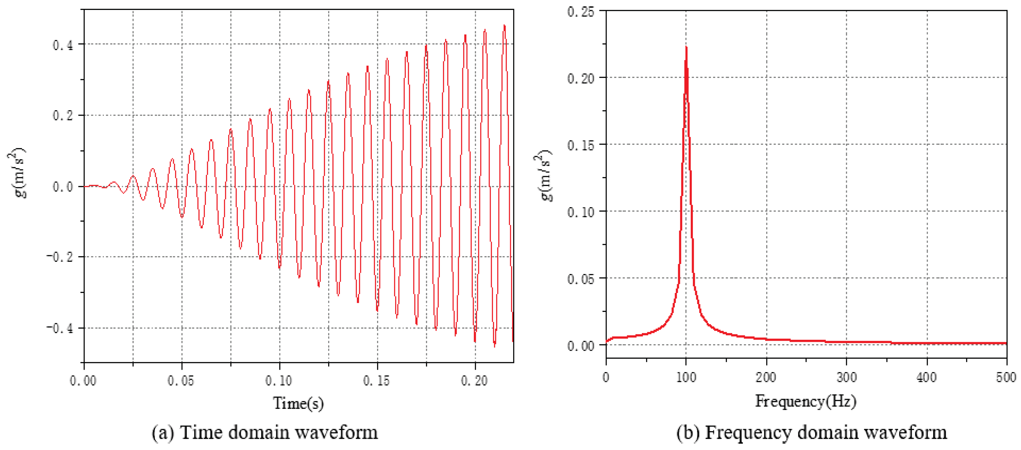
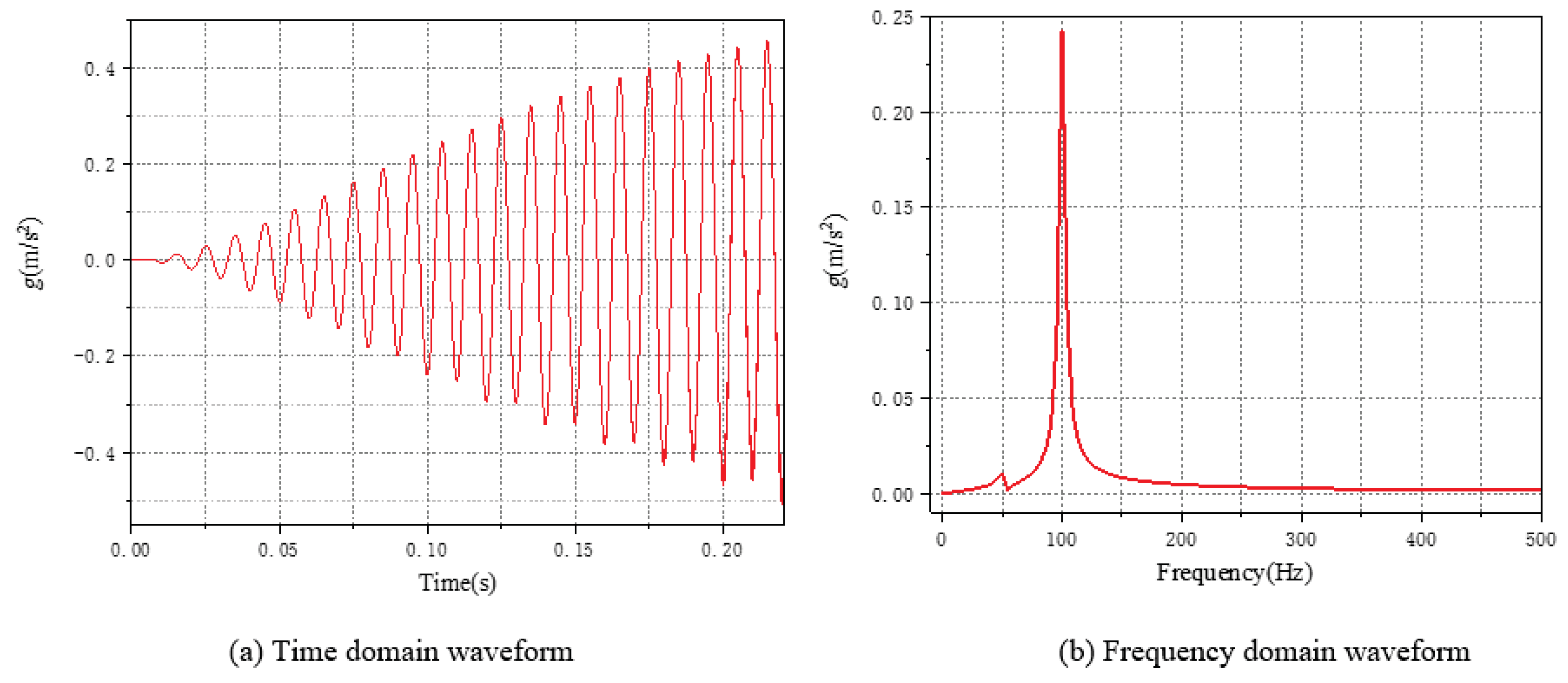
The amplitude of the vibration acceleration was concentrated at 100 Hz; that is, compared with the applied voltage frequency, the frequency of the vibration doubled. When there was DC bias, the amplitude at 100 Hz increased significantly. At the same time, a small wave peak appeared at 50 Hz.

(5)

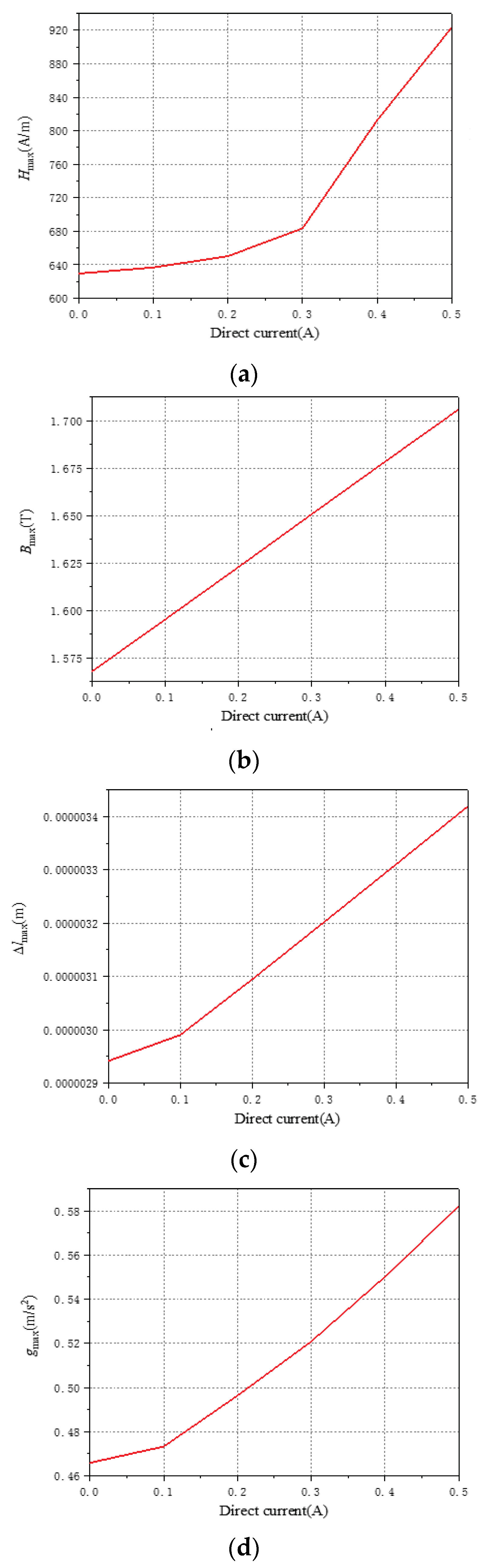
The magnetic field, magnetostrictive deformation, and vibration acceleration basically changed linearly with the increase in the DC. There were inflection points at 0.3 A DC for the magnetic field intensity curve and at 0.1 A DC for the magnetostrictive deformation and vibration acceleration curves. After these inflection points, the curves become obviously steeper, which suggests that the effect of the DC on them became significantly stronger.

(6)

The main research object of this article was single-phase transformers. The three-phase transformer group can be regarded as three single-phase transformers, so the uniform transmission line model (TLM) based on J–A theory can be used to study the electromagnetic and vibration characteristics of three-phase transformers.

(7)

Transformer DC bias affects the magnetostrictive properties of the core, which increases transformer vibration and noise. This paper provides theoretical ideas for finding measures to suppress DC bias, as well as transformer noise reduction measures.

References

1. Pan, C.; Wang, C.; Su, H. Excitation Current and Vibration Characteristics of DC Biased Transformer. CSEE J. Power Energy Syst. 2021, 7, 604–613. [Google Scholar]
2. Wang, Y.; Gao, C.; Li, L. Study for Influence of Harmonic Magnetic Fields on Vibration Properties of Core of Anode Saturable Reactor in HVDC Converter Valve System. IEEE Access 2021, 9, 24050–24059. [Google Scholar] [CrossRef]
3. Liu, C.; Li, X.; Li, X. Simulating the vibration increase of the transformer iron core due to the DC bias. Int. J. Appl. Electromagn. Mech. 2017, 55, 423–433. [Google Scholar] [CrossRef]
4. Li, Y.; Zhu, J.; Zhu, L. A Dynamic Magnetostriction Model of Grain-Oriented Sheet Steels Based on Becker-Döring Crystal Magnetization Model and Jiles-Atherton Theory of Magnetic Hysteresis. IEEE Trans. Magn. 2020, 56, 7511405. [Google Scholar] [CrossRef]
5. Lu, W.; Lei, G. Vibration and noise of oil-immersed auto-transformers. J. Vib. Shock. 2019, 38, 273–280. [Google Scholar]
6. Somkun, S.; Moses, A.J.; Anderson, P.I. Measurement and modeling of 2-D magnetostriction of nonoriented electrical steel. IEEE Trans. Magn. 2012, 48, 711–714. [Google Scholar] [CrossRef]
7. Zhang, Y.; Wang, J.; Bai, B. Influence Analysis of DC Biased Magnetic Field on Magnetostrictive Characteristics of Silicon Steel Sheet. Proc. CSEE 2016, 36, 4299–4307. [Google Scholar]
8. Wang, J.; Bai, B.; Liu, H. Research on Vibration and Noise of Transformers under DC Bias. Trans. China Electrotech. Soc. 2015, 30, 56–61. [Google Scholar]
9. Han, F.; Li, Y.; Jing, Y. Numerical Calculation of Magnetostrictive Force for EHV Transformer Core Silicon Steel. High Volt. Eng. 2017, 43, 980–986. [Google Scholar]
10. He, Q.; Nie, J.; Zhang, S. Study of Transformer Core Vibration and Noise Generation Mechanism Induced by Magnetostriction of Grain-Oriented Silicon Steel Sheet. Shock. Vib. 2021, 2021, 8850780. [Google Scholar]
11. Ben, T.; Chen, F.; Chen, L. An Improved Magnetostrictive Model of Non-oriented Electrical Steel Sheet Considering Force-magnetic Coupling Effect. Proc. CSEE 2021, 41, 5261–5370. [Google Scholar]
12. Zhang, L.; Wang, G.; Dong, P. Study on the vibration of grain-oriented transformer core based on the intrinsic characteristics. Proc. CSEE 2016, 36, 3990–4001. [Google Scholar]
13. Hu, J.; Liu, D.; Liao, Q.; Yan, Y.; Liang, S. Analysis of Transformer Electromagnetic Vibration Noise Based on Finite Element Method. J. Electr. Eng. Technol. 2016, 31, 81–88. [Google Scholar]
14. Li, B.; Wang, Z.; Liu, H.; Li, H.; Liu, J. Experimental study of vibration noise of 500kV single-phase transformer under DC bias magnetism. J. Electr. Eng. Technol. 2021, 36, 2801–2811. [Google Scholar]
15. Lobry, J.; Trecat, J.; Broche, C. The transmission line modeling (TLM) method as a new iterative technique in nonlinear 2-D magnetostatics. IEEE Trans. Magn. 1996, 32, 559–566. [Google Scholar] [CrossRef]
16. Thomas, D.W.P.; John, P.; Okan, O. Time-Domain Simulation of Nonlinear Transformers Displaying Hysteresis. IEEE Trans. Magn. 2006, 42, 1820–1827. [Google Scholar] [CrossRef]
17. Im, C.H.; Kim, H.K.; Le, C.H. Analysis of the three-phase transformer considering the nonlinear and anisotropic properties using the transmission line modeling method and FEM. IEEE Trans. Magn. 2001, 37, 3490–3493. [Google Scholar]
18. Jiles, D.C.; Atherton, D.L. Theory of Ferromagnetic Hysteresis. J. Magn. Magn. Mater. 1986, 61, 48–60. [Google Scholar] [CrossRef]
19. Jiles, D.C.; Thoelke, J.B.; Devine, M.K. Numerical Determination of Hysteresis Parameters for the Modeling of Magnetic Properties Using the Theory of Ferromagnetic Hysteresis. IEEE Trans. Magn. 1992, 28, 7–35. [Google Scholar] [CrossRef]
20. Liu, Y.; Luo, X.; Zhu, H. Modeling plastic deformation effect on the hysteresis loops of ferromagnetic materials based on modified Jiles-Atherton model. Acta Phys. Sin. 2017, 66, 1–11. [Google Scholar]
21. Luo, X.; Zhu, H.; Ding, Y. A modified model of magneto-mechanical effect on magnetization in ferromagnetic materials. Acta Phys. Sin. 2019, 68, 187501. [Google Scholar] [CrossRef]
Figure 1. The single-phase transformer circuit model.
Energies 16 04457 g001
Figure 2. The calculation process.
Energies 16 04457 g002
Figure 3. The single-phase transformer TLM circuit: (a) transmission line model equivalent circuit of the primary winding; (b) transmission line model equivalent circuit of the secondary winding; (c) equivalent circuit of the transmission line model with additional windings.
Energies 16 04457 g003
Figure 4. The curves of ∆l−H and ∆l−B without DC bias.
Energies 16 04457 g004
Figure 5. The single—phase transformer TLM circuit.
Energies 16 04457 g005
Figure 6. The waveform of the vibration acceleration without DC bias.
Energies 16 04457 g006
Figure 7. Curve of the relationship between the magnetostrictive deformation and the magnetic field with DC bias.
Energies 16 04457 g007
Figure 8. The waveform of the vibration acceleration when the DC is −0.25 A.
Energies 16 04457 g008
Figure 9. The variation curves of the transformer’s electromagnetic characteristics with DC: (a) variation curve of the magnetic field’s strength with DC; (b) variation curve of the magnetic flux density with DC; (c) variation curve of the magnetostrictive deformation with DC; (d) variation curve of the vibration acceleration with DC.
Energies 16 04457 g009